Communication

Distinguishing Buildings from Vegetation in an Urban-Chaparral Mosaic Landscape with LiDAR-Informed Discriminant Analysis

by
Thomas J. Yamashita
1,*,
David B. Wester
1,
Michael E. Tewes
1,
John H. Young, Jr.
2 and
Jason V. Lombardi
1,†
1
Caesar Kleberg Wildlife Research Institute, Texas A&M University—Kingsville, Kingsville, TX 78363, USA
2
Environmental Affairs Division, Texas Department of Transportation, Austin, TX 78701, USA
*
Author to whom correspondence should be addressed.
Current address: Wildlife Health Laboratory, California Department of Fish & Wildlife, Rancho Cordova, CA 95670, USA.
Remote Sens. 2023, 15(6), 1703; https://doi.org/10.3390/rs15061703
Submission received: 1 February 2023 / Revised: 14 March 2023 / Accepted: 20 March 2023 / Published: 22 March 2023

Abstract

:
Identification of buildings from remotely sensed imagery in urban and suburban areas is a challenging task. Light detection and Ranging (LiDAR) provides an opportunity to accurately identify buildings by identification of planar surfaces. Dense vegetation can limit the number of light particles that reach the ground, potentially creating false planar surfaces within a vegetation stand. We present an application of discriminant analysis (a commonly used statistical tool in decision theory) to classify polygons (derived from LiDAR) as either buildings or a non-building planar surfaces. We conducted our analysis in southern Texas where thornscrub vegetation often prevents a LiDAR beam from fully penetrating the vegetation canopy in and around residential areas. Using discriminant analysis, we grouped potential building polygons into building and non-building classes using the point densities of ground, unclassified, and building points. Our technique was 95% accurate at distinguishing buildings from non-buildings. Therefore, we recommend its use in any locale where distinguishing buildings from surrounding vegetation may be affected by the proximity of dense vegetation to buildings.

1. Introduction

Image classification is essential to the analysis of spatial patterns and is widely used in many disciplines, including landscape ecology, forestry, geography, hydrology, environmental engineering, and others [1]. However, decisions and management actions that are based on these classified images are only useful when the classification itself is accurate [2]. Therefore, it is important to accurately classify the image. In urban and suburban areas, buildings often are difficult to identify using traditional classification techniques such as supervised and unsupervised classification because of the wide variety of roof colors and shapes [3,4]. In addition, vegetation may overshadow buildings, which could vastly underestimate urban landcover. Several machine-learning-based techniques have been developed to help identify complex features such as buildings including image segmentation, object-oriented classification, and convolutional neural networks; however, these methods are still limited by obscuration by shadows or trees.
Light detection and ranging (LiDAR) provides an alternative method for distinguishing buildings from surrounding vegetation. LiDAR works by shooting a laser beam at the ground, usually from an aerial or terrestrial platform, then measuring the height and position of each particle that returns to the sensor. The resulting point cloud is used to create a three-dimensional model of the landscape [5]. This makes it an ideal tool for identifying buildings because roofs tend to be planar surfaces that can be readily distinguished from the more complex vegetation surfaces. Although several highly accurate techniques exist to identify buildings from a LiDAR point cloud, including the RANSAC algorithm [6,7], convolutional neural networks (CNN) [8], point cloud segmentation [9], density-based clustering [10], and a combination of CNN and clustering [11], these methods often rely on complex algorithms that are rarely made available to fellow researchers. An alternative to algorithm-based or deep learning approaches is to use freely and commercially available software such as LAStools, TerraSolid, and LP360 [12,13,14]. However, the building classifiers in these software packages, if they exist, are often poor at distinguishing buildings from complex vegetation, especially shrubs with dense foliage and complex internal branch structure [9]. Software-based approaches typically use last return points to identify flat planes of a user-specified size and angle [14]. However, this technique only works when there are no or very few last return points above the ground within surrounding vegetation. In forests and woodlands, there tends to be more space between branches and leaves, allowing the laser to penetrate the canopy. However, in shrublands with dense woody vegetation that can grow to >5 m, branches and leaves often prevent the laser from reaching the ground. Because of the high density of last return points within this type of vegetation, often at the same height as buildings, planar point algorithms can mistake these areas as being buildings. Therefore, a method that is simple for most users is needed to distinguish these false buildings from true buildings.
Discriminant analysis, originally developed by Fisher in 1936 [15], is a commonly used statistical tool with applications that range from inference (i.e., drawing inferences about the relationship between a categorical variable(s) that define(s) group membership and a set of interrelated continuous variables associated with members of each group) to decision theory (where the goal is “outright assignment” of an object to a group based upon the associated variables) ([16], p. 2). Most applications of discriminant analysis fall between these two extremes and involve “a prediction or tentative allocation of an unclassified entity” ([16], p. 2) into one of several groups. In this paper, we use discriminant analysis to assign an observation of unknown origin (in this case, a polygon derived from LiDAR) to one of two distinct groups—either a building or a non-building planar surface—based on how observed values of two or more variables associated with that observation compares to group means for those same variables [11]. Building roofs are impervious surfaces that the LiDAR beam cannot penetrate, so there are often few ground points. Therefore, most of the non-ground points are classified as buildings by the planar point filter within a polygon identified as a building. However, in vegetation polygons, there is often more variation in the classified point cloud, including large numbers of ground and unclassified points and fewer points classified as buildings. Therefore, we can use the proportions of the points classified as ground, building, and other points to distinguish between buildings and vegetation in shrublands.
In this note, we describe an extension to software-based building-classification that increases accuracy and feasibility in areas with complex vegetation. The purpose of our method is to provide a fast and easy-to-use addition to software-based building classification that improves accuracy when complex vegetation would otherwise prevent the use of software-based building classification. We first describe how we identified potential building polygons, then describe how point statistics and discriminant analysis can be used to distinguish building points from vegetation.

2. Materials and Methods

2.1. Study Area

We conducted this study in eastern Cameron County, Texas, USA, in a heterogeneous landscape of low to high-density urban areas, thornscrub, and coastal prairie [17]. The study area consisted of a 3 km buffer around State Highway 100 to the south, Farm-to-Market (FM) 1847 to the west, and FM 106 to the north and east (Figure 1). The towns of Bayview, Laguna Vista, Los Fresnos, and Rio Hondo are located within the study area. Laguna Atascosa National Wildlife Refuge (LANWR) and privately owned agriculture, wind farm, and ranchland make up a large proportion of the remaining study area. This part of Cameron County has a large amount of thornscrub vegetation, which is a dense, shrubby vegetation community that typically reaches 3–5 m tall [18]. The dense internal structure of thornscrub often prevents a LiDAR pulse from reaching the ground, causing last-return points to occur at the same height (~3 m), as a one-story building.

2.2. LiDAR Point Cloud

We obtained a LiDAR point cloud collected in 2018 by the United States Geological Survey using an airborne LiDAR system from the Texas Natural Resources Information System in September 2020 [19]. The LiDAR dataset covered the entire study area and had a nominal point spacing (NPS) of 0.7 m. Ground points, low noise, high noise, water, and bridge decks had been classified before the public release of the data according to specifications from the U.S. Geologic Survey [20]. The remaining points were left as unclassified points.

2.3. Building Classification

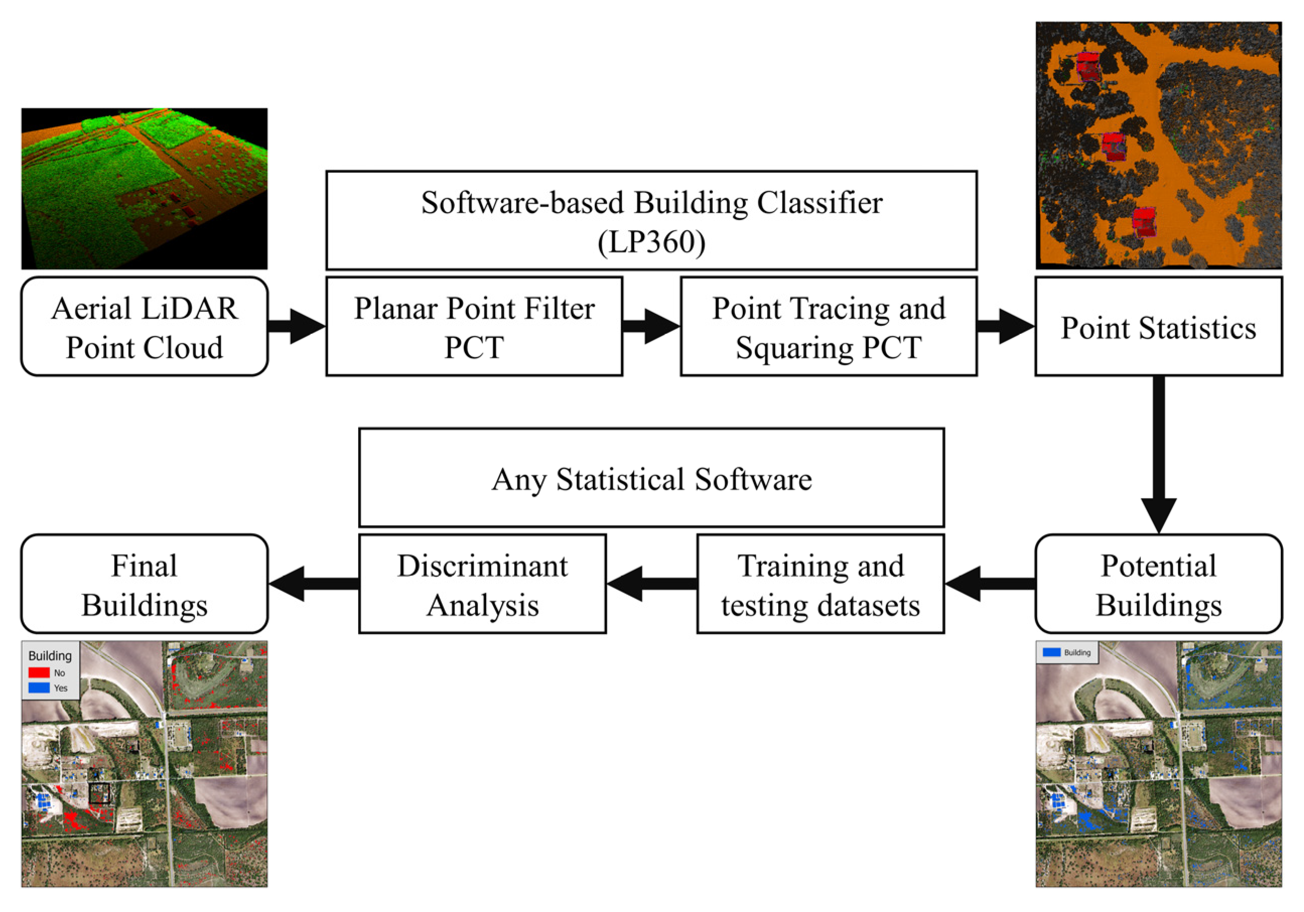
We used the planar point filter point cloud task (PCT) and planar tracing and squaring PCT in the program LP360 (GeoCue Group Inc., Madison, AL, USA) to perform our initial, software-based building classification (Figure 2). The settings of these PCTs can have major consequences for the resulting classification, so we optimized these settings by focusing on a small testing area near the headquarters of LANWR, an area made up of thornscrub with some buildings interspersed in the area. After settings were chosen for this area, five additional sites were selected to represent the variation in urban intensity and vegetation density within the study area to aid in optimization for the entire study area (see Appendix A for a full description of settings and the optimization strategy used). These settings were then applied to the full study area.
Using the point cloud data, we identified LiDAR returns that may represent buildings with the planar point filter PCT, then used the planar tracing and squaring PCT to draw polygons of potential buildings. During the classification of the full study area, some returns that were classified as buildings by the planar point filter PCT were not included as a building during the planar tracing and squaring PCT. We reclassified these returns as their own class to distinguish them from buildings and unclassified points, calling them non-buildings.
We calculated point statistics for each building polygon produced by the planar tracing and squaring PCT using the planar statistics PCT. Using all available returns, we calculated the number of returns of ground, unclassified, building, low noise, water, rail, bridge deck, high noise, and non-buildings. These classes represented all the possible points within each polygon. Unclassified returns were those returns above the ground level and were not classified as buildings or non-buildings, and so likely represented vegetation. We calculated proportions of returns for each class to standardize return counts by polygon area.

2.4. Discriminant Analysis

To formulate discriminant analysis for this setting, we define the following: (1) units to be classified are polygons that are derived from LiDAR (see above); (2) the populations to which polygons are classified are (a) buildings, or (b) non-building planar surfaces; (3) each polygon has associated with it the proportion of the following “return types” (see above): (a) ground, (b) unclassified, and (c) building. Thus, each observation (polygon) in the dataset is described by a p-dimensional vector of random variables, where p = 3 point types. The goal achieved by discriminant analysis is the assignment of each polygon to one of two populations based on its Mahalanobis’ distance to population centroids.
We considered all available polygons created by the point tracing and squaring PCT as the population of potential buildings within the study area. We sampled 500 polygons from this population to create a training dataset for discriminant analysis and an additional 500 polygons to serve as a testing dataset to validate the training data and assess accuracy. Our sample size exceeds recommendations based on theoretical considerations [21] as well as common recommendations in the applied literature (e.g., [22,23,24]). We manually classified each training and testing sample into building or not building using National Agriculture Imagery Program aerial images from 2016 (1 m resolution) and 2020 (0.6 m resolution) [25]. The 2018 imagery was not available/redacted for much of the southern part of the study area, where most buildings were located, so we did not use this imagery.
We calculated the proportion of each type of point within each sampled polygon. We tested for multivariate normality using graphical methods and the Henze-Zirkler’s and Royston’s tests available in the MVN package in R [26,27] and for equality of covariance matrices using Box’s M test in the MVTests package in R [28,29]. We transformed the data using the arcsine transformation to improve multivariate normality of the data. The ground, unclassified, and building classes made up 4.68–100% of the points in each polygon (mean 98.49%, median 100%) so we only used these three classes for analysis. The small number of polygons with low proportions of these three classes typically had high proportions of water. To confirm differences between groups, we ran a MANOVA on the training dataset and tested significance using the Wilks Lambda and Roy’s Maximum Root tests [30]. We performed a quadratic discriminant analysis with unequal prior probabilities to predict the classification of each polygon using the “qda” function in the MASS package in R [31]. We assumed that the sampled proportions of each class (from the training and testing datasets) reasonably estimated the population proportions of those classes, so we used the proportion of each class in the training dataset as the prior probabilities for the two classes.
We used the means and covariance matrices of the training dataset to predict the classification of the testing dataset to assess the accuracy of the analysis before applying the prediction to the entire dataset [30]. After we were satisfied with the accuracy, we applied the analysis to the entire dataset. We performed a separate accuracy assessment on the full dataset using a confusion matrix by manually classifying 500 polygons classified as buildings and 500 classified as non-buildings [32].

3. Results

After running the software-based building classification, we identified 49,553 polygons as potential buildings. The final settings are summarized in Table 1. In our training dataset, 107 polygons were buildings, and 393 polygons were vegetation and in our testing dataset, 109 polygons were buildings, and 391 polygons were vegetation. After transformation, the training dataset was not normally distributed for buildings (Henze-Zirkler’s HZ = 5.31, p < 0.0001, Royston H = 13.90, p = 0.0007) or for non-buildings (Henze-Zirkler’s HZ = 20.32, p < 0.0001, Royston H = 51.78, p < 0.0001); however, graphical measures showed approximate normality for both groups. Additionally, it is well known (e.g., [33], p. 454) that with large sample sizes, goodness of fit tests usually result in rejection. Box’s M test showed a statistically significant difference in the variance–covariance matrices for the building and non-building groups (Χ2 = 154.79, p < 0.0001), allowing use of quadratic discriminant analysis instead of nonparametric methods [30]. The average proportions of points for building polygons was different from non-building polygons (pseudo-F = 413.7 for Wilks lambda and Roy’s maximum root, p < 0.0001 for both) with building proportion being greater in building polygons and ground and unclassified proportions being greater in non-building polygons (Table 2).
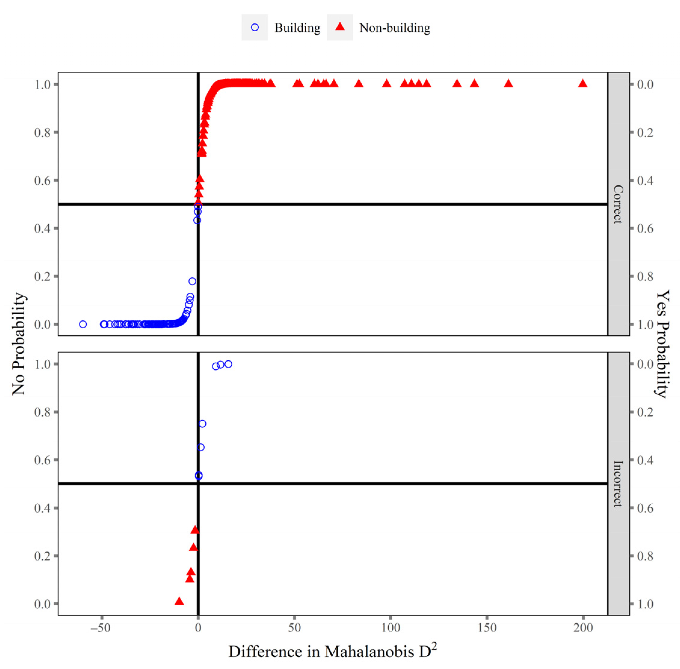
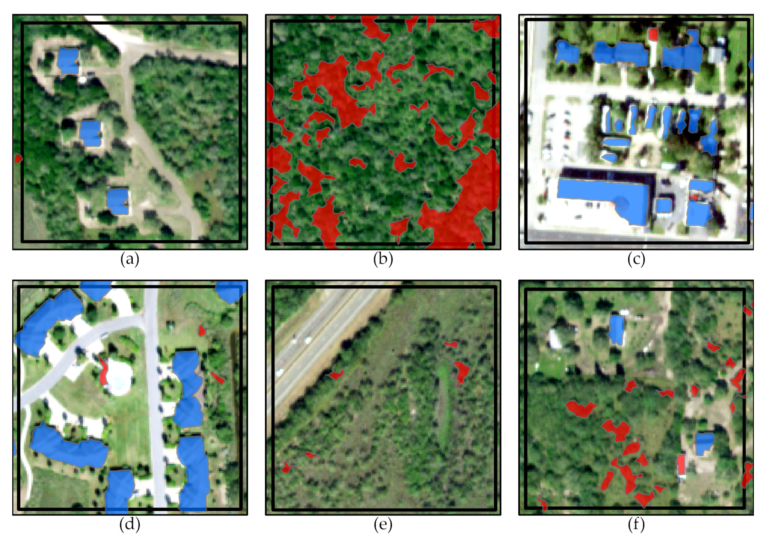
When we used our training dataset to predict the group membership of the testing dataset based on the three classes, the model was 97.6% accurate at identifying buildings (Figure 3). Therefore, we applied this model to the full dataset (Figure 4). The additional accuracy assessment on the 1000 building and non-building polygons was 95.4% accurate.

4. Discussion

Using a software-based building classification and discriminant analysis, we were able to use LiDAR to identify buildings accurately 95% of the time when using the proportions of returns classified as ground, unclassified, and buildings. Our analysis effectively distinguished buildings from vegetation and can therefore be used to support image classification and as a stand-alone product in ecology, urban planning and design, environmental engineering, conservation biology, and others. Importantly, our method is user-friendly, highly accurate, and does not require the development of complex algorithms or a strong understanding of machine learning methods.
Identifying buildings using LiDAR allows researchers to distinguish urban areas more effectively and precisely from other landcover types. Several different methods have been developed previously to identify buildings from LiDAR data, including by combining LiDAR with imagery segmentation (accuracy: 90%; [4]), using fitted surfaces and morphological profiles (accuracy: >95%; [34]), and software-based approaches, similar to those used in this study (accuracy not assessed; [14]). However, these studies were conducted in city environments where vegetation was sparse or could be clearly defined. In suburban and rural areas where the vegetation matrix is made up primarily of shrubs or dense tree stands, it becomes more difficult to distinguish buildings from background vegetation. Algorithm-based approaches using the RANSAC algorithm (accuracy: 97%; [6]), deep learning CNN (accuracy: 93%; [8]), cluster-based approaches (accuracy: 95%; [11]), and segmentation of the point cloud (accuracy: 95%; [9]) have been shown to be effective at distinguishing buildings from complex vegetation; however, these are often complex processes that are difficult to accomplish without extensive knowledge of programming that many applied researchers do not have. Our method of expanding simple software-based approaches with the addition of discriminant analysis can accurately identify buildings in heterogeneous, complex landscapes. Additionally, using standard LiDAR software (LP360) and discriminant analysis (which can be run in many standard statistical software packages, including R, SAS, and SPSS), we provide a user-friendly method for performing building identification.
Software-based approaches often require fine-tuned adjustment of various parameters to ensure that one maximizes the capture of buildings while minimizing capture of vegetation areas [35]; however, this may not be important using our technique because the discriminant analysis can do this for us. Although we recommend that some effort be made to adjust planar identification settings, we argue that it is more important to ensure capture of all buildings rather than balancing building capture with the exclusion of vegetation areas.
As LiDAR data become more available through expanding coverage of aerial LiDAR and the development of satellite LiDAR systems such as the ICESat-2 satellite, the use of LiDAR data is expanding to more urban areas where identification of buildings is becoming increasingly important. Our method can be used by applied scientists including remote sensors, ecologists, and urban planners alike to model landcover change, assess urban growth and development, or examine the relationship between animal space use and buildings at fine spatial scales. This method can be applied anywhere where dense vegetation may affect the identification of planar surfaces, including Tamaulipan thornscrub of southern Texas and northern México (this study), the chaparral of southern California [36], the Miombo woodlands of central and southern Africa [37], or tropical forests with dense understories in Asia and South America [38].
Although our method is highly accurate, it may not be appropriate in all cases. Using software-based building classification requires a large amount of computing power. Our analysis of 210 1.5 km × 1.5 km LiDAR tiles (~472.5 km2) took approximately 475 computing hours (89 h for the planar point filter, 36 h for the point tracing and squaring, and 350 h for the planar statistics PCTs) using a laptop computer with an Intel I7-6820HQ processor, 32 GB of RAM, and an Nvidia Quadro M3000M graphics card. The discriminant analysis, however, ran in seconds on the same machine. To save on processing time, we would not recommend this technique if one were working in rural areas with low numbers of buildings. In the case of a few buildings (under 1000), we would recommend digitizing each manually and verifying buildings using a classified image. However, if one uses software-based building classification tools or if they are not comfortable developing a machine learning model, then we would recommend using discriminant analysis to improve the building identification.
Identification of buildings is a crucial step in studies on the urban environment and human impacts on the environment. We have demonstrated the usefulness and simplicity of discriminant analysis in improving the identification of buildings from a LiDAR point cloud. This technique has broad applications in many disciplines and locales, and we recommend its use anywhere where distinguishing buildings from surrounding vegetation may be challenging.

Author Contributions

Conceptualization, T.J.Y., D.B.W. and J.V.L.; methodology, T.J.Y., D.B.W. and J.V.L.; validation, T.J.Y.; formal analysis, T.J.Y. and D.B.W.; investigation, T.J.Y.; data curation, T.J.Y.; writing—original draft preparation, T.J.Y.; writing—review and editing, T.J.Y., D.B.W., J.V.L., M.E.T. and J.H.Y.J.; visualization, J.V.L.; supervision, J.V.L.; project administration, J.V.L., M.E.T. and J.H.Y.J.; funding acquisition, J.V.L., J.H.Y.J. and M.E.T. All authors have read and agreed to the published version of the manuscript.

Funding

This research was funded by the Texas Department of Transportation.

Data Availability Statement

LiDAR point cloud data and NAIP imagery were freely downloaded from the Texas Natural Resources Information System: https://data.tnris.org, accessed on 1 February 2021. A shapefile of potential building polygons counts of points for each polygon, the training dataset, testing dataset, accuracy dataset, and associated R code are available on GitHub at https://github.com/tomyamashita/DistinguishingBuildingsFromVeg.

Acknowledgments

We thank the Texas Department of Transportation for financial support for TJ Yamashita and JV Lombardi. We thank J Baumgardt and H Perotto-Baldivieso for reviewing earlier versions of the manuscript. This manuscript is #22-124 of the Caesar Kleberg Wildlife Research Institute.

Conflicts of Interest

The authors declare no conflict of interest.

Appendix A

This Appendix provides a list of steps to capture buildings from LiDAR data and make a distinction between true buildings and non-buildings in semi-arid chaparral woody habitats. This appendix also provides sample code in both R and SAS for using quadratic discriminant analysis to predict the group classification of new observations.

Appendix A.1. Part 1: Processing LiDAR Data

Before we can distinguish buildings from non-buildings, we have to create the polygons and calculate point densities. This was done in the program LP360 (GeoCue Group Inc., Madison, AL, USA). While we provide the list of settings we used for our study area, these may differ in different regions and habitats. We recommend optimizing settings that maximize capture of all buildings for your particular study area. Steps 1–3 apply to this optimization process.
Step 1: Determine optimal settings for capturing all buildings in the study area using a small focal area for the Planar Point Filter Point Cloud Task (PCT).
Step 2: Determine optimal settings for capturing all buildings in the study area using a small focal area for the Point Tracing and Squaring PCT.
Step 3: Test and adjust these settings as necessary on at least one other focal site to ensure that buildings are being captured in those locations as well.
Step 4: Apply the Planar Point Filter PCT on your full study area.
Step 5: Apply the Point Tracing and Squaring PCT on the full study area.
Step 6: Calculate point counts within each non-squared polygon using the Planar Statistics PCT of all available points, not just last return points.
We used the planar point filter point cloud task (PCT), planar tracing and squaring PCT, and planar statistics PCT in the program LP360 (GeoCue Group Inc., Madison, AL, USA) to identify potential buildings. LiDAR does not penetrate buildings, so we only used last-return points for our analyses. To optimize the settings for the PCTs, we focused on a small testing area near the headquarters of LANWR, an area made up of thornscrub with some buildings interspersed within the area. After settings were optimized for this location, we further refined them at five additional sites, subjectively chosen to have different properties: thornscrub on LANWR with no buildings, urban high-density site in Los Fresnos, urban low-density site in Laguna Vista, thornscrub-prairie habitat with no buildings, and a rural property near Los Fresnos with taller trees and some buildings.
For the planar point filter PCT, we were most interested in the minimum plane edge, plane fit, and N threshold settings. The minimum plane edge is the minimum square area for a plane, the plane fit is the amount that a point deviates from a surface perpendicular to the plane, and the N threshold is the maximum distance from a plane that a point can be to be considered part of the plane [35]. To start, we set the minimum plane edge to 2.1 m or three times the NPS of the LiDAR data, plane fit to 1.0 standard deviation, N threshold to 1.0 m, and the maximum growth window to 0 [35]. We also set the maximum height to an arbitrarily high height of 65 m. This height was above all buildings and trees, except for windmills (~60–90 m). Initially, we set our minimum height to 3 m, which was the approximate height of a one-story building. We set the minimum slope to 0° and maximum slope to 45°.
We first adjusted the minimum plane edge, increasing it incrementally by a maximum of 0.5 m until we achieved the peak number of planes identified [35]. We adjusted the plane fit incrementally down by 0.1 units until we reached the point where most of the planes created in trees were removed without removing any planes on buildings. Next, we adjusted the N threshold down incrementally by 0.1 m, then by smaller increments to further remove planes in trees without removing any planes in buildings. We set the maximum grow window to the default of 500 to ensure that we captured the full plane created by a building [35]. We also tested smaller (0) and larger (1000) grow windows using our finalized settings for plane fit and N threshold, but these did not improve the planar fit.
For the planar tracing and squaring PCT, we were interested in the grow window, trace window, and minimum area settings. We adjusted the grow window and trace window together because the trace window should be approximately two times the grow window [16]. We started with a grow window of 3.0, or approximately the recommended maximum for the grow window of four times the NPS, and a trace window of 6.0 [39]. Our starting minimum area was 100 m2. We then decreased the grow window incrementally by 0.5, then by smaller increments once we neared an optimal value. The trace window was adjusted proportionately with the grow window to ensure that it remained two times the grow window. Next, we tested different minimum areas. We decreased the minimum area incrementally by 25 m2 until we captured all buildings.
After the settings of the planar point filter PCT and planar tracing and squaring PCT were optimized for our primary testing area, we applied the PCTs to our secondary testing areas, further refining our settings to work across the different sites. Based on these tests, we further reduced our minimum height in the planar point filter PCT and minimum area in the planar tracing and squaring PCT to ensure that buildings were captured.
After settings were optimized for our test sites, we ran the planar point filter and the planar tracing and squaring PCTs on the entire study area.

Appendix A.2. Part 2: Discriminant Analysis

The next steps involve setting up and preparing data for discriminant analysis. It is important to sample enough observations from the available potential buildings to accurately assign group membership to an unknown polygon. While several forms of discriminant analysis exist (i.e., linear, quadratic, and nonparametric methods), we use quadratic discriminant analysis for our example. Quadratic discriminant analysis (QDA) differs from linear discriminant analysis (LDA) in that it does not assume that within variance–covariance matrices are homogeneous between groups; a standard reference is Johnson and Wichern ([40], Chapter 11).
Step 7: Sample the polygons from the full study area to use as a training dataset for the discriminant analysis. We recommend obtaining a minimum of 100 of each building and non-buildings.
Step 8: Sample an equal number of polygons as the training dataset to use as a testing dataset.
Step 9: Manually classify the training and testing datasets using a high-resolution image.
Step 10: Transform the proportions of ground, unclassified, and buildings using the arc-sine transformation. If prediction ability is low, other classes may be included to improve accuracy. We do not recommend using all available classes as this can cause issues with determinants equaling 0. In this case, the qda function in R often still runs, but it is incorrect.
Step 11: Run discriminant analysis in software of choice. Sample code for R and SAS are provided below. Full R code and data are available on GitHub at https://github.com/tomyamashita/DistinguishingBuildingsFromVeg.

Appendix A.3. Sample Code for Quadratic Discriminant Analysis in R and SAS
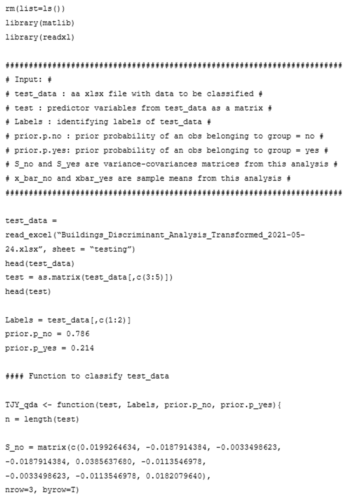
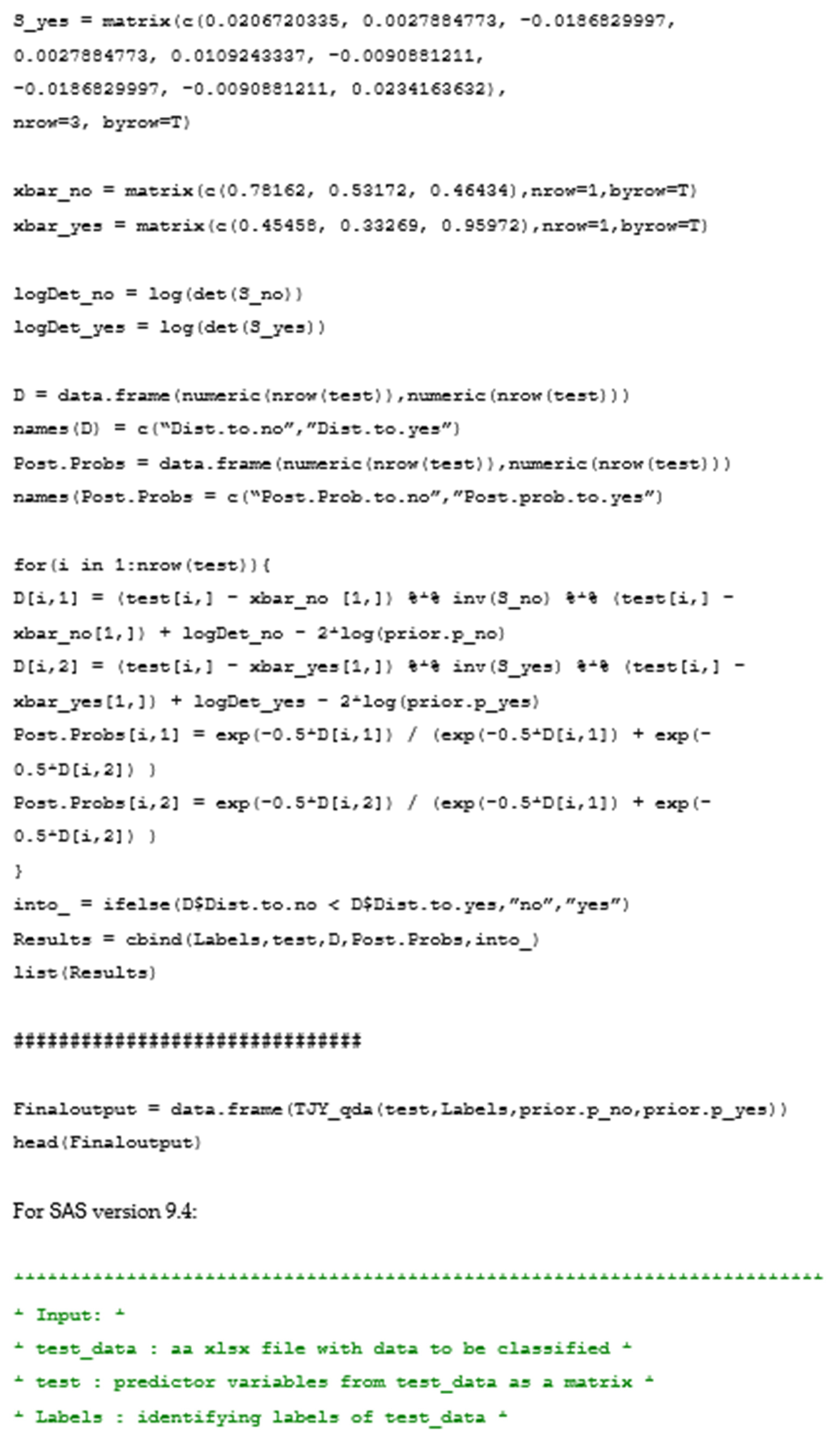
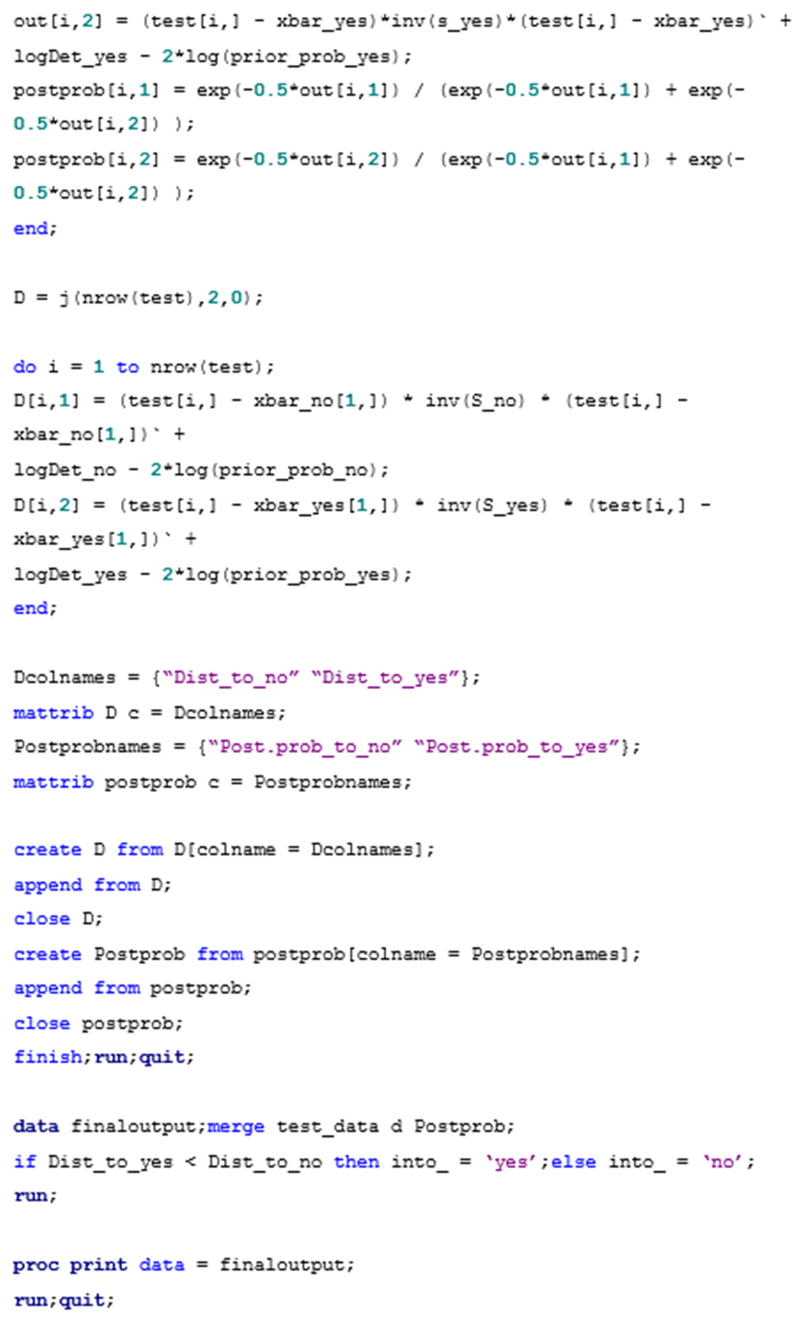
This section provides code for R and SAS that uses the estimated variance–covariance matrices and mean vectors (based on data from this analysis) to classify new observations. A dataset, named “test_data,” contains new observations to be classified. This dataset contains identifying information (“labels”) for n observations to be classified into two groups (building or non-building planar surfaces) based on three continuous variables that are point densities of vegetation, ground, and building, each of which are arc-sine transformed proportions. Prior probabilities are the proportions of a yes or a no in the training dataset from this analysis.
Note, while this example provides the variance–covariance matrices and mean vectors from our training dataset, these may not be applicable in all settings. While we provide the code here to use our training data to predict new observations, relative proportions of ground, unclassified, and building points could differ by the aerial LiDAR system used and study area, so we recommend that users develop situation-specific training and testing data using the code provided with the data.
For R Version 4.1.2: Remotesensing 15 01703 i001Remotesensing 15 01703 i002Remotesensing 15 01703 i003Remotesensing 15 01703 i004

References

  1. Kerle, N.; Janssen, L.L.F.; Huurneman, G.C. Principles of Remote Sensing, 3rd ed.; The International Institute for Geo-Information Science and Earth Observation (ITC): Enchede, The Netherlands, 2004. [Google Scholar]
  2. Abburu, S.; Golla, S.B. Satellite Image Classification Methods and Techniques: A Review. Int. J. Comput. Appl. 2015, 119, 20–25. [Google Scholar] [CrossRef]
  3. Kamusoko, C.; Aniya, M. Hybrid classification of Landsat data and GIS for land use/cover change analysis of the Bindura district, Zimbabwe. Int. J. Remote Sens. 2009, 30, 97–115. [Google Scholar] [CrossRef]
  4. Lee, D.H.; Lee, K.M.; Lee, S.U. Fusion of Lidar and Imagery for Reliable Building Extraction. Photogramm. Eng. Remote Sens. 2008, 74, 215–225. [Google Scholar] [CrossRef] [Green Version]
  5. Lefsky, M.A.; Cohen, W.B.; Parker, G.G.; Harding, D.J. Lidar Remote Sensing for Ecosystem Studies: Lidar, an emerging remote sensing technology that directly measures the three-dimensional distribution of plant canopies, can accurately estimate vegetation structural attributes and should be of particular interest to forest, landscape, and global ecologists. BioScience 2002, 52, 19–30. [Google Scholar] [CrossRef]
  6. Canaz Sevgen, S.; Karsli, F. An improved RANSAC algorithm for extracting roof planes from airborne lidar data. Photogramm. Rec. 2020, 35, 40–57. [Google Scholar] [CrossRef]
  7. Yi, Z.; Wang, H.; Duan, G.; Wang, Z. An Airborne LiDAR Building-Extraction Method Based on the Naive Bayes–RANSAC Method for Proportional Segmentation of Quantitative Features. J. Indian Soc. Remote Sens. 2021, 49, 393–404. [Google Scholar] [CrossRef]
  8. Maltezos, E.; Doulamis, A.; Doulamis, N.; Ioannidis, C. Building Extraction From LiDAR Data Applying Deep Convolutional Neural Networks. IEEE Geosci. Remote Sens. Lett. 2019, 16, 155–159. [Google Scholar] [CrossRef]
  9. Liu, M.; Shao, Y.; Li, R.; Wang, Y.; Sun, X.; Wang, J.; You, Y. Method for extraction of airborne LiDAR point cloud buildings based on segmentation. PLoS ONE 2020, 15, e0232778. [Google Scholar] [CrossRef]
  10. Huang, X.; Cao, R.; Cao, Y. A Density-Based Clustering Method for the Segmentation of Individual Buildings from Filtered Airborne LiDAR Point Clouds. J. Indian Soc. Remote Sens. 2019, 47, 907–921. [Google Scholar] [CrossRef]
  11. Gamal, A.; Wibisono, A.; Wicaksono, S.B.; Abyan, M.A.; Hamid, N.; Wisesa, H.A.; Jatmiko, W.; Ardhianto, R. Automatic LIDAR building segmentation based on DGCNN and euclidean clustering. J. Big Data 2020, 7, 102. [Google Scholar] [CrossRef]
  12. Zhao, C.; Jensen, J.; Weng, Q.; Currit, N.; Weaver, R. Application of airborne remote sensing data on mapping local climate zones: Cases of three metropolitan areas of Texas, U.S. Comput. Environ. Urban Syst. 2019, 74, 175–193. [Google Scholar] [CrossRef]
  13. McNamara, D.; Mell, W.; Maranghides, A. Object-based post-fire aerial image classification for building damage, destruction and defensive actions at the 2012 Colorado Waldo Canyon Fire. Int. J. Wildland Fire 2020, 29, 174–189. [Google Scholar] [CrossRef]
  14. Prerna, R.; Singh, C.K. Evaluation of LiDAR and image segmentation based classification techniques for automatic building footprint extraction for a segment of Atlantic County, New Jersey. Geocarto Int. 2016, 31, 694–713. [Google Scholar] [CrossRef]
  15. Fisher, R.A. The use of multiple measurements in taxonomic problems. Ann. Eugen. 1936, 7, 179–188. [Google Scholar] [CrossRef]
  16. McLachlan, G.J. Discriminant Analysis and Statistical Pattern Recognition; John Wiley & Sons, Inc.: Hoboken, NJ, USA, 1992. [Google Scholar]
  17. Elliott, L.F.; Diamond, D.D.; True, D.; Blodgett, C.F.; Pursell, D.; German, D.; Treuer-Kuehn, A. Ecological Mapping Systems of Texas: Summary Report; Texas Parks & Wildlife Department: Austin, TX, USA, 2014. [Google Scholar]
  18. Shindle, D.B.; Tewes, M.E. Woody Species Composition of Habitats used by Ocelots (Leopardus pardalis) in the Tamaulipan Biotic Province. Southwest. Nat. 1998, 43, 273–279. [Google Scholar]
  19. United States Geologic Survey. South Texas Lidar; United States Geologic Survey: Washington, DC, USA, 2018. [Google Scholar]
  20. Heidemann, H.K. Lidar Base Specification; 11-B4; U.S. Geological Survey: Reston, VA, USA, 2012; p. 114. [Google Scholar]
  21. Zavorka, S.; Perrett, J.J. Minimum Sample Size Considerations for Two-Group Linear and Quadratic Discriminant Analysis with Rare Populations. Commun. Stat. Simul. Comput. 2014, 43, 1726–1739. [Google Scholar] [CrossRef]
  22. NCSS Statistical Software. Discriminant Analysis. Available online: https://www.ncss.com/wp-content/themes/ncss/pdf/Procedures/NCSS/Discriminant_Analysis.pdf (accessed on 2 May 2022).
  23. Morrison, M.L. Influence of Sample Size on Discriminant Function Analysis of Habitat use by Birds. J. Field Ornithol. 1984, 55, 330–335. [Google Scholar]
  24. Williams, B.K.; Titus, K. Assessment of Sampling Stability in Ecological Applications of Discriminant Analysis. Ecology 1988, 69, 1275–1285. [Google Scholar] [CrossRef]
  25. United States Department of Agriculture. Texas NAIP Imagery; United States Department of Agriculture: Washington, DC, USA, 2016. [Google Scholar]
  26. Korkmaz, S.; Goksuluk, D.; Zararsiz, G. MVN: An R Package for Assessing Multivariate Normality. R J. 2014, 6, 151–162. [Google Scholar] [CrossRef] [Green Version]
  27. Mecklin, C.J.; Mundfrom, D.J. A Monte Carlo comparison of the Type I and Type II error rates of tests of multivariate normality. J. Stat. Comput. Simul. 2005, 75, 93–107. [Google Scholar] [CrossRef]
  28. Bulut, H. An R Package for multivariate hypothesis tests: MVTests. Technol. Appl. Sci. (NWSATAS) 2019, 14, 132–138. [Google Scholar] [CrossRef]
  29. Layard, M.W.J. A Monte Carlo Comparison of Tests for Equality of Covariance Matrices. Biometrika 1974, 61, 461–465. [Google Scholar] [CrossRef]
  30. Lachenbruch, P.A. Discriminant Analysis; Hafner Press: New York, NY, USA, 1975. [Google Scholar]
  31. Venables, W.N.; Ripley, B.D. Modern Applied Statistics with S; Springer: New York, NY, USA, 2002. [Google Scholar]
  32. Stehman, S.V. Selecting and interpreting measures of thematic classification accuracy. Remote Sens. Environ. 1997, 62, 77–89. [Google Scholar] [CrossRef]
  33. Conover, W.J. Practical Nonparametric Statistics, 3rd ed.; John Wiley & Sons, Inc.: New York, NY, USA, 1999. [Google Scholar]
  34. Mongus, D.; Lukač, N.; Žalik, B. Ground and building extraction from LiDAR data based on differential morphological profiles and locally fitted surfaces. ISPRS J. Photogramm. Remote Sens. 2014, 93, 145–156. [Google Scholar] [CrossRef]
  35. Graham, L. LP360 (Advanced): Planar Point Filter User Guide; QCoherent Software, LLC: Madison, AL, USA, 2013. [Google Scholar]
  36. Gray, J.T. Community Structure and Productivity in Ceanothus Chaparral and Coastal Sage Scrub of Southern California. Ecol. Monogr. 1982, 52, 415–434. [Google Scholar] [CrossRef]
  37. Frost, P. The ecology of miombo woodlands. In The Miombo in Transition: Woodlands and Welfare in Africa; Campbell, B., Ed.; Centre for International Forestry Research: Bogor, Indonesia, 1996; pp. 11–57. [Google Scholar]
  38. LaFrankie, J.V.; Ashton, P.S.; Chuyong, G.B.; Co, L.; Condit, R.; Davies, S.J.; Foster, R.; Hubbell, S.P.; Kenfack, D.; Lagunzad, D.; et al. Contrasting structure and composition of the understory in species-rich tropical rain forests. Ecology 2006, 87, 2298–2305. [Google Scholar] [CrossRef] [Green Version]
  39. Graham, L. Point Group Tracing and Squaring in LP360: A Heuristic Discussion of Parameter Settings; QCoherent Software, LLC: Madison, AL, USA, 2013. [Google Scholar]
  40. Johnson, R.A.; Wichern, D.W. Applied Multivariate Statistical Analysis, 6th ed.; Pearson Education, Inc.: Upper Saddle River, NJ, USA, 2007. [Google Scholar]
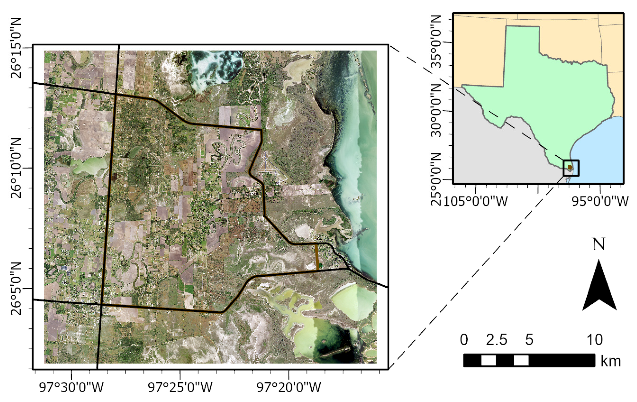
Figure 1. Study area showing State Highway 100, Farm-to-Market (FM) 1847, and FM 106 in Cameron County, Texas (black lines) and the LiDAR tiles used to identify buildings (brown polygon).
Remotesensing 15 01703 g001
Figure 2. Workflow for using a software-based building classifier and discriminant analysis to distinguish buildings from vegetation.
Remotesensing 15 01703 g002
Figure 3. Posterior probability of a polygon being correctly (top) or incorrectly (bottom) classified as a building or non-building in the testing dataset. The Mahalanobis D2 represents the distance in multivariate space from a set of ground, unclassified, and building proportions with unknown group assignment to the mean of known buildings (Yes) or known non-buildings (No). The difference is calculated as the distance to Yes—the distance to No. The vertical axes are the posterior probabilities of being classified as non-building (left) and building (right). Blue circles are buildings and red triangles are non-buildings.
Remotesensing 15 01703 g003
Figure 4. Building (blue) and non-building (red) as categorized by discriminant analysis after polygon creation by LP360 point cloud tasks at each of the test sites: (a) Laguna Atascosa National Wildlife Refuge (LANWR) Headquarters (original testing site), (b) LANWR thornscrub, (c) Los Fresnos, (d) Laguna Vista, (e) thornscrub-prairie habitat, (f) rural property near Los Fresnos.
Remotesensing 15 01703 g004
Table 1. List of settings and their values used for the Planar Point Filter and Point Tracing and Squaring point cloud tasks in LP360.
Point Cloud TaskSettingValue
Planar Point FilterInput PointsLast Returns Only
Minimum Height2 m
Maximum Height65 m
Minimum Slope
Maximum Slope45°
Minimum Plane Edge5.5 m
Plane Fit0.20 standard deviations
N Threshold0.025 m
Maximum Grow Window500 (unitless)
Point Tracing and SquaringGrow Window1.7 m
Trace Window3.4 m
Minimum Area25 m2
Table 2. Group mean proportion of LiDAR returns ± standard deviations for each arcsine transformed variable used in the training dataset for the discriminant analysis.
ClassificationBuildingNon-Building
Ground0.333 ± 0.1050.532 ± 0.196
Unclassified0.455 ± 0.1440.782 ± 0.141
Building0.960 ± 0.1530.464 ± 0.135
Disclaimer/Publisher’s Note: The statements, opinions and data contained in all publications are solely those of the individual author(s) and contributor(s) and not of MDPI and/or the editor(s). MDPI and/or the editor(s) disclaim responsibility for any injury to people or property resulting from any ideas, methods, instructions or products referred to in the content.