

Daily Sea Ice Concentration Product over Polar Regions Based on Brightness Temperature Data from the HY-2B SMR Sensor
 , ,
, ,
Abstract
1. Introduction
2. Data
2.1. HY-2B SMR Sensor
2.2. Published SIC datasets
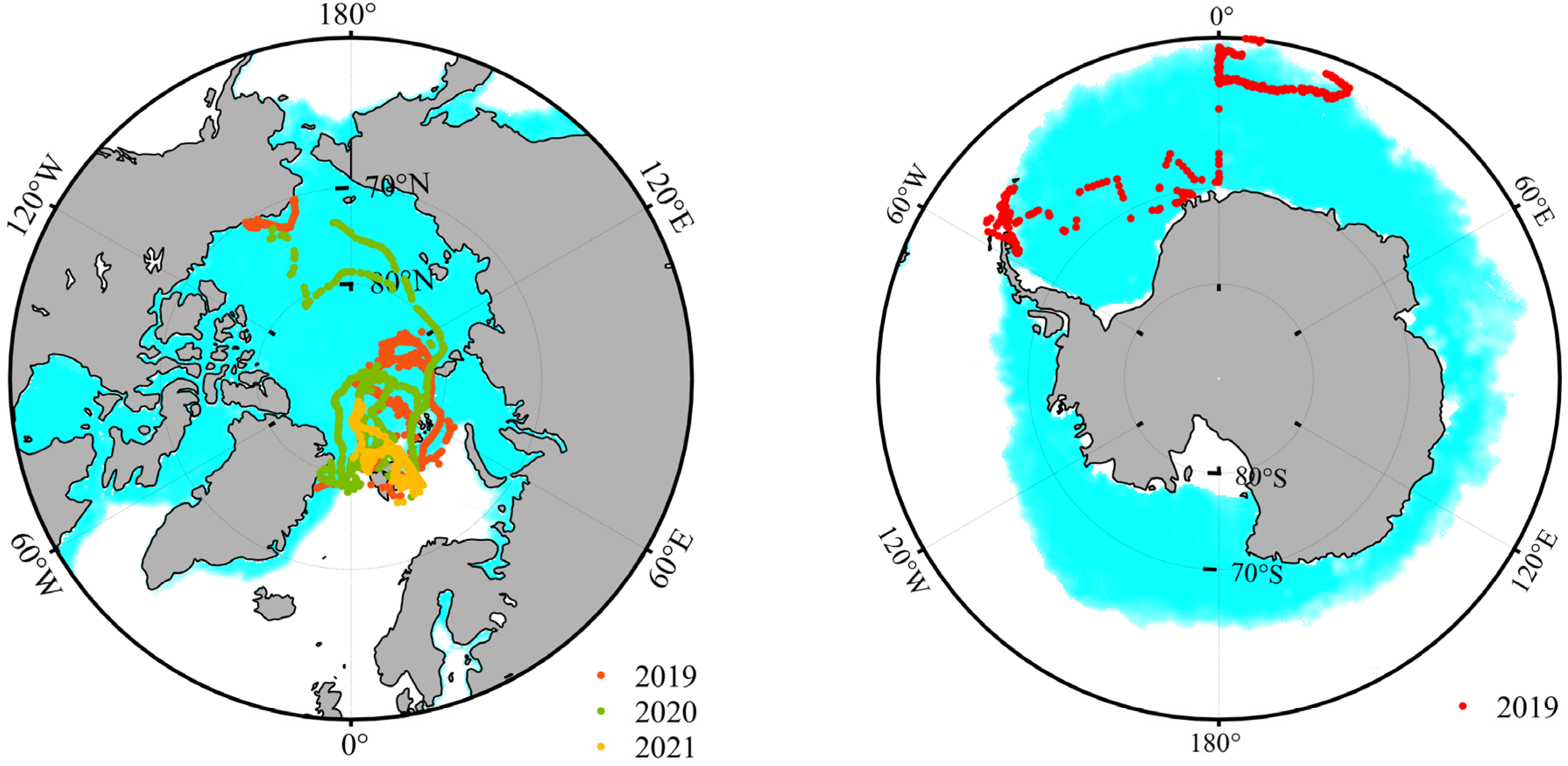
2.3. Ship-Based Sea Ice Cover Observations
3. Methods
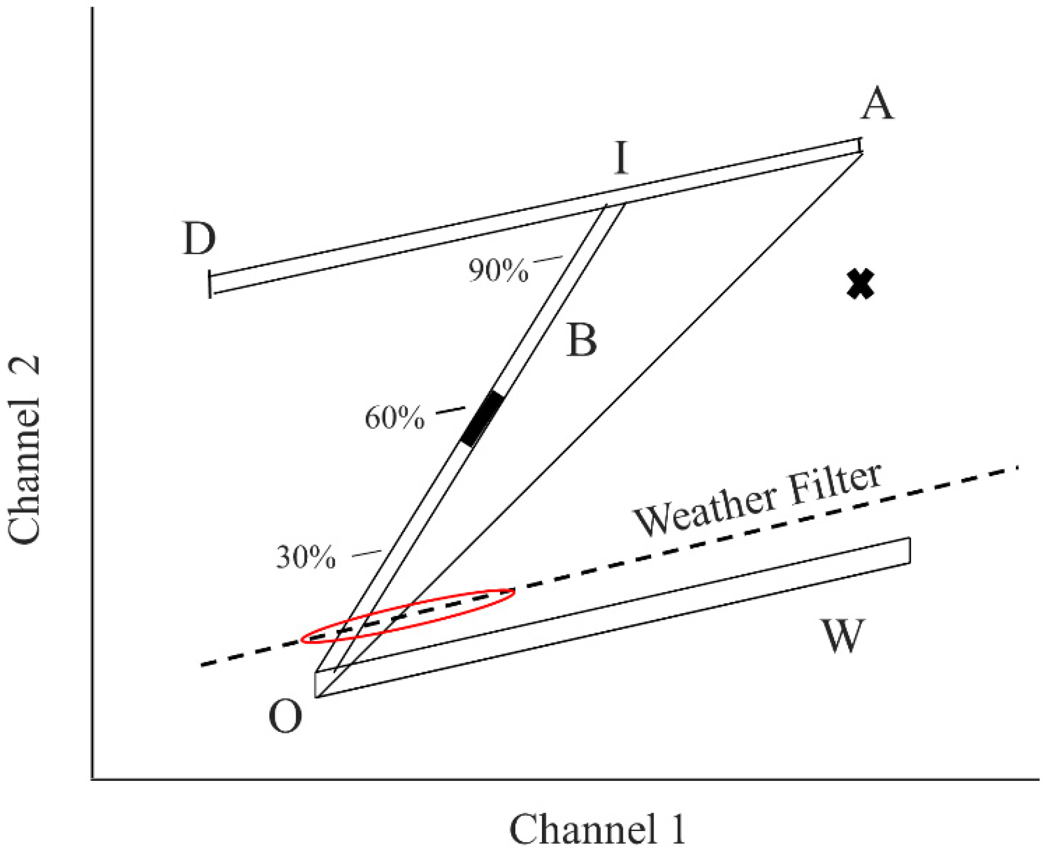
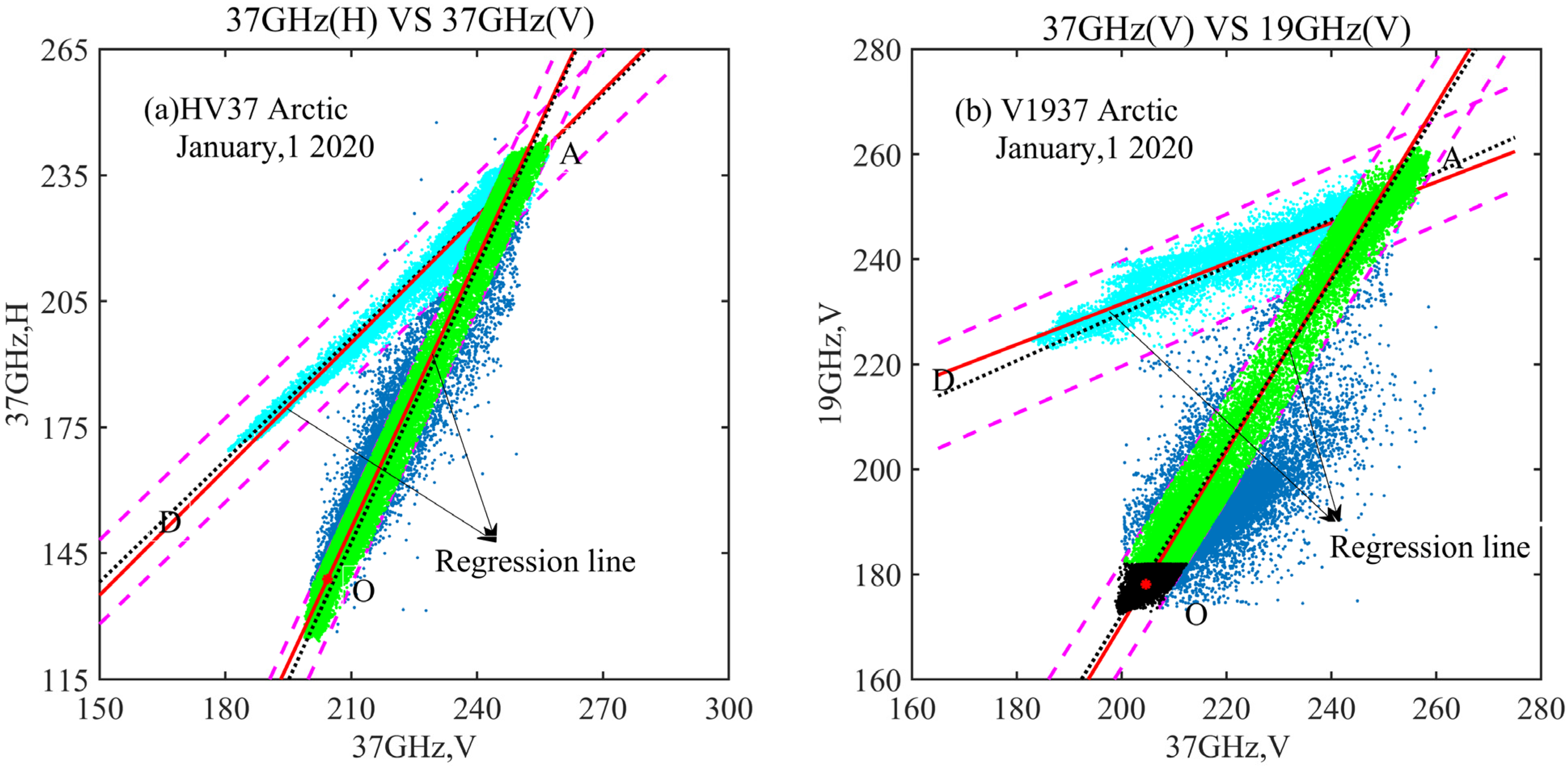
3.1. Basic BT Algorithm Technique
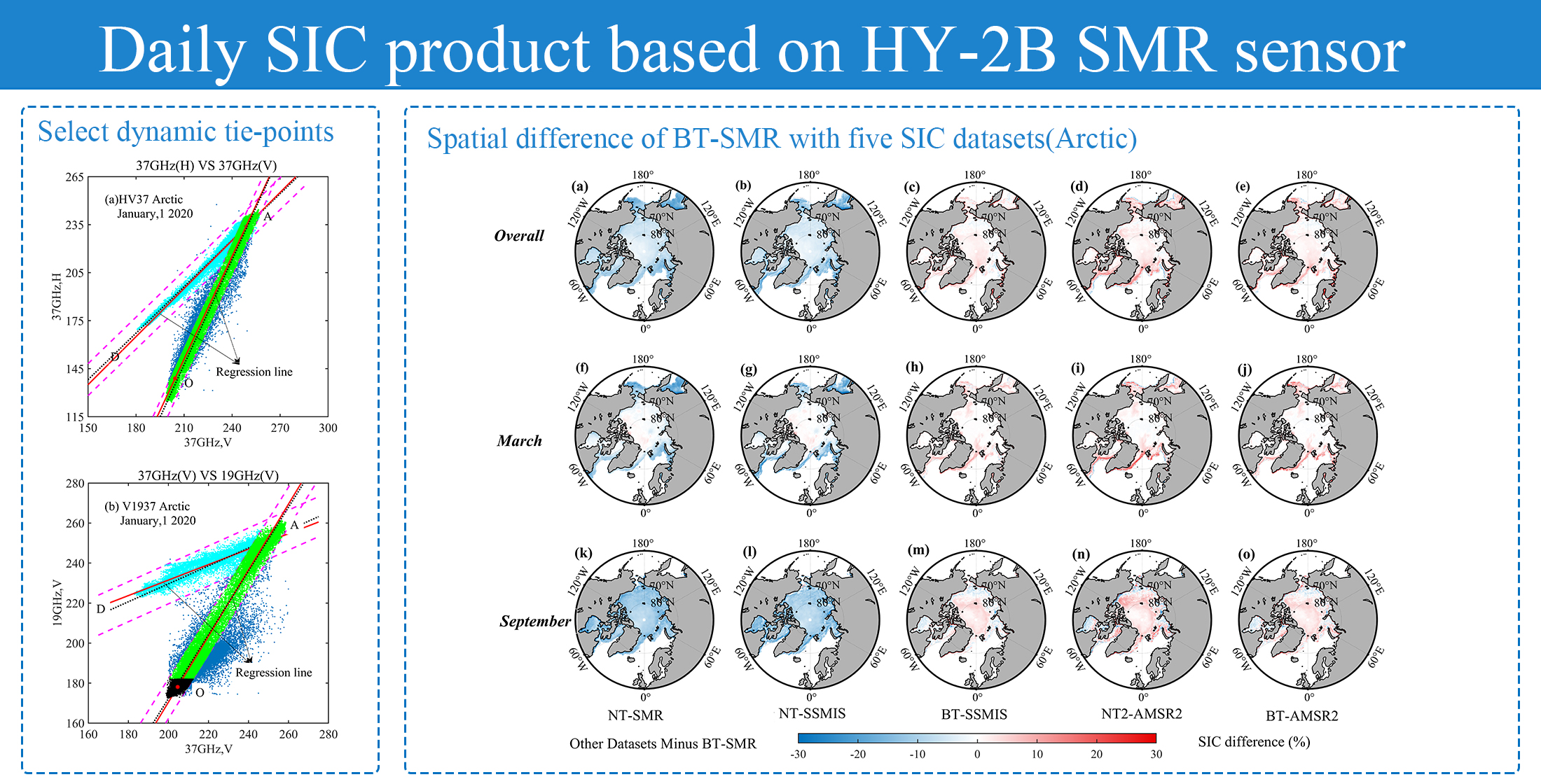
3.2. Choice of Tie-Points
3.3. Weather Filters
- (1)
- The SIC is set to 0% if (Arctic) or (Antarctic), which mainly removes the effects of liquid water and ice crystals in the clouds.
- (2)
- The SIC is set to 0% if (Arctic) or () (Antarctic), which mainly removes the effect of water vapor over open water.
3.4. Land Spillover Correction
4. Results
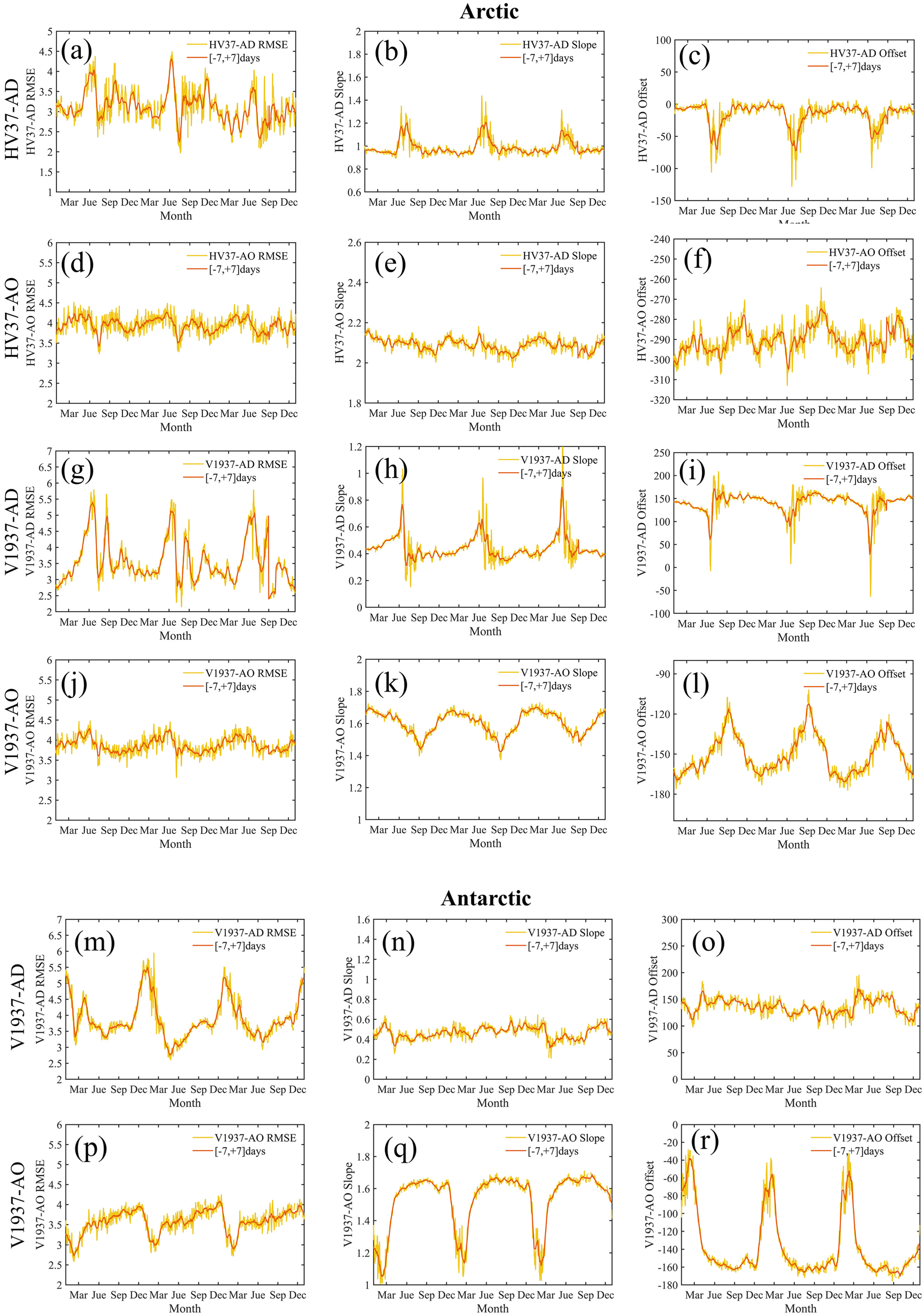
4.1. BT Algorithm Tie-Points Time Series Analysis
4.2. Comparisons of the BT-SMR SIC Products
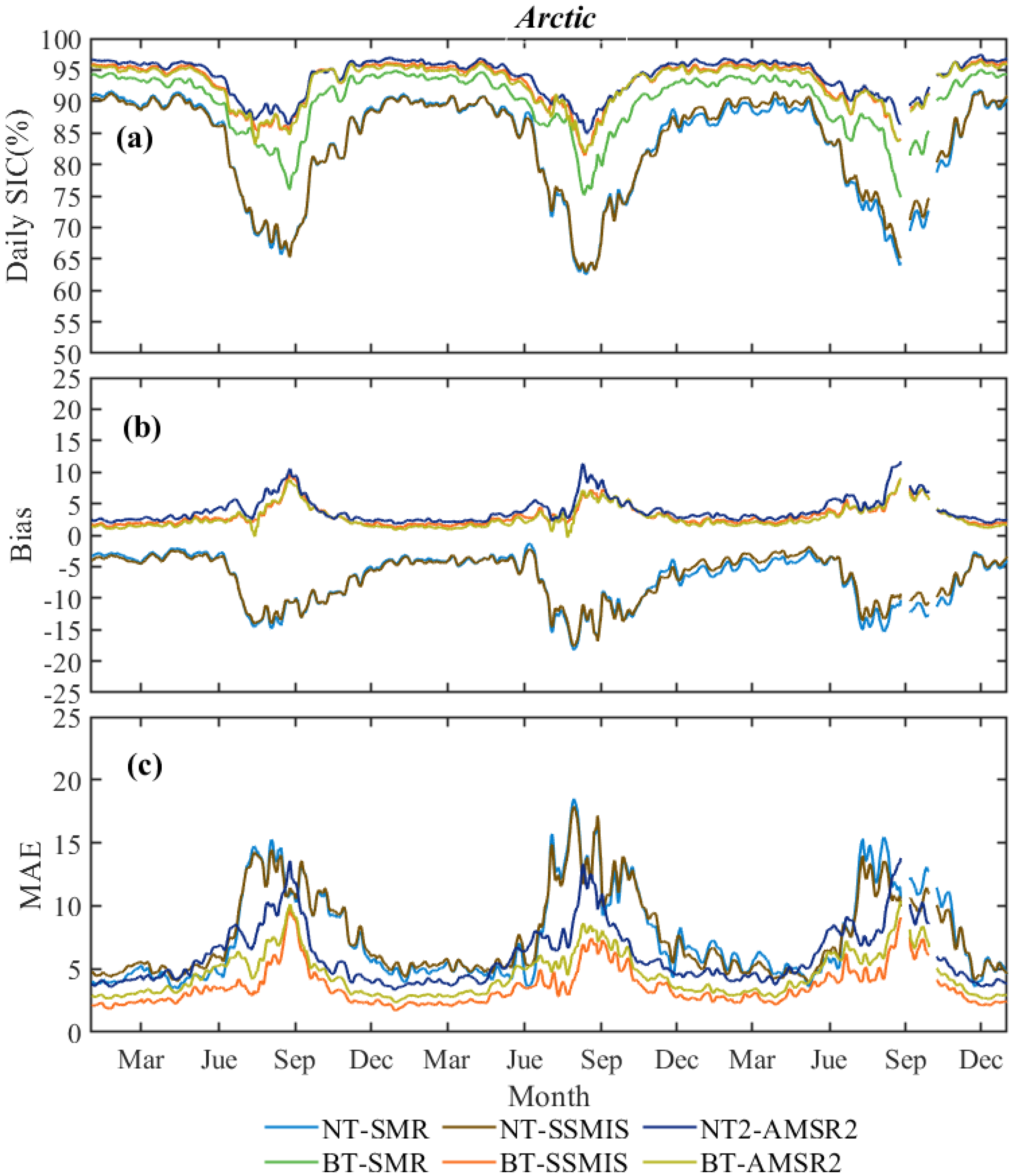
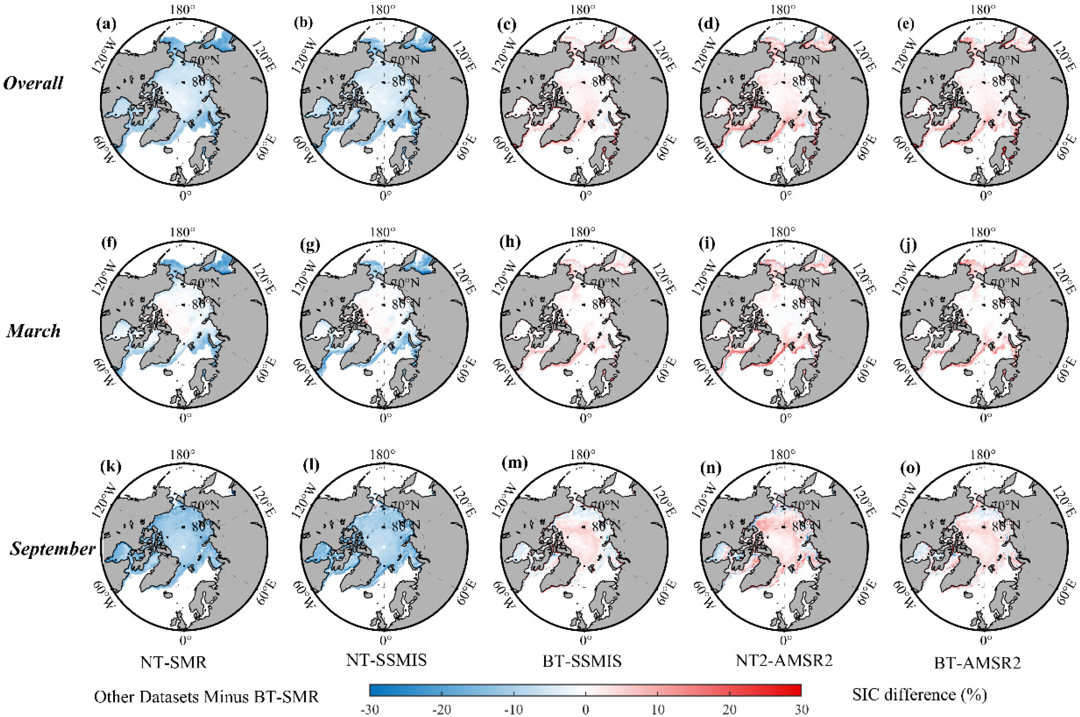
4.2.1. Arctic SIC and Spatial Distribution Differences
4.2.2. Antarctic SIC and Spatial Distribution Differences
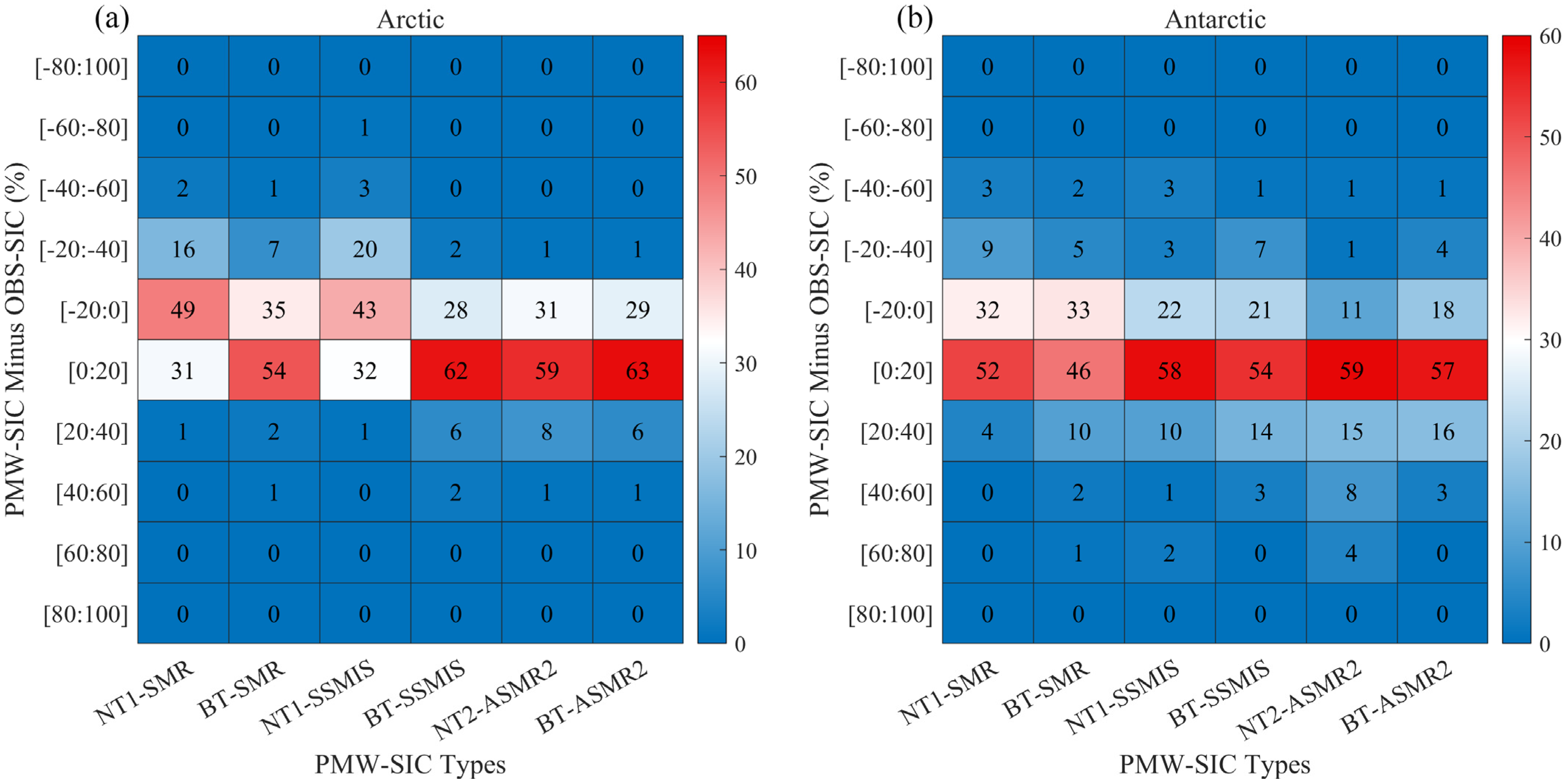
4.2.3. Assessing SIC Differences by Intervals
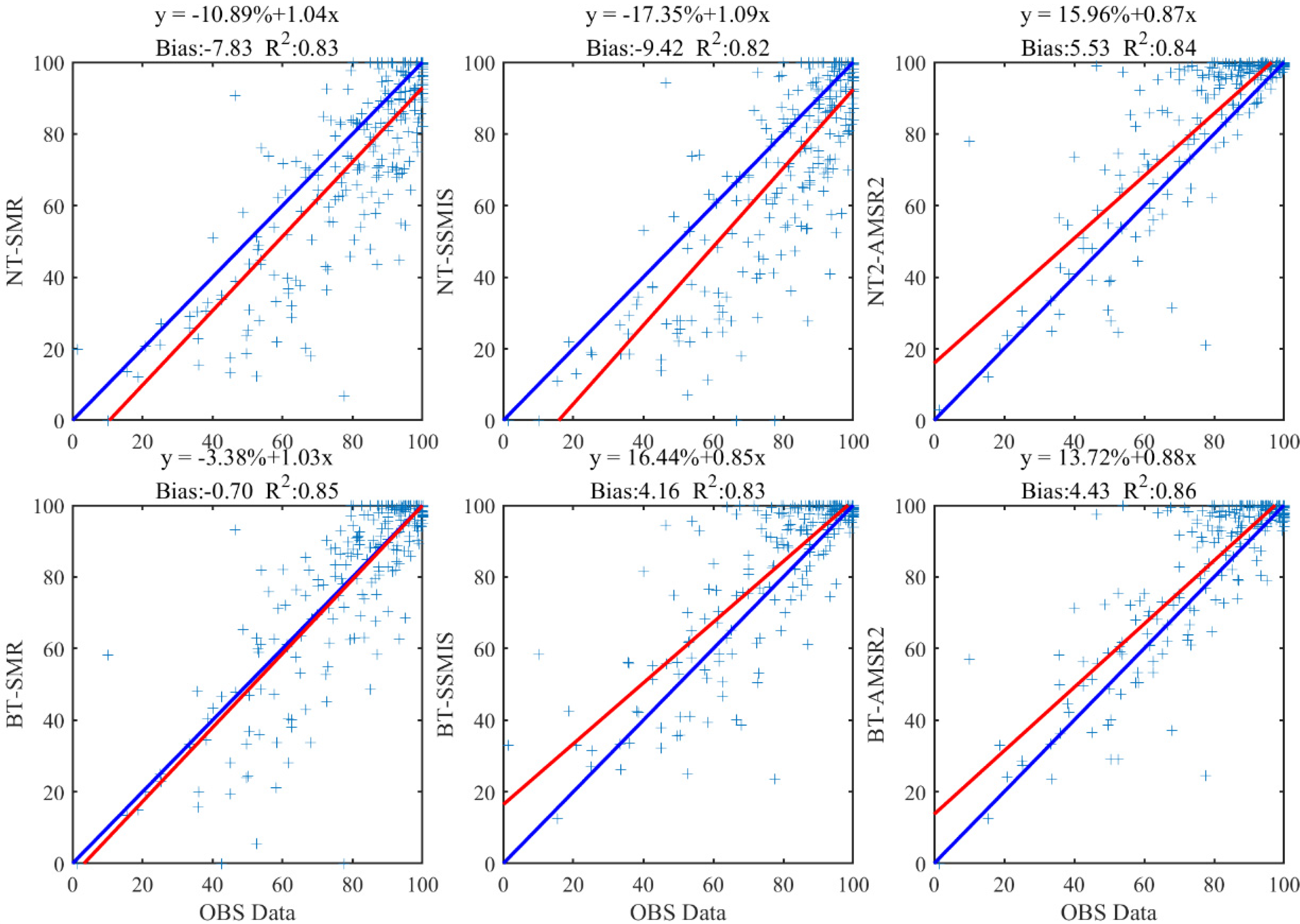
4.3. Inter-Comparison of the Ship-Based SIC
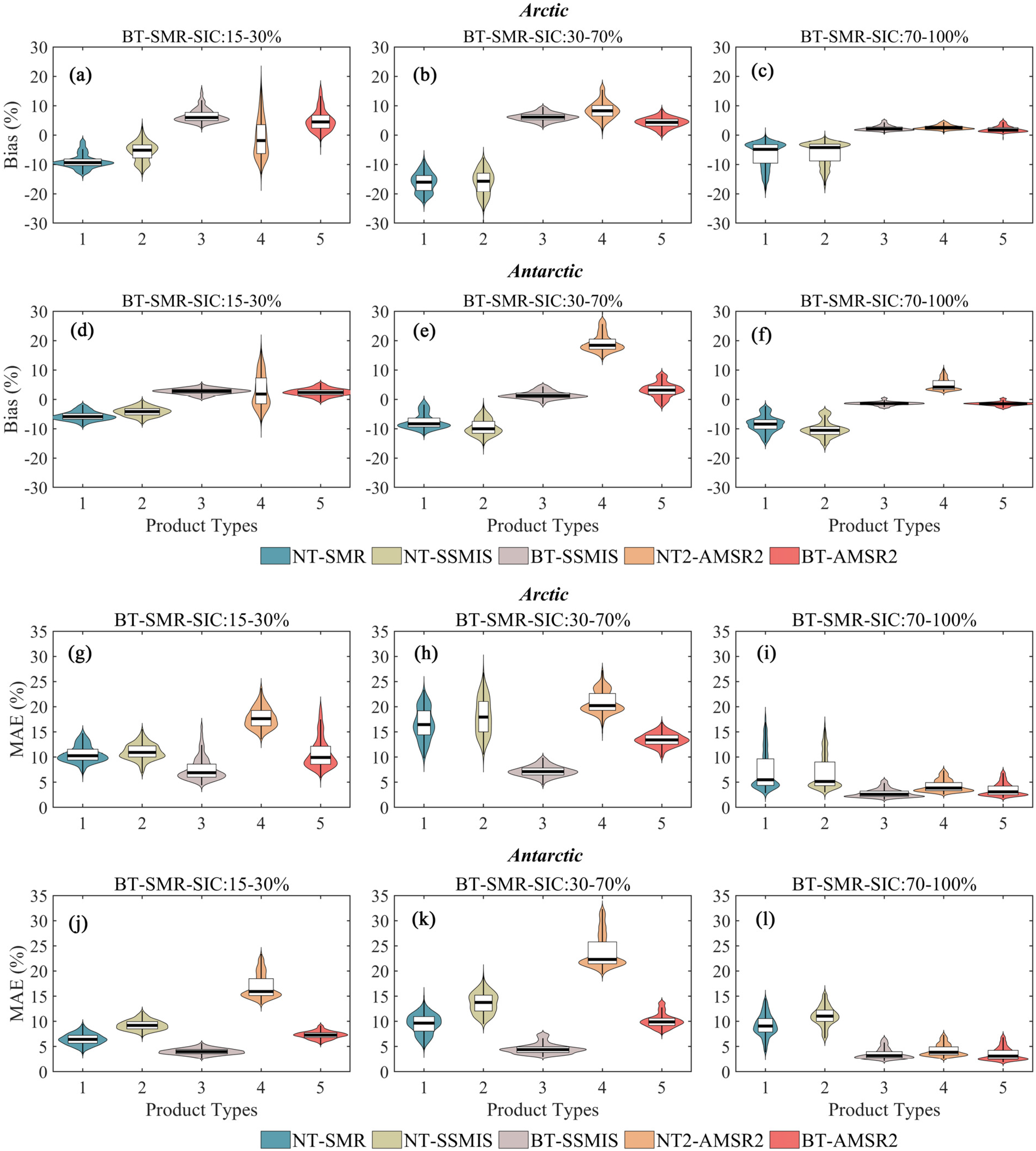
4.3.1. Arctic
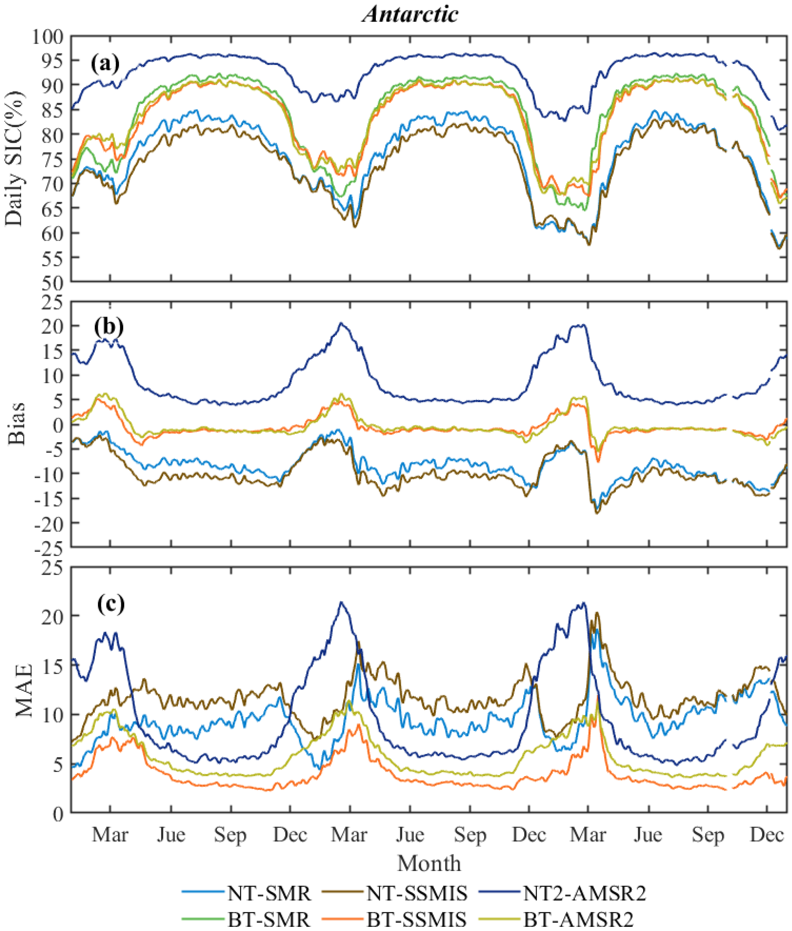
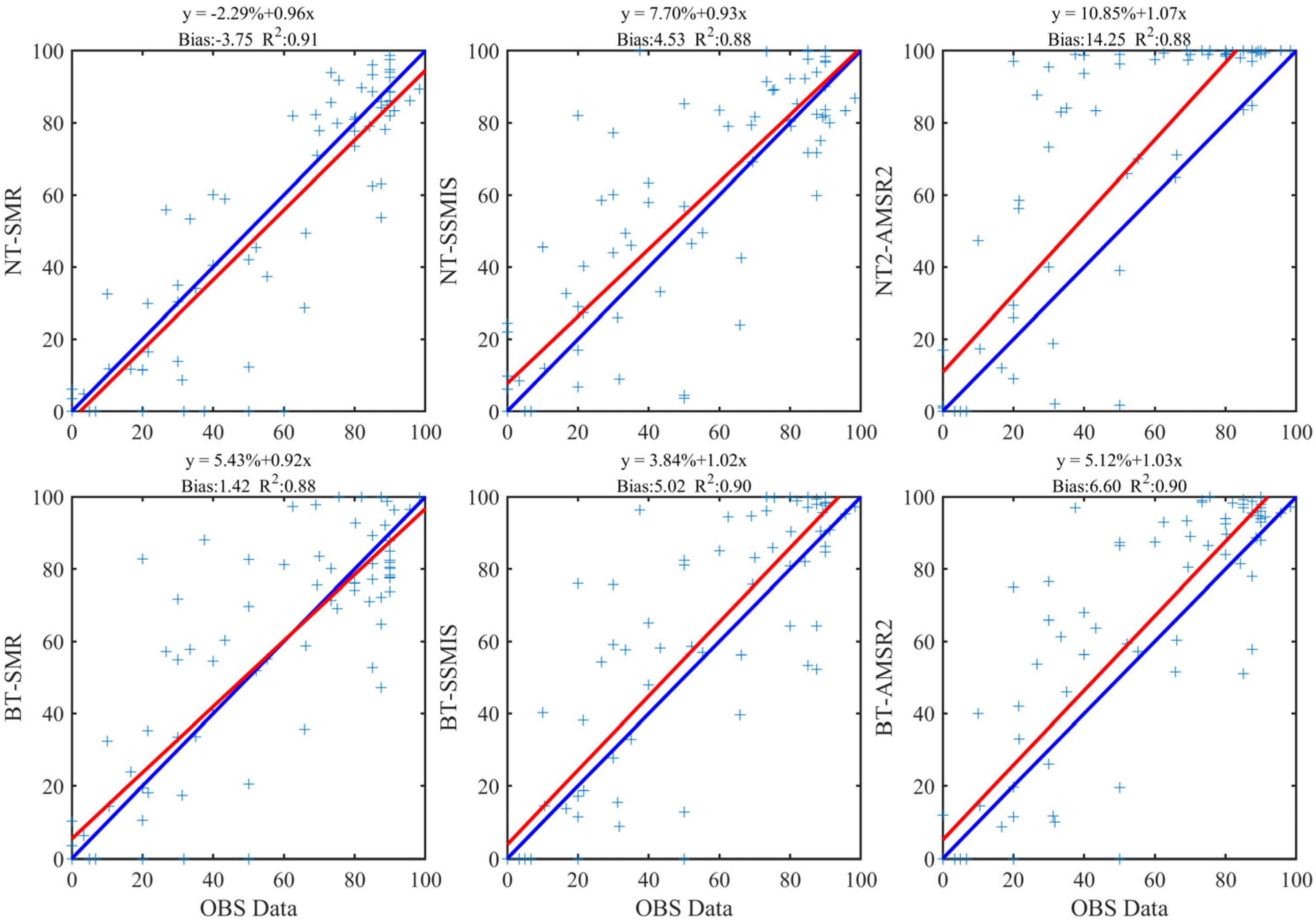
4.3.2. Antarctic
5. Discussion
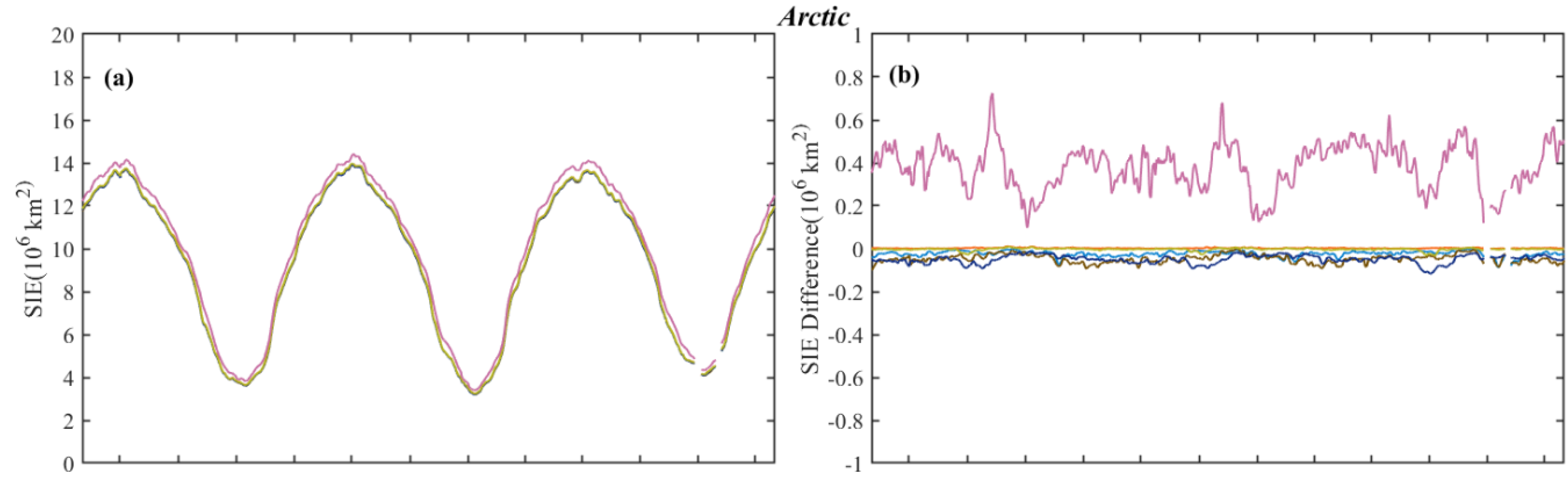
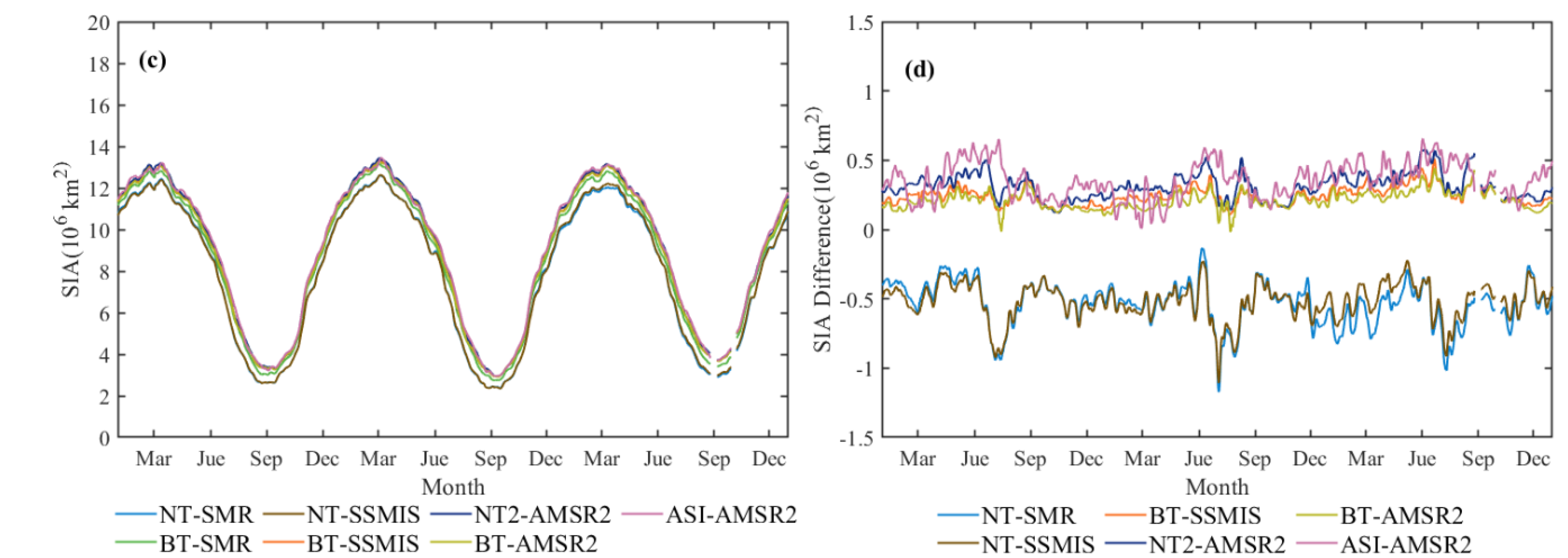
5.1. Arctic SIE and SIA Time Series Analysis
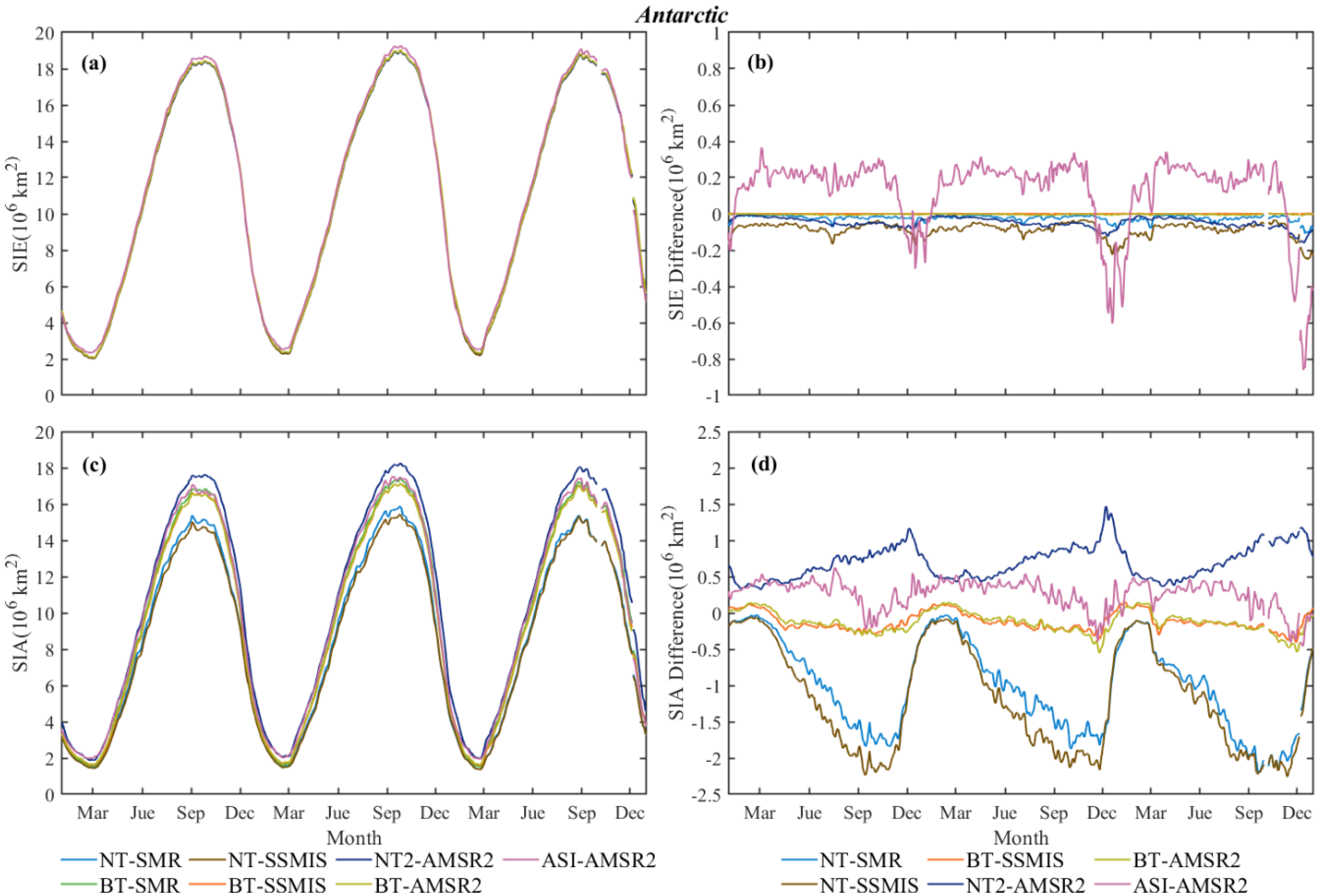
5.2. Antarctic SIE and SIA Time Series Analysis
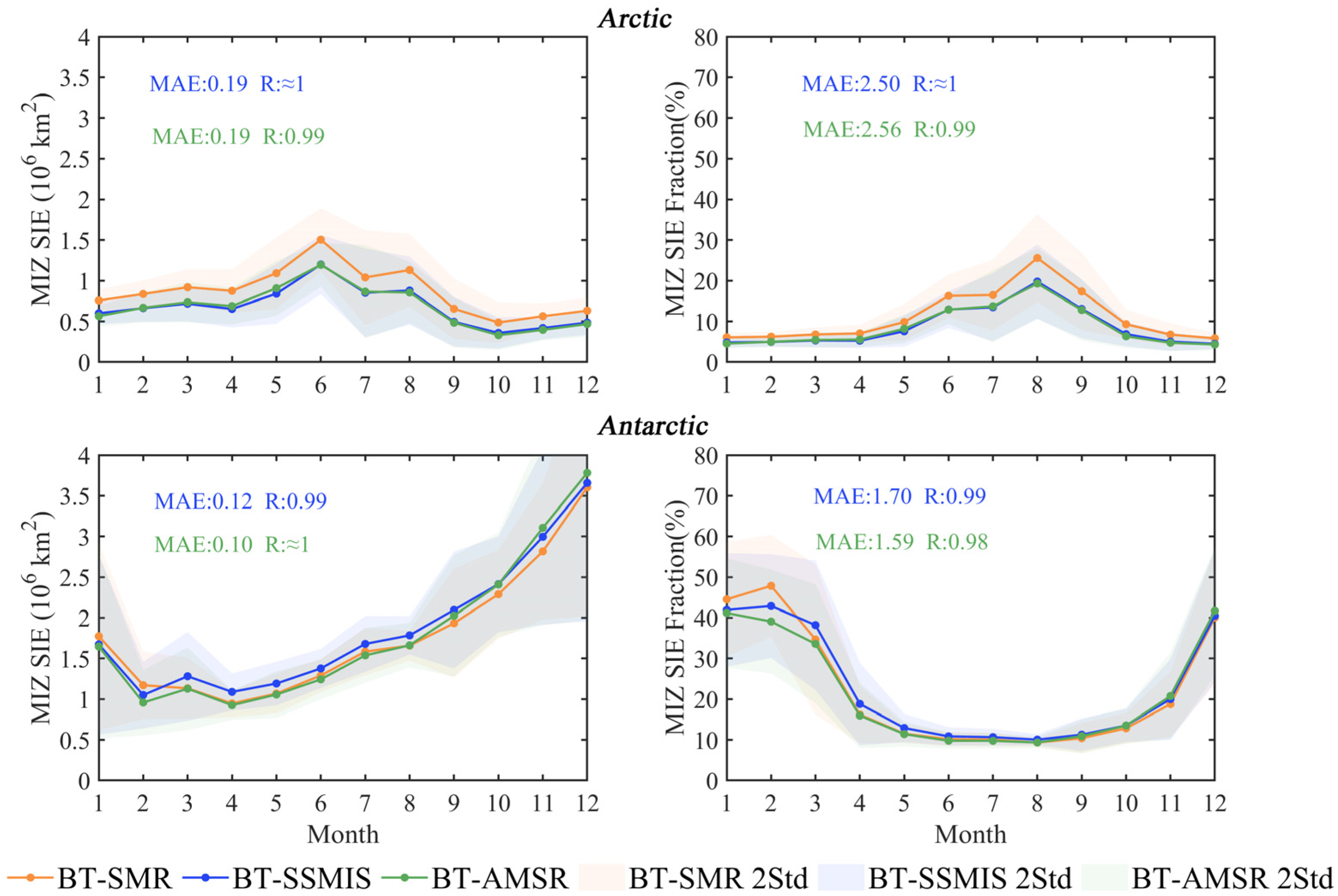
5.3. Assessing MIZ SIE with Different BT SIC Products
6. Conclusions
Author Contributions
Funding
Data Availability Statement
Conflicts of Interest
References
- Serreze, M.C.; Barrett, A.P.; Stroeve, J.C.; Kindig, D.N.; Holland, M.M. The emergence of surface-based Arctic amplification. Cryosphere 2009, 3, 11–19. [Google Scholar] [CrossRef]
- Manabe, S.; Wetherald, R.T. The effects of doubling the CO2 concentration on the climate of a general circulation model. J. Atmos. Sci. 1975, 32, 3–15. [Google Scholar] [CrossRef]
- Ingels, J.; Aronson, R.B.; Smith, C.R.; Baco, A.; Bik, H.M.; Blake, J.A.; Brandt, A.; Cape, M.; Demaster, D.; Dolan, E. Antarctic ecosystem responses following ice-shelf collapse and iceberg calving: Science review and future research. Wiley Interdiscip. Rev. Clim. Chang. 2021, 12, e682. [Google Scholar] [CrossRef]
- Cheung, H.H.; Keenlyside, N.; Omrani, N.-E.; Zhou, W. Remarkable link between projected uncertainties of Arctic sea-ice decline and winter Eurasian climate. Adv. Atmos. Sci. 2018, 35, 38–51. [Google Scholar] [CrossRef]
- Xu, S.; Zhou, L.; Liu, J.; Lu, H.; Wang, B. Data Synergy between Altimetry and L-Band Passive Microwave Remote Sensing for the Retrieval of Sea Ice Parameters—A Theoretical Study of Methodology. Remote Sens. 2017, 9, 1079. [Google Scholar] [CrossRef]
- Kwok, R. Arctic sea ice thickness, volume, and multiyear ice coverage: Losses and coupled variability (1958–2018). Environ. Res. Lett. 2018, 13, 105005. [Google Scholar] [CrossRef]
- Kinnard, C.; Zdanowicz, C.M.; Fisher, D.A.; Isaksson, E.; de Vernal, A.; Thompson, L.G. Reconstructed changes in Arctic sea ice over the past 1450 years. Nature 2011, 479, 509–512. [Google Scholar] [CrossRef] [PubMed]
- Yu, L.; Zhong, S.; Winkler, J.A.; Zhou, M.; Lenschow, D.H.; Li, B.; Wang, X.; Yang, Q. Possible connections of the opposite trends in Arctic and Antarctic sea-ice cover. Sci. Rep. 2017, 7, 45804. [Google Scholar] [CrossRef]
- Stroeve, J.C.; Markus, T.; Boisvert, L.; Miller, J.; Barrett, A. Changes in Arctic melt season and implications for sea ice loss. Geophys. Res. Lett. 2014, 41, 1216–1225. [Google Scholar] [CrossRef]
- Tikhonov, V.; Raev, M.; Sharkov, E.; Boyarskii, D.; Repina, I.; Komarova, N.Y. Satellite microwave radiometry of sea ice of polar regions: A review. Izv. Atmos. Ocean. Phys. 2016, 52, 1012–1030. [Google Scholar] [CrossRef]
- Alekseeva, T.; Tikhonov, V.; Frolov, S.; Repina, I.; Raev, M.; Sokolova, J.; Sharkov, E.; Afanasieva, E.; Serovetnikov, S. Comparison of Arctic Sea Ice concentrations from the NASA team, ASI, and VASIA2 algorithms with summer and winter ship data. Remote Sens. 2019, 11, 2481. [Google Scholar] [CrossRef]
- Parkinson, C.L.; Comiso, J.C.; Zwally, H.J.; Cavalieri, D.J.; Gloersen, P.; Campbell, W.J. Arctic Sea Ice, 1973–1976: Satellite Passive-Microwave Observations; Scientific and Technical Information Branch, National Aeronautics and Space Administration, 1987. Available online: https://ntrs.nasa.gov/citations/19870015437 (accessed on 6 December 2022).
- Zwally, H.J. Antarctic Sea Ice, 1973–1976: Satellite Passive-Microwave Observations; Scientific and Technical Information Branch, National Aeronautics and Space, 1983; Volume 459. Available online: https://ntrs.nasa.gov/citations/19840002650 (accessed on 6 December 2022).
- Chen, Y.; Zhao, X.; Pang, X.; Ji, Q. Daily sea ice concentration product based on brightness temperature data of FY-3D MWRI in the Arctic. Big Earth Data 2022, 6, 164–178. [Google Scholar] [CrossRef]
- Chen, Y.; Zhao, X.; Lei, R.; Wu, S.; Liu, Y.; Fan, P.; Ji, Q.; Zhang, P.; Pang, X. A new Sea Ice Concentration Product in the Polar regions Derived from the FengYun-3 MWRI Sensors. Earth Syst. Sci. Data Discuss 2022, 1–25. [Google Scholar] [CrossRef]
- Zhao, X.; Chen, Y.; Kern, S.; Qu, M.; Ji, Q.; Fan, P.; Liu, Y. Sea Ice Concentration Derived From FY-3D MWRI and Its Accuracy Assessment. IEEE Trans. Geosci. Remote Sens. 2021, 60, 1–18. [Google Scholar] [CrossRef]
- Shi, L.; Liu, S.; Shi, Y.; Ao, X.; Wang, Q. Sea Ice Concentration Products over Polar Regions with Chinese FY3C/MWRI Data. Remote Sens. 2021, 13, 2174. [Google Scholar] [CrossRef]
- Witze, A. Ageing satellites put crucial sea-ice climate record at risk. Nature 2017, 551, 13–14. [Google Scholar] [CrossRef]
- Cavalieri, D.J.; Gloersen, P.; Campbell, W.J. Determination of sea ice parameters with the NIMBUS 7 SMMR. J. Geophys. Res. Atmos. 1984, 89, 5355–5369. [Google Scholar] [CrossRef]
- Comiso, J.C. Enhanced Sea Ice Concentrations from Passive Microwave Data; NASA Goddard Space Flight Center: Greenbelt, MD, USA, 2007.
- Comiso, J. SSM/I Sea Ice Concentrations Using the Bootstrap Algorithm; National Aeronautics and Space Administration, Goddard Space Flight Center: Greenbelt, MD, USA, 1995; p. 1380. [CrossRef]
- Comiso, J.C.; Sullivan, C.W. Satellite microwave and in situ observations of the Weddell Sea ice cover and its marginal ice zone. J. Geophys. Res. Ocean. 1986, 91, 9663–9681. [Google Scholar] [CrossRef]
- Comiso, J.C. Characteristics of Arctic winter sea ice from satellite multispectral microwave observations. J. Geophys. Res. Ocean. 1986, 91, 975–994. [Google Scholar] [CrossRef]
- Smith, D.M. Extraction of winter total sea-ice concentration in the Greenland and Barents Seas from SSM/I data. Int. J. Remote Sens. 1996, 17, 2625–2646. [Google Scholar] [CrossRef]
- Lavergne, T.; Sørensen, A.; Kern, S.; Tonboe, R.; Notz, D.; Aaboe, S.; Bell, L.; Dybkjaer, G.; Eastwood, S.; Gabarro, C.; et al. Version 2 of the EUMETSAT OSI SAF and ESA CCI sea-ice concentration climate data records. Cryosphere 2019, 13, 49–78. [Google Scholar] [CrossRef]
- Tonboe, R.; Eastwood, S.; Lavergne, T.; Sørensen, A.; Rathmann, N.; Dybkjaer, G.; Pedersen, L.; Høyer, J.; Kern, S. The EUMETSAT sea ice concentration climate data record. Cryosphere 2016, 10, 2275–2290. [Google Scholar] [CrossRef]
- Brucker, L.; Cavalieri, D.J.; Markus, T.; Ivanoff, A. NASA Team 2 Sea Ice Concentration Algorithm Retrieval Uncertainty. Geosci. Remote Sens. 2014, 52, 7336–7352. [Google Scholar] [CrossRef]
- Markus, T.; Cavalieri, D. An enhancement of the NASA Team sea ice algorithm. Geosci. Remote Sens. IEEE Trans. 2000, 38, 1387–1398. [Google Scholar] [CrossRef]
- Spreen, G.; Kaleschke, L.; Heygster, G. Sea ice remote sensing using AMSR-E 89-GHz channels. J. Geophys. Res. Ocean. 2008, 113. [Google Scholar] [CrossRef]
- Svendsen, E.; Matzler, C.; Grenfell, T.C. A model for retrieving total sea ice concentration from a spaceborne dual-polarized passive microwave instrument operating near 90 GHz. Int. J. Remote Sens. 1987, 8, 1479–1487. [Google Scholar] [CrossRef]
- Kern, S.; Lavergne, T.; Notz, D.; Pedersen, L.T.; Tonboe, R.T.; Saldo, R.; Sørensen, A.M. Satellite passive microwave sea-ice concentration data set intercomparison: Closed ice and ship-based observations. Cryosphere 2019, 13, 3261–3307. [Google Scholar] [CrossRef]
- Comiso, J.C.; Meier, W.N.; Gersten, R. Variability and trends in the Arctic Sea ice cover: Results from different techniques. J. Geophys. Res. Ocean. 2017, 122, 6883–6900. [Google Scholar] [CrossRef]
- Ivanova, N.; Johannessen, O.M.; Pedersen, L.T.; Tonboe, R.T. Retrieval of Arctic Sea Ice Parameters by Satellite Passive Microwave Sensors: A Comparison of Eleven Sea Ice Concentration Algorithms. IEEE Trans. Geosci. Remote Sens. 2014, 52, 7233–7246. [Google Scholar] [CrossRef]
- Pang, X.; Pu, J.; Zhao, X.; Ji, Q.; Qu, M.; Cheng, Z. Comparison between AMSR2 Sea Ice Concentration Products and Pseudo-Ship Observations of the Arctic and Antarctic Sea Ice Edge on Cloud-Free Days. Remote Sens. 2018, 10, 317. [Google Scholar]
- Wiebe, H.; Heygster, G.; Markus, T. Comparison of the ASI Ice Concentration Algorithm With Landsat-7 ETM+ and SAR Imagery. IEEE Trans. Geosci. Remote Sens. 2009, 47, 3008–3015. [Google Scholar] [CrossRef]
- Meier, W.N. Comparison of passive microwave ice concentration algorithm retrievals with AVHRR imagery in arctic peripheral seas. IEEE Trans. Geosci. Remote Sens. 2005, 43, 1324–1337. [Google Scholar] [CrossRef]
- Agnew, T.; Howell, S. The use of operational ice charts for evaluating passive microwave ice concentration data. Atmos. Ocean. 2003, 41, 317–331. [Google Scholar] [CrossRef]
- Agnew, T.A.; Howell, S. Comparison of digitized Canadian ice charts and passive microwave sea-ice concentrations. In Proceedings of the IEEE International Geoscience and Remote Sensing Symposium, Kuala Lumpur, Malaysia, 17–22 July 2002; pp. 231–233. [Google Scholar]
- Zong, F.; Zhang, S.; Chen, P.; Yang, L.; Shao, Q.; Zhao, J.; Wei, L. Evaluation of Sea Ice Concentration Data Using Dual-Polarized Ratio Algorithm in Comparison With Other Satellite Passive Microwave Sea Ice Concentration Data Sets and Ship-Based Visual Observations. Front. Environ. Sci. 2022, 10, 278. [Google Scholar] [CrossRef]
- Beitsch, A.; Kern, S.; Kaleschke, L. Comparison of SSM/I and AMSR-E Sea Ice Concentrations With ASPeCt Ship Observations Around Antarctica. IEEE Trans. Geosci. Remote Sens. 2015, 53, 1985–1996. [Google Scholar] [CrossRef]
- Ozsoy-Cicek, B.; Xie, H.; Ackley, S.; Ye, K. Antarctic summer sea ice concentration and extent: Comparison of ODEN 2006 ship observations, satellite passive microwave and NIC sea ice charts. Cryosphere 2009, 3, 1–9. [Google Scholar] [CrossRef]
- Knuth, M.A.; Ackley, S.F. Summer and early-fall sea-ice concentration in the Ross Sea: Comparison of in situ ASPeCt observations and satellite passive microwave estimates. Ann. Glaciol. 2006, 44, 303–309. [Google Scholar] [CrossRef]
- Ivanova, N.; Pedersen, L.T.; Tonboe, R.T.; Kern, S.; Heygster, G.; Lavergne, T.; Sørensen, A.; Saldo, R.; Dybkjær, G.; Brucker, L.J.T.C. Inter-comparison and evaluation of sea ice algorithms: Towards further identification of challenges and optimal approach using passive microwave observations. Cryosphere 2015, 9, 1797–1817. [Google Scholar] [CrossRef]
- Kern, S.; Lavergne, T.; Pedersen, L.; Tonboe, R.; Bell, L.; Meyer, M.; Zeigermann, L. Satellite passive microwave sea-ice concentration data set intercomparison using Landsat data. Cryosphere 2022, 16, 349–378. [Google Scholar] [CrossRef]
- Cavalieri, D.; Parkinson, C.; Gloersen, P.; Zwally, H. Sea Ice Concentrations from Nimbus-7 SMMR and DMSP SSM/ISSMI Passive Microwave Data, Version 1 [Data Set]; NASA National Snow and Ice Data Center Distributed Active Archive Center: Boulder, CO, USA, 1996. [CrossRef]
- Comiso, J. Bootstrap Sea Ice Concentrations from Nimbus-7 SMMR and DMSP SSM/I-SSMIS, Version 3 [Data Set]; NASA National Snow and Ice Data Center Distributed Active Archive Center: Boulder, CO, USA, 2017. [CrossRef]
- Worby, A.; Comiso, J.C. Studies of the Antarctic sea ice edge and ice extent from satellite and ship observations. Remote Sens. Environ. 2004, 92, 98–111. [Google Scholar] [CrossRef]
- Comiso, J.C.; Cavalieri, D.J.; Parkinson, C.L.; Gloersen, P. Passive microwave algorithms for sea ice concentration: A comparison of two techniques. Remote Sens. Environ. 1997, 60, 357–384. [Google Scholar] [CrossRef]
- Matzler, C.; Ramseier, R.; Svendsen, E. Polarization effects in seaice signatures. IEEE J. Ocean. Eng. 1984, 9, 333–338. [Google Scholar] [CrossRef]
- Cavalieri, D.J.; Parkinson, C.L.; Gloersen, P.; Zwally, H.J. Arctic and Antarctic Sea Ice Concentrations from Multichannel Passive-Microwave Satellite Data Sets: October 1978–September 1995 User’s Guide. 1997. Available online: https://ntrs.nasa.gov/citations/19980076134 (accessed on 6 December 2022).
- Andersen, S.; Tonboe, R.; Kaleschke, L.; Heygster, G.; Pedersen, L. Intercomparison of passive microwave sea ice concentration retrievals over the high-concentration Arctic sea ice. J. Geophys. Res. 2007, 112. [Google Scholar] [CrossRef]


| Sensor | Platform | Frequencies in GHz | View Angle | Operation Date |
|---|---|---|---|---|
| ESMR | Nimbus-5 | 19.4 | 0–50° | 1972–1976 |
| SMMR | Nimbus-7 | 6.6, 10.7, 18.0, 21.0, 37.0 | 50.2° | 1978–1987 |
| SSM/I | DMSPF8-F11 13–F15 | 19.4, 22.2, 37.0, 85.5 | 53.1° | 1987–2009 |
| SSMIS | DMSP F16–F19 | 19.4, 22.2, 37.0, 91.7 | 53.1° | 2003–today |
| AMSR-E | Aqua | 6.9, 10.7, 18.7, 23.8, 36.5, 89.0 | 55° | 2002–2011 |
| AMSR2 | GCOW-W1 | 6.9, 7.3, 10.7, 18.7, 23.8, 36.5, 89.0 | 55° | 2012–today |
| SMR | HY-2B | 6.4, 10.7, 18.7, 23.8, 37.0 | 53° | 2018–today |
| MWRI | FY-3B/C/D | 10.7, 18.7, 23.8, 36.5, 89.0 | 52° | 2010–today |
| Configuration Parameter | Values | ||||
|---|---|---|---|---|---|
| Frequency (GHz) | 6.925 | 10.7 | 18.7 | 23.8 | 37.0 |
| Polarization | V H | VH | VH | V | VH |
| Bandwidth (MHz) | 350 | 100 | 200 | 400 | 1000 |
| Sensitivity (K) | 0.5 | 0.6 | 0.5 | 0.5 | 0.8 |
| Calibration Error (K) | 1 | ||||
| Ground Resolution (km) | 90 × 150 | 70 × 110 | 36 × 60 | 30 × 52 | 20 × 35 |
| Dynamic Range (K) | 3–350 | ||||
| Scan Mode | Conical scanning | ||||
| Orbit Width (km) | 1600 | ||||
| View angle (°) | 53 | ||||
| Datasets | Source | Period | Sensor | Algorithm | Resolution (km) |
|---|---|---|---|---|---|
| BT-SMR | This study | 2019–2021 | SMR | BT | 25 |
| NT-SMR | NSOAS | 2019–2021 | SMR | NT | 25 |
| NT-SSMIS | NSIDC | 2019–2021 | SSMIS | NT | 25 |
| BT-SSMIS | NSIDC | 2019–2021 | SSMIS | BT | 25 |
| NT2-AMSR2 | NSIDC | 2019–2021 | AMSR2 | NT2 | 25 |
| BT-AMSR2 | NSIDC | 2019–2021 | AMSR2 | BT | 25 |
| ASI-AMSR2 | Bremen | 2019–2021 | ASMR2 | ASI | 6.25 |
| ID | NT-SMR | NT-SSMIS | BT-SSMIS | NT2-AMSR | BT-AMSR | |
|---|---|---|---|---|---|---|
| Overall | Bias | −8.87 | −7.96 | 2.89 | 3.26 | 3.25 |
| MAE | 9.00 | 8.20 | 3.64 | 4.71 | 4.16 | |
| RMSE | 10.59 | 10.35 | 6.74 | 7.55 | 7.48 | |
| R2 | 0.97 | 0.96 | 0.96 | 0.95 | 0.95 | |
| March | Bias | −5.38 | −4.68 | 2.01 | 2.06 | 2.11 |
| MAE | 5.87 | 5.36 | 2.33 | 3.44 | 2.77 | |
| RMSE | 8.71 | 8.50 | 4.09 | 5.92 | 5.13 | |
| R2 | 0.97 | 0.97 | 0.98 | 0.96 | 0.97 | |
| September | Bias | −11.91 | −11.34 | 1.98 | 2.14 | 2.18 |
| MAE | 12.12 | 11.57 | 4.43 | 6.06 | 4.86 | |
| RMSE | 13.21 | 12.96 | 8.21 | 9.08 | 8.37 | |
| R2 | 0.96 | 0.95 | 0.91 | 0.90 | 0.91 |
| ID | NT-SMR | NT-SSMIS | BT-SSMIS | NT2-AMSR | BT-AMSR | |
|---|---|---|---|---|---|---|
| Overall | Bias | −8.11 | −10.89 | −0.75 | 5.17 | −0.12 |
| MAE | 8.25 | 11.03 | 1.93 | 5.81 | 2.50 | |
| RMSE | 8.79 | 11.61 | 2.64 | 7.22 | 3.62 | |
| R2 | 0.99 | 0.98 | 0.99 | 0.97 | 0.99 | |
| March | Bias | −7.86 | −12.43 | −1.88 | 9.23 | 0.68 |
| MAE | 9.97 | 13.84 | 5.83 | 10.72 | 6.66 | |
| RMSE | 11.65 | 15.53 | 7.61 | 13.66 | 8.92 | |
| R2 | 0.91 | 0.90 | 0.93 | 0.89 | 0.90 | |
| September | Bias | −7.74 | −10.51 | 0.96 | 4.22 | −0.24 |
| MAE | 7.95 | 10.72 | 2.23 | 4.95 | 2.67 | |
| RMSE | 8.94 | 11.72 | 2.95 | 7.04 | 3.65 | |
| R2 | 0.98 | 0.97 | 0.99 | 0.97 | 0.99 |
| ID | NT-SMR | BT-SMR | NT-SSMIS | BT-SSMIS | NT2-AMSR | BT-AMSR | |
|---|---|---|---|---|---|---|---|
| Overall | Bias | −7.83 | −0.70 | −9.42 | 4.16 | 5.53 | 4.43 |
| MAE | 11.23 | 8.53 | 12.72 | 8.69 | 8.47 | 7.99 | |
| RMSE | 16.06 | 13.12 | 18.46 | 12.71 | 12.87 | 11.73 | |
| R2 | 0.83 | 0.85 | 0.82 | 0.83 | 0.84 | 0.86 | |
| Winter | Bias | −6.39 | −0.39 | −8.04 | 1.17 | 6.52 | 1.83 |
| MAE | 7.96 | 4.87 | 9.76 | 5.23 | 5.44 | 5.07 | |
| RMSE | 12.17 | 7.41 | 15.02 | 7.74 | 7.97 | 7.12 | |
| R2 | 0.85 | 0.90 | 0.84 | 0.89 | 0.90 | 0.91 | |
| Summer | Bias | −8.80 | −0.91 | −10.36 | 6.19 | 6.90 | 6.20 |
| MAE | 13.46 | 11.02 | 14.72 | 11.06 | 10.53 | 9.99 | |
| RMSE | 18.24 | 15.87 | 20.46 | 15.19 | 15.34 | 14.04 | |
| R2 | 0.80 | 0.82 | 0.78 | 0.80 | 0.81 | 0.84 |
| ID | NT-SMR | BT-SMR | NT-SSMIS | BT-SSMIS | NT2-AMSR | BT-AMSR | |
|---|---|---|---|---|---|---|---|
| Overall | Bias | −3.75 | 1.42 | 4.53 | 5.02 | 14.25 | 6.60 |
| MAE | 10.13 | 11.56 | 12.65 | 12.43 | 17.26 | 12.68 | |
| RMSE | 16.12 | 17.64 | 18.53 | 18.46 | 25.21 | 18.64 | |
| R2 | 0.91 | 0.88 | 0.88 | 0.90 | 0.88 | 0.90 | |
| Winter | Bias | 0.93 | 11.79 | −1.99 | 10.72 | 17.01 | 11.08 |
| MAE | 8.96 | 13.08 | 9.30 | 12.64 | 17.00 | 12.27 | |
| RMSE | 10.80 | 17.02 | 11.35 | 15.89 | 20.12 | 15.41 | |
| R2 | 0.71 | 0.68 | 0.68 | 0.66 | 0.64 | 0.69 | |
| Summer | Bias | −4.47 | −0.15 | 5.52 | 4.15 | 13.83 | 5.92 |
| MAE | 10.32 | 11.33 | 13.16 | 12.39 | 17.31 | 12.74 | |
| RMSE | 16.78 | 17.74 | 19.39 | 18.82 | 25.89 | 19.08 | |
| R2 | 0.90 | 0.87 | 0.87 | 0.89 | 0.87 | 0.90 |
Disclaimer/Publisher’s Note: The statements, opinions and data contained in all publications are solely those of the individual author(s) and contributor(s) and not of MDPI and/or the editor(s). MDPI and/or the editor(s) disclaim responsibility for any injury to people or property resulting from any ideas, methods, instructions or products referred to in the content. |
© 2023 by the authors. Licensee MDPI, Basel, Switzerland. This article is an open access article distributed under the terms and conditions of the Creative Commons Attribution (CC BY) license (https://creativecommons.org/licenses/by/4.0/).
Share and Cite
Wu, S.; Shi, L.; Zou, B.; Zeng, T.; Dong, Z.; Lu, D. Daily Sea Ice Concentration Product over Polar Regions Based on Brightness Temperature Data from the HY-2B SMR Sensor. Remote Sens. 2023, 15, 1692. https://doi.org/10.3390/rs15061692
Wu S, Shi L, Zou B, Zeng T, Dong Z, Lu D. Daily Sea Ice Concentration Product over Polar Regions Based on Brightness Temperature Data from the HY-2B SMR Sensor. Remote Sensing. 2023; 15(6):1692. https://doi.org/10.3390/rs15061692
Chicago/Turabian StyleWu, Suhui, Lijian Shi, Bin Zou, Tao Zeng, Zhaoqing Dong, and Dunwang Lu. 2023. "Daily Sea Ice Concentration Product over Polar Regions Based on Brightness Temperature Data from the HY-2B SMR Sensor" Remote Sensing 15, no. 6: 1692. https://doi.org/10.3390/rs15061692
APA StyleWu, S., Shi, L., Zou, B., Zeng, T., Dong, Z., & Lu, D. (2023). Daily Sea Ice Concentration Product over Polar Regions Based on Brightness Temperature Data from the HY-2B SMR Sensor. Remote Sensing, 15(6), 1692. https://doi.org/10.3390/rs15061692