MFGFNet: A Multi-Scale Remote Sensing Change Detection Network Using the Global Filter in the Frequency Domain

Abstract

In traditional image processing, the Fourier transform is often used to transform an image from the spatial domain to the frequency domain, and frequency filters are designed from the perspective of the frequency domain to sharpen or blur the image. In the field of remote sensing change detection, deep learning is beginning to become a mainstream tool. However, deep learning can still refer to traditional methodological ideas. In this paper, we designed a new convolutional neural network (MFGFNet) in which multiple global filters (GFs) are used to capture more information in the frequency domain, thus sharpening the image boundaries and better preserving the edge information of the change region. In addition, in MFGFNet, we use CNNs to extract multi-scale images to enhance the effects and to better focus on information about changes in different sizes (multi-scale combination module). The multiple pairs of enhancements are fused by the difference method and then convolved and concatenated several times to obtain a better difference fusion effect (feature fusion module). In our experiments, the IOUs of our network for the LEVIR-CD, SYSU, and CDD datasets are 0.8322, 0.6780, and 0.9101, respectively, outperforming the state-of-the-art model and providing a new perspective on change detection.

1. Introduction

Change detection (CD) in remote sensing images is a technique that uses multiple still images to monitor changes in surface features. CD requires two images that have different times in the same area. Deep learning has strong feature extraction capabilities, which can comprehensively extract abstract feature information without relying on artificial methods [1], so it has become a research hotspot in the field of remote sensing image change detection. In order to reduce the cost of labor, the use of deep learning to automate remote sensing change detection has been applied to different areas, such as land resource management [2], building change detection [3], disaster assessment [2], city and regional planning [4], etc. By improving the accuracy of change detection, the economic benefits to society can be better achieved.

In recent years, deep learning-based change detection applications have achieved significant success. Due to the growing interest in change detection, many excellent change detection networks based on deep learning have been proposed [5,6,7,8]. Chen et al. [9] designed a deep learning network based on the dual attention model and WDMC loss to overcome the effects of environmental factors such as angles, shadows, etc., and to improve the effects of imbalances between changed and unchanged areas in remote sensing images. Li et al. [10] designed a Siamese network based on the convolutional neural network (CNN). The Siamese network has become the standard method for change detection. Lei et al. [11] improved U-Net by reducing the impacts of irrelevant region changes in U-Net and focusing more on large-scale changes in the detection process, reducing memory consumption while capturing edge regions more accurately. K. S. Basavaraju et al. [12] designed a new change detection network that better extracts the boundaries of changing features, improving the original loss function and demonstrating its effectiveness in experiments. A new end-to-end change detection network was designed by Yang et al. [13], which contains four components: data input, network design, model training, and test time augmentation, reducing many redundant operations to be sufficiently completed and treating change detection as a global problem to obtain a low false detection rate, but still suffering from positive and negative sample imbalances, producing a small number of false detections and deteriorating the final effect of change detection.

Due to the development of deep learning, it has become the mainstream direction of computer vision; deep learning is showing better results than traditional methods. In the CD field, after pre-processing the acquired remote sensing images, the core of CD is to extract change information from the remote sensing images. Deep learning is widely used in change detection due to its excellent feature extraction ability. In recent years, Transformer has achieved great success in many areas, especially in computer vision (CV) [14,15,16]. Therefore, Transformer, as an excellent technology, has also been introduced into remote sensing change detection [17,18,19]. On the basis of the Transformer, Liu et al. [20] proposed a method called the Swin Transformer using shifted windows. It limits the attention calculation to a window. On the one hand, it can introduce the locality of the CNN convolution operation, and on the other hand, it can reduce the amount of computing. Zhang et al. [21] used Swin Transformer to design a Siamese model with Swin Transformer network for CD tasks; it is the first pure transformer model to be used in the CD field.

Although the Transformer has been a huge success in computer vision, it has its own problems. Self-attention and MLP have a quadratic growth in complexity, which makes it difficult to scale Transformer-based models when high-resolution features are needed. Because of this, Rao et al. [22] proposed the global filter network in which three key operations replace the self-attention in ViT: a 2D discrete Fourier transform, a multiplication of elements between frequency–domain features and a learnable global filter, and a 2D Fourier inverse transform. It can guarantee the log-linear complexity while calculating the long-term spatial information dependence. They experimentally demonstrate that the global filter effectively replaces self-attention and reduces time complexity.

In order to better utilize deep learning to solve the change detection problem, we designed a new change detection network named MFGFNet and expect it to further improve the change detection accuracy. As a Siamese network, MFGFNet requires a pair of bitemporal image inputs, and the results of multiple processing of the two images are combined for feature fusion. For the architecture with MFGFNet, we designed three main modules: the multi-scale combination module, feature fusion module, and global filter. Compared with other methods, our network shows better results. This network retains the results of each layer and uses the global filter to obtain the desired results in the end.

In our architecture, three main modules are designed: the multi-scale combination module (MSCB), feature fusion module (FFM), and global filter (GF). First, we needed to use multi-layer convolution operations to obtain different scale feature maps of the two images. Thus, we obtained a multi-scale set of feature maps. For the two sets of feature maps, we needed to input them into the multi-scale fusion module, and a new set of feature maps was obtained, with the advantage of multi-scale information. Then the fusion of the two sets of maps was carried out, and the structure was then processed using the global filter. Finally, the result was obtained by upsampling and convolution. In our processing, MSCB combines multiple sets of inputs after convolving them to the same channel; FFM fuses the bitemporal remote sensing images and is an important part of the whole model. In addition, the GF is used at the end to obtain more local information. After feature map fusion, the GF flatly divides the resulting output into two groups—one that captures all frequencies in the image using the 2D discrete Fourier transform, and one that extracts features using convolution. Processing in the frequency domain allows our network to better perceive the interrelationships of multi-temporal images, overcome the effects of noise, and accurately depict the contours of change.

The main contributions of this work are as follows:

• We designed a new deep learning network, MFGFNet, which introduces a series of computer vision technologies, such as global filter, multi-scale feature fusion, etc., into remote sensing change detection. Most of the previous networks cannot obtain enough boundary information of change targets from the pictures, and it is difficult to distinguish the differences and similar information at different scales, which leads to unsatisfactory accuracy of change detection and poor practical results. In this network, potential links between remote sensing images at different times are captured and areas of change are accurately identified. At the same time, our method innovatively uses the global filter in the frequency domain, which enhances the effect of change detection (CD) from a new perspective.
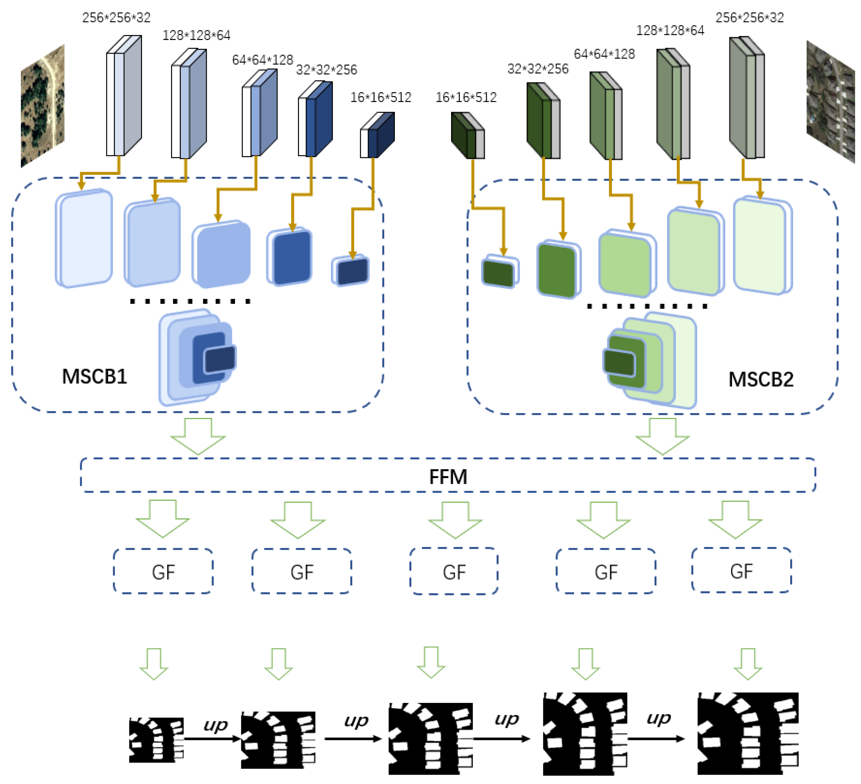
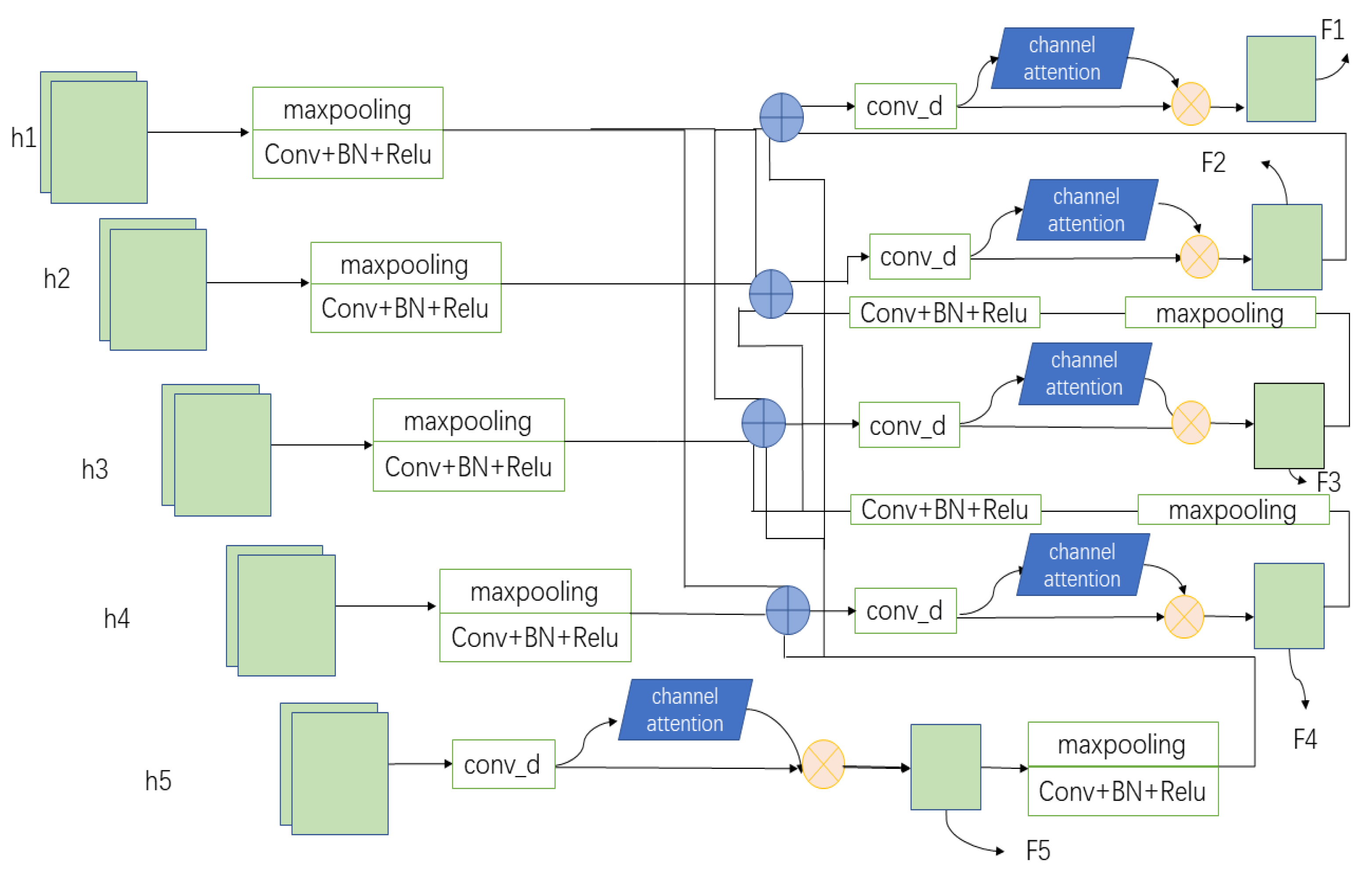
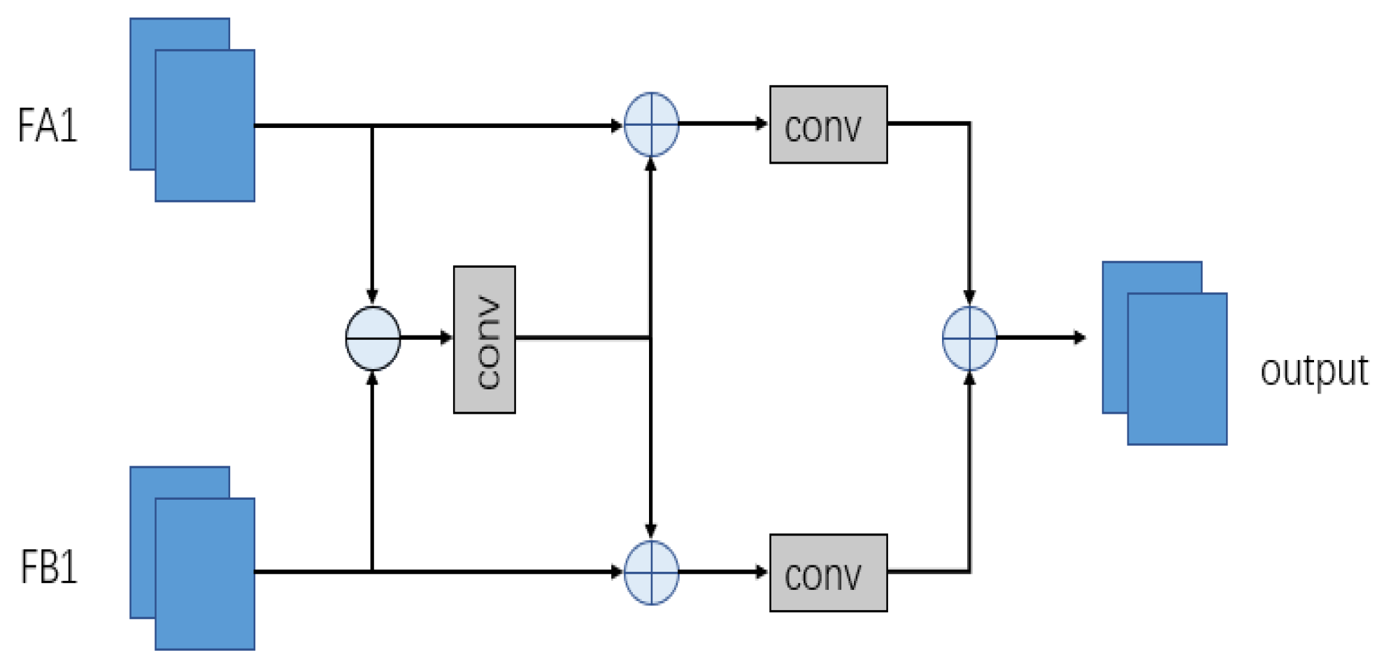
• In order to better extract comprehensive information and help the network to find regions of interest in images with large regional coverage, the muti-scale combination module (MSCB) and feature fusion module (FFM) are proposed. Since change detection data usually include change targets of different sizes, a multi-scale processing approach can be effective, bringing different perceptual fields and, thus, taking care of global and local feature information. As a necessary component of deep learning-based dual-temporal change detection, FFM fuses dual-temporal images and obtains the fused change results. These two modules can better serve for change detection.
• We use the GF, which can simulate the interaction between different spatial locations, navigating changes and non-changes at the pixel level in the same area. Therefore, our excellent combination of CNN and GF models can better improve the change detection model. Moreover, the global filter (GF) can avoid the huge computational complexity of the Transformer and use 2D Fourier transform and inverse 2D Fourier transform to process the image, which is an effective alternative to the Transformer. Through comparison and experiments with many baseline models, we verify the excellent ability of MFGFNet and confirm the effect of our network on three datasets, LEVIR-CD, SYSU, and CDD.

The remainder of this article is organized into four sections. Section 2 introduces some preliminary knowledge of traditional CNN-based methods and frequency domain learning, and describes our network designs in detail. Section 3 provides experimental evaluations. Section 4 concludes this article.

2. Materials and Methods

2.1. Related Work

2.1.1. Traditional CNN-Based Method

CNN has undergone many years of development since its emergence and has become the basic operation for deep learning to extract features. Daudt et al. [6] designed three fully connected convolutional neural networks for change detection, FC-EF, FC-Siam-conc, and FC-Siam-diff, respectively. Fang et al. [23] proposed SNUNet-CD, and they used U-net as the backbone network. Compared with fully convolutional networks, they used the channel attention module (CAM) in deep supervision and added the ensemble channel attention module (ECAM), which can extract features in remote sensing images and increase the performance of the model. Peng et al. [24] used a new method based on self-attention for optical remote sensing images and obtained a better result. Based on the previous work, Zhang et al. [25] designed IFN and proposed extracting the deep features of the images first, and then differential discrimination and fusion. In a classical work. Chen et al. [26] introduced Transformer into the network to obtain more contextual information and enhance the original pixel-level features. Their proposed model was better than the pure CNN model at that time. In this network, unlike most transformer-based networks, it is not too large in FLOPs and the parameter. Chen et al. [27] created EGDE-Net, which contains in its encoder an edge-guided Transformer block, embedded with an edge-aware module and a feature differential enhancement module. Together, these three elements provide very good change detection and meet the need for capturing more information. Song et al. [28] proposed a new network using the Transformer (DMATNet), which can incrementally update image information, focus on regions of interest to avoid the influence of irrelevant regions on change detection, continuously sample to leave useful information, and reduce the weight of useless information, and finally improve the accuracy of change detection.

To date, many excellent works based on deep learning for change detection continue to emerge, and the accuracy metrics of change detection continue to improve, bringing continuous innovation to the field [29,30,31,32,33,34,35,36,37,38].

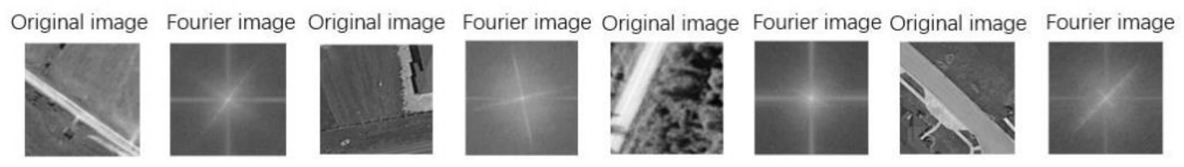
2.1.2. Frequency Domain Learning

In a typical deep learning network, the CNN is responsible for extracting image features, which belong to the spatial domain information. Figure 1 shows the spectrogram of some of the remote sensing images converted to 2D visualization in the frequency domain by the 2D Fourier transform. The spectrogram represents the distribution map of image gradients. A point on a spectrogram indicates the size of the gradient at a point of the graph in the spatial domain, and a large gradient means a high frequency. In recent years, there has been some research on the conversion of spatial domain information to the frequency domain for analysis, and the application effect has improved. Generally, there will be pre-processing in the frequency domain, transformed to the frequency domain with different Fourier change formulas. Moreover, the feature input in the frequency domain can be processed and applied to all CNN models in the spatial domain [39].

While architectures such as CNN and Transformer are widely popular in the field of computer vision, Rao et al. incorporated the traditional Fourier transform into the CNN-style and Transformer-style architectures and proposed the efficient and excellent GFNet. They demonstrated that the global filter layer is equivalent to a depth-wise global circular convolution filter of size H × W and is better at capturing the relationship between the frequency domains. There are also some deep learning networks based on frequency domain learning that are used in different areas. In the work by Zheng et al. [40], they use fast discrete CT to extract frequency domain features and achieve better results in object detection. Nurullah Sevim et al. [41] replaced the attention layer in the transformer with Fourier variation, achieving faster training, smaller memory, and eliminating the computational burden of the attention mechanism, which has been successfully applied to the field of NLP.

2.2. Framework Overview

Change detection can be understood as the segmentation of bitemporal remote sensing images according to the region of change. Our MFGFNet is a typical model that uses a combination of CNN and GF; it can fully extract changing ground objects by inputting bitemporal remote sensing images. As a Siamese network, MFGFNet has the same architecture in the first part. When we input two images, it can fully extract the global effective information and find the area of interest in the image covered by a large area. Moreover, our network adopts the idea of cascading semantic segmentation for feature refinement to better ensure the preservation of information at different scales. The specific structure of MFGFNet is fully demonstrated in Figure 2. After the image is input, it first goes through the convolution module, which includes convolution, batch normalization, and Relu. We add five groups of convolution modules for feature extraction, and then keep five groups of different sizes of maps for the next image processing. Next, the two sets of images go through MSCB, which combines images of different scales by upsampling, and then obtains a 64-channel image by convolution operation, which still gives five outputs (but all channels are 64). Furthermore, we obtain a multi-scale set of images with feature maps of sizes 256 × 256 × 32, 128 × 128 × 64, 64 × 64 × 128, 32 × 32 × 256, and 16 × 16 × 512. FFM is the module that plays the role of feature fusion in the overall network, comparing the differences between the different time phases and focusing on the parts that differ. Let the two bitemporal images be A, B; when MSCB1 outputs FA1, FA2, FA3, FA4, FA5, and MSCB2 outputs FB1, FB2, FB3, FB4, and FB5, FFM combines the FA1 and FB1 correspondences to find the difference between FA1 and FB1, and the difference is multiplied with the original input and then concatenates them both. Finally, the convolution to the channel is 64. Similarly, FA2 is combined with FB2, FA3 is processed together with FB3, etc. After processing by the FFM module, the 10 inputs are converted into 5 outputs after feature fusion, and these 5 outputs are fed to the GF for more information. Through these processes, five outputs of sizes 256 × 256, 128 × 128, 64 × 64, 32 × 32, and 16 × 16 are finally obtained; the number of channels is 64. Corresponding to different sizes, we will gradually upsample and convolve five groups of 256 × 256 × 2-sized images and multiply with the one after passing the channel attention. In our network, the binary cross-entropy loss is used as the loss function.

2.3. Multi-Scale Combination Module

In order to take into account the different receptive fields, a new multi-scale fusion method is proposed and used in our model (Figure 3). In Figure 3, there are 5 inputs and 5 outputs, and F5 is simply convolved through the inputs of 256 × 256 × 32 size to a channel of 64, then multiply it with the output through the channel attention. Figure 3 shows multiple maxpooling modules, where maxpooling does not simply mean a kernel_size and stride but represents different pooling effects on requirements, for example, when generating F3, F4, F5, and h1 and h2 by pooling to 64 × 64, at this time h3 cannot conduct the maxpooling operation. Taking F4 as an example, MSCM first resamples h1, h2, h3, and F5 as 32 × 32, then uses the resampled result to concatenate with h4 and convolve it, adjusting the number of channels to 64; finally, it concatenates it into a 32 × 32 × 320 image and adjusts the number of channels to 64 by conv_d to obtain F4, where conv_d includes the convolution operation, batch normalization, and Relu. The formulas are described as follows:

$$F_k{}^{\prime }=Conv\_d\left({\displaystyle \sum }_{i=1}^{k}MCBR \left(h_i\right)+{\displaystyle \sum }_{i=k+1}^5{F}_{k+1}\right)\left(k=1,2,3,4\right)$$

(1)

$$F_k=F_k^{\prime } \otimes \mathrm{CA}\left(F_k{}^{\prime }\right)$$

(2)

$$F_5=CA\left(Conv\_d\left(h_5\right)\right)+\mathrm{Conv}\_\mathrm{d}\left(h_5\right)$$

(3)

where MCBR represents the four operations of maxpooling, convolution, batch normalization, and Relu. It is important to note that maxpooling is not a fixed parameter value, but is adjusted according to different needs. ${\displaystyle \sum }$ and + represent the concatenated operation on the channel dimension. Conv_d is an operation that can reduce the channel to 64. CA means the channel attention model (CAM) [42]. $\otimes$ is an element-wise multiplication.

2.4. Feature Fusion Module

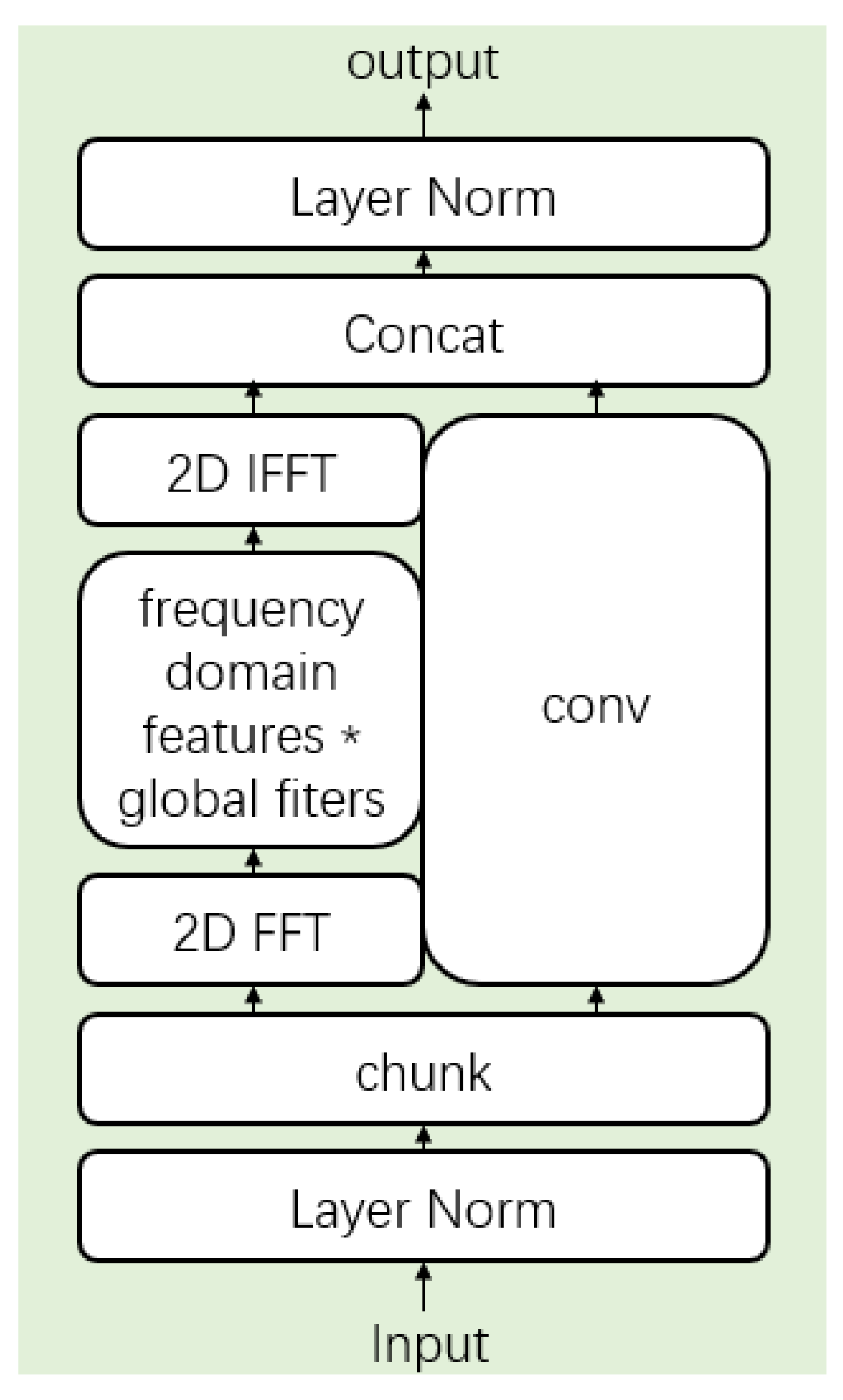
FFM is indispensable in the change detection model, which serves the function of detecting the differences in bitemporal images, fusing them into a new graph. The FFM fuses each corresponding two pairs into one; the structure of the FFM is shown in Figure 4 with two pairs as an example. FFM fuses two pairs of images together, an operation that is almost necessary for deep learning change detection.

When it is FFM’s turn to work, it will process FA1 and FB1 together. In the processing process, the difference between them will be calculated first, then they will pass through a 3 × 3 convolution and be added to the original input, respectively; finally, they will be convolved separately and then added to obtain the output. The formulas are described as follows:

$$De=Conv\left(\left|FA1-FB1\right|\right)$$

(4)

$$F{1}^{\prime }=Conv\left(Concat\left(FA1,De\right)\right)$$

(5)

$$F{2}^{\prime }=Conv\left(Concat\left(FB1,De\right)\right)$$

(6)

$$Output=Conv\left(Concat\left(F{1}^{\prime }, F{2}^{\prime }\right)\right)$$

(7)

where |·| means an absolution operation, $-$ is an element-wise subtraction operation. De denotes a result that is obtained by the $-$. F1${}^{\prime }$ represents the combination of FA1 and De. F2${}^{\prime }$ represents the combination of FB1 and De. The final output is convolved from F1 and F2. The formula is written by taking FA1 and FB1 as examples. See Figure 4 for the specific structure.

2.5. Global Filter

The specific details of the global filter are clearly shown in Figure 5. The core of the global filter uses the knowledge of the discrete Fourier transform (DFT). For a given image, the DFT as a whole is unique, so for the results obtained by the DFT operation, the original data can be recovered by inverse DFT (IDFT). As a method where both the input and output are discrete values, DFT is well suited for processing with computers. DFT can also expand the input to 2D. This 2D DFT can be regarded as the replacement of two 1D DFTs and provide computational efficiency; 2D DFT and 2D IDFT are used in GF to achieve the effect of capturing the frequency domain. Figure 6 shows the visualization of GFs.

In the GF, to better combine the different advantages of the spatial and frequency domains, we used half of the channels to perform frequency domain learning operations, mainly including 2D discrete Fourier transform to convert the input spatial features to the frequency domain, perform element-wise multiplication between the frequency domain features and the global filter, and 2D inverse Fourier transform to map the features back to the spatial domain. The other half uses 3 × 3 depth-wise convolution and then combines the two to obtain the result [43]. The mathematical formulas for the two-dimensional discrete Fourier transform and the inverse transform are as follows:

$$F\left(x,y\right)={\displaystyle \sum }_{x=0}^{M-1}{\displaystyle \sum }_{y=0}^{N-1}f\left(x,y\right)e^{-j2\pi \left(\frac{ux}{M}+\frac{vy}{N}\right)}$$

(8)

$$f\left(x,y\right)=\frac{1}{MN}{\displaystyle \sum }_{u=0}^{M-1}{\displaystyle \sum }_{v=0}^{N-1}F\left(u,v\right)e^{j2\pi }\left(\frac{ux}{M}+\frac{vy}{N}\right)$$

(9)

where Equation (8) represents the 2D discrete Fourier transform and Equation (9) represents the inverse 2D discrete Fourier transform. M and N are the length and width of the image, respectively. u and x range from 1 to M − 1; v and y range from 1 to N − 1.

3. Experiments and Results

3.1. Dataset

Since the introduction of deep learning for change detection, many change detection datasets have emerged such as AICD, HRSCD, Mts-WH, S2Looking, WHU Building, and change detection [4,44,45,46,47]. We used LEVIR [3], SYSU [4], and CDD [48].

3.1.1. LEVIR-CD Dataset

LEVIR-CD is a large-scale change detection dataset composed of Google Earth image block pairs extracted by Beihang University, where the image pairs are all 1024 × 1024 in size. We downloaded LEVIR-CD and cropped it to 256 × 256. When the image in the LEVIR-CD is cropped to 256 × 256 size, it contains 7120 pairs of bitemporal images for model training. At the same time, this dataset prepares 2048 pairs of bitemporal images for the test set, and the validation set includes 1024 pairs of bitemporal images, respectively.

3.1.2. SYSU Dataset

This dataset contains 20,000 pairs of 0.5 m aerial images, 256 × 256 in size, taken in Hong Kong between 2007 and 2014. The SYSU-CD dataset contains 12,000 pairs of bitemporal images for model training. Moreover, this dataset prepares 4000 pairs of bitemporal images for the test set, and the validation set concludes with 4000 pairs of bitemporal images. The SYSU dataset mainly includes the expansion of suburbs, new buildings in Hong Kong, road construction, vegetation changes, etc.

3.1.3. CDD Dataset

Among the various datasets for change detection, CDD is an excellent dataset. The CDD dataset has three types of remote sensing images: synthetic images with no relative movement of objects, synthetic images with little relative movement of objects, and real remote sensing images that change with the seasons. The spatial resolution of these images ranges from 3 cm to 1 m, and all images are 256 × 256. Our experiments use different change detection models to conduct multiple sets of comparative experiments on the CDD dataset. The CDD dataset contains 10,000 pairs of multitemporal images for model training. At the same time, this dataset prepares 3000 pairs of multitemporal images for the test set and validation set, respectively.

3.2. Implementation Details

We implemented the model in this paper using PyTorch and completed all experiments on four RTX 2080 Ti. We used the Adam optimizer and set β1 at 0.9, β2 at 0.999, the learning rate at 0.001, the batch size was adjusted to 16 in all training sets, and the weight decay was 0.01. In terms of the experiments on the LEVIR-CD, we set the learning rate to 0.001 and a total of 100 epochs were trained. For the SYSU dataset, the initial learning rate was 0.001 and a total of 80 epochs were trained. For the CDD change detection dataset, the initial learning rate was 0.0002 and a total of 100 epochs were trained. In the training process, the weight decay was 0.01, eps was 1 × 10⁻⁸, and the Kaiming initialization was used for all convolutional layers.

3.3. Evaluation Criteria

Considering the evaluation indicators commonly used in change detection, we used the three most typical metrics to evaluate the experimental results, they are precision, recall, F1-score, OA, and IoU. The above five indicators can be represented by TP, FP, FN, and TN, where TP represents true positive, TN means true negative, FP means false positive, and FN means false negative. These operations can be represented as follows:

$$Precision=\frac{TP}{TP+FP}$$

(10)

$$Recall=\frac{TP}{TP+FN}$$

(11)

$$F1=\frac{2\ast Precision\ast Recall}{Precision+Recall}$$

(12)

$$OA=\frac{TP+TN}{TP+FP+FN+TN}$$

(13)

$$IoU=\frac{TP}{TP+FP+FN}$$

(14)

3.4. Comparison and Analysis

In testing the three datasets (LEVIR-CD, SYSU, and DSIFN), we used six very good change detection algorithms: FC-conc, FC-diff, IFN, DDCNN, SNUNet, and BIT. The obtained results show that our deep learning model achieves better results in all three datasets and gives more excellent results compared to the other outstanding algorithms.

3.4.1. Results for LEVIR-CD

In Figure 7, the results of a partial visualization of the LEVIR-CD dataset are shown and

Table 1. The comparison results on the LEVIR-CD dataset.

Method	Pre	Rec	F1	OA	IOU
FC-Conc	0.8063	0.7677	0.7865	0.9787	0.6482
FC-Diff	0.8222	0.6929	0.7520	0.9767	0.6026
IFN	0.9154	0.6128	0.7354	0.9775	0.5816
DDCNN	0.8542	0.8031	0.8279	0.9830	0.7063
SNUNet	0.9040	0.8742	0.8889	0.9888	0.8000
BIT	0.9130	0.8651	0.8884	0.9889	0.7992
Ours	0.9155	0.9014	0.9084	0.9907	0.8322

details the accuracy metrics obtained by the different algorithms. A total of four pairs of bitemporal images were selected, including two pairs of large building change images and two pairs of dense building cluster images. By comparing the results, we can see that the MFGFNet visualization basically has no red and green parts, which is more advantageous than the other. In the LEVIR-CD data, most of the models are adequate for the change detection of large buildings, with only a few being less effective. Among them, our models have the best ability to capture large buildings. All models perform well for changes in dense buildings, indicating that these models are sensitive to dense and small targets. MFGFNet shows excellent ability in LEVIR-CD, it is especially good at detecting small feature changes and achieves the best results in all metrics except precision, and the overall effect is the best among all comparison models.

In Table 1, we can see that the precision algorithms FC-conc and FC-diff are not effective, where the precision of FC-diff is 0.8222, which is better than the precision of FC-conc; however, the other four metrics are better for FC-conc. The precision of IFN reaches 0.9154, which is the second highest of the algorithms used in the paper. However, the other metrics of IFN are not as good as FC-diff and FC-conc, and the overall performance is the worst. The accuracy of DDCNN is more ordinary, and the result is better than FC-diff and FC-conc. For both models, SNUNet and BIT, the accuracy on the LEVIR-CD dataset is outstanding; F1, OA, and IOU are very close in both models, with slightly higher precision for BIT and slightly higher recall for SNUNet.

3.4.2. Results for SYSU

Figure 8 shows the qualitative analysis of change detection in the SYSU dataset, with a total of four pairs of bitemporal images selected, including large buildings and chains.

In the SYSU results presentation, we see that FC-conc and FC-diff work better than expected, probably because these two models are more suitable for this dataset. Our network shows very good results in the four sets of demonstrations, both in building and ship changes, which is due to the fact that our network can capture the edges of the changes better with few error detections.

In the

Table 2. The comparison results on the SYSU dataset.

Method	Pre	Rec	F1	OA	IOU
FC-Conc	0.7300	0.7680	0.7485	0.8783	0.5981
FC-Diff	0.8769	0.5133	0.6476	0.8682	0.4788
IFN	0.8777	0.5697	0.6909	0.8798	0.5278
DDCNN	0.7209	0.8230	0.7686	0.8831	0.6241
SNUNet	0.7865	0.7647	0.7754	0.8955	0.6333
BIT	0.7874	0.7653	0.7762	0.8959	0.6343
Ours	0.8232	0.7936	0.8081	0.9111	0.6780

, the effect of FC-Conc is significantly better than that of FC-diff. The IoU of FC-conc reaches 0.5981; however, the IoU of FC-diff is only 0.4788, which is a big difference between them. IFN is worse than FC-conc, but better than FC-diff, with an IoU of 0.5278 in the result, where precision, as in the previous LEVIR-CD dataset, reaches 0.8777, the highest of all algorithms. Both DDCNN and SNUNet obtained good results in this dataset. Overall, SNUNet is slightly better, but DDCNN achieves the best accuracy recall in SYSU, up to 0.8230. BIT did not achieve the desired results in the SYSU dataset, only better than IFN and FC-diff, and all accuracy metrics were unsatisfactory. Our model exhibits excellent performance across all metrics, with the best values achieved in F1, OA, and IoU, but due to the large number of targets in this dataset, not all aspects work very well.

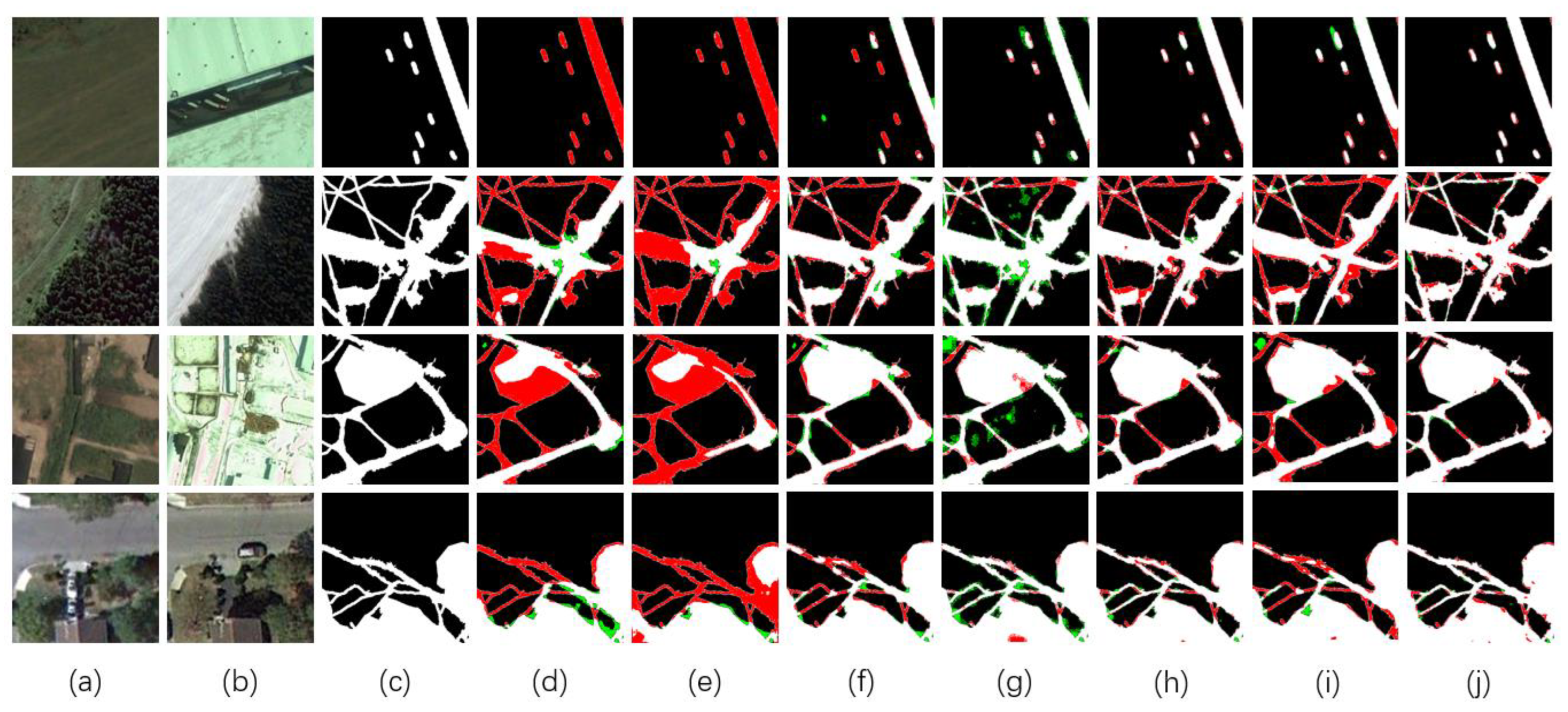
3.4.3. Results for CDD

The CDD contains real remote sensing images that change with the seasons. Our network achieved the best results and selected four different pairs of images to show the visual effects of various networks. In Figure 9, our network is well adapted to the effects of seasonal changes, and we can avoid missing and incorrect detections better than other algorithms because our model possesses a better ability to achieve change detection. For the road changes, we can see that FC-diff and FC-Conc are almost unrecognizable, and DDCNN, SNUNet, and BIT have some error detection and omission detection, while our model has only minor omission detection. For complex seasonal changes, FC-diff and FC-conc are equally ineffective, DDCNN has some error detection, and the change maps obtained by our model in comparison with SNUNet and BIT are the closest to the real seasonal change results.

In the CDD data, we trained 100 epochs for each comparison network to obtain

Table 3. The comparison results on the CDD dataset.

Method	Pre	Rec	F1	OA	IOU
FC-Conc	0.8668	0.6004	0.7094	0.9419	0.5497
FC-Diff	0.8920	0.4501	0.5983	0.9286	0.4269
IFN	0.9108	0.8889	0.8997	0.9766	0.8177
DDCNN	0.9008	0.8297	0.8638	0.9662	0.7602
SNUNet	0.9543	0.9420	0.9481	0.9878	0.9014
BIT	0.9512	0.8673	0.9073	0.9791	0.8303
Ours	0.9564	0.9494	0.9529	0.9889	0.9101

. After a comparison, our MFGFNet obtained good results for SOTA, with an F1 of 0.9529, which is much higher than the other comparison networks. As the training and test sets in the CDD dataset may be highly similar, the model did not converge when we trained to 100 epochs. If we continue to train for 150 or 200 epochs or even more, our model F1 might be able to reach 0.97 or higher. Figure 9 shows the qualitative analysis of the change detection on the CDD dataset, with a total of four pairs of diachronic images selected, including different seasonal changes. In the visualization plots, we can see that FC-diff and FC-conc are very poor, with large areas of red and green in the plots, whereas our MFGFNet plots obtained by visualization are significantly less cluttered and better (Figure 9).

3.5. Ablation Study

To test the three components of our model (FFM, MSCB, GF), we conducted four sets of experiments on LEVIR-CD, using only FFM, FFM + MSCB, FFM + GF, and FFM + MSCB + GF. All four cases were first extracted by the convolutional neural network with features of different scales. The specific results can be viewed in

Table 4. The quantitative results of the ablation study on the LEVIR-CD dataset.

FFM	MSCB	GF	Pre	Rec	F1	OA	IOU
√	×	×	0.8917	0.8512	0.8710	0.9871	0.7715
√	√	×	0.9003	0.8878	0.8940	0.9892	0.8083
√	×	√	0.9131	0.8773	0.8949	0.9895	0.8098
√	√	√	0.9155	0.9014	0.9084	0.9907	0.8322

. Through multi-pair experiments, we see that when only FFM is used (i.e., feature extraction followed by difference and convolution), the results obtained show that the task of change detection can be basically accomplished, and the results are still better than the classical FC-diff, FC-conc. The data in the table show that when only FFM is used, the results are already better than many good algorithms.

In addition to the case where only FFM was used, we designed two comparative experiments, FFM + MSCB and FFM + GF. The experimental results show that the two effects are similar, better than using only FFM and worse than FFM + MSCB + GF. The IoU of FFM + MSCB reaches 0.8083 and that of FFM + GF reaches 0.8098. Through these two sets of experiments, it is shown that MSCB and GF modules play a very important role in MFGFNet, bringing great power. At the same time, the results of FFM + GF also show that learning in the frequency domain can play a certain effect in deep learning.

The best results were achieved in LEVIR-CD when all modules of MFGFNet were working. FFM + MSCB + GF outperformed the other three groups of experiments and its excellent results demonstrate the validity of our model. In this case, it reached the IoU of 0.8322, which is worse than the other three groups with differences of 0.0224, 0.0239, and 0.0428, respectively. In conclusion, all modules of MFGFNet show excellent capabilities.

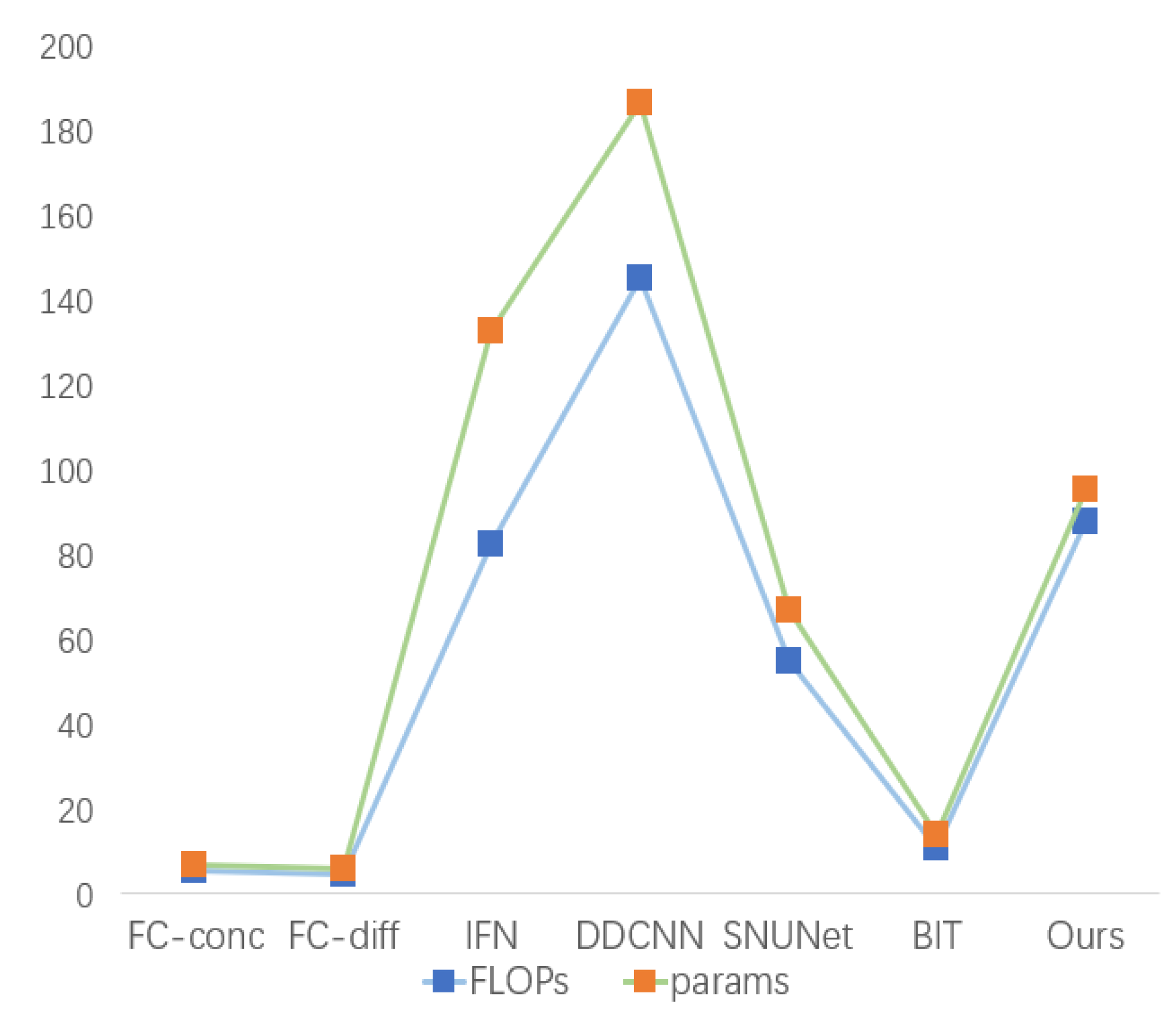
3.6. Parameter Comparison

In this paper the FLOPs and params were calculated for different networks at work; Figure 10 illustrates the two parameters in a line graph for different networks. As can be seen from the graph, our FLOPs and params are neither the highest nor the lowest and do not compare favorably with such algorithms as FC-conc and FC-diff, but this cost can be neglected for accuracy improvement. At the same time, our network reduces these two parameters compared to other large models, such as DDCNN, bringing strength to the overall performance.

4. Conclusions

In this paper, we propose a CNN-based network for remote sensing change detection (MFGFNet) using frequency domain learning enhancement. Our network first uses the Siamese CNN structure to extract features in the images. In order to take into account the change information at different scales, we fused the image features continuously upwards and combined them with a channel attention mechanism to obtain a new output. In this case, each pair of images was fused and then passed through the global filter, which captured the frequency parts of the image to sharpen the image and preserve more edge information, thus improving accuracy. Our experiments demonstrate the excellent performance of MFGFNet, which compares well with other state-of-the-art networks.

In the future, we will improve the weakly supervised and unsupervised change detection networks to better meet the engineering needs of the real-world applications of change detection where the training set and test data do not match and the label quality is poor. Moreover, due to the lack of change feature classes in practical applications of binary change detection (BCD), semantic change detection (SCD) is gradually becoming a mainstream research direction. Transforming dichotomous change detection into semantic change detection can better serve important issues (such as land use). Thus, we hope to improve MFGFNet to make it a network to solve the SCD problem.

References

1. Lu, D.; Mausel, P.; Brondízio, E.; Moran, E. Change detection techniques. Int. J. Remote Sens. 2004, 25, 2365–2401. [Google Scholar] [CrossRef]
2. Hussain, M.; Chen, D.; Cheng, A.; Wei, H.; Stanley, D. Change detection from remotely sensed images: From pixel-based to object-based approaches. ISPRS J. Photogramm. Remote Sens. 1998, 80, 91–106. [Google Scholar] [CrossRef]
3. Chen, H.; Shi, Z. A spatial-temporal attention-based method and a new dataset for remote sensing image change detection. Remote Sens. 2020, 12, 1662. [Google Scholar] [CrossRef]
4. Ji, S.; Wei, S.; Lu, M. Fully convolutional networks for multisource building extraction from an open aerial and satellite imagery data set. IEEE Trans. Geosci. Remote Sens. 2019, 57, 574–586. [Google Scholar] [CrossRef]
5. Peng, D.; Zhang, Y.; Guan, H. End-to-end change detection for high resolution satellite images using improved UNet++. Remote Sens. 2019, 11, 1382. [Google Scholar] [CrossRef] [Green Version]
6. Daudt, R.C.; Le Saux, B.; Boulch, A. Fully convolutional Siamese networks for change detection. In Proceedings of the 25th IEEE International Conference on Image Processing (ICIP), Athens, Greece, 7–10 October 2018; pp. 4063–4067. [Google Scholar] [CrossRef] [Green Version]
7. Yu, X.; Fan, J.; Chen, J.; Zhang, P.; Zhou, Y.; Han, L. NestNet: A multiscale convolutional neural network for remote sensing image change detection. Int. J. Remote Sens. 2021, 42, 4898–4921. [Google Scholar] [CrossRef]
8. Shi, Q.; Liu, M.; Li, S.; Liu, X.; Wang, F.; Zhang, L. A deeply supervised attention metric-based network and an open aerial image dataset for remote sensing change detection. IEEE Trans. Geosci. Remote Sens. 2021, 60, 5604816. [Google Scholar] [CrossRef]
9. Chen, J.; Yuan, Z.; Peng, J.; Chen, L.; Huang, H.; Zhu, J.; Liu, Y.; Li, H. DASNet: Dual attentive fully convolutional Siamese networks for change detection in high-resolution satellite images. IEEE J. Sel. Top. Appl. Earth Observ. Remote Sens. 2021, 14, 1194–1206. [Google Scholar] [CrossRef]
10. Li, Z.; Yan, C.; Sun, Y.; Xin, Q. A Densely Attentive Refinement Network for Change Detection Based on Very-High-Resolution Bitemporal Remote Sensing Images. IEEE Trans. Geosci. Remote Sens. 2022, 60, 1–18. [Google Scholar] [CrossRef]
11. Lei, T.; Wang, J.; Ning, H.; Wang, X.; Xue, D.; Wang, Q.; Nandi, A.K. Difference Enhancement and Spatial–Spectral Nonlocal Network for Change Detection in VHR Remote Sensing Images. IEEE Trans. Geosci. Remote Sens. 2022, 60, 1–13. [Google Scholar] [CrossRef]
12. Basavaraju, K.S.; Sravya, N.; Lal, S.; Nalini, J.; Reddy, C.S.; Dell’Acqua, F. UCDNet: A Deep Learning Model for Urban Change Detection From Bi-Temporal Multispectral Sentinel-2 Satellite Images. IEEE Trans. Geosci. Remote Sens. 2022, 60, 1–10. [Google Scholar] [CrossRef]
13. Yang, Y.; Gu, H.; Han, Y.; Li, H. An End-to-End Deep Learning Change Detection Framework for Remote Sensing Images. In Proceedings of the IGARSS 2020—2020 IEEE International Geoscience and Remote Sensing Symposium, Waikoloa, HI, USA, 26 September–2 October 2020. [Google Scholar]
14. Zhu, X.; Su, W.; Lu, L.; Li, B.; Wang, X.; Dai, J. Deformable DETR: Deformable transformers for end-to-end object detection. arXiv 2020, arXiv:2010.04159. [Google Scholar]
15. Zheng, S.; Lu, J.; Zhao, H.; Zhu, X.; Luo, Z.; Wang, Y.; Fu, Y.; Feng, J.; Xiang, T.; Torr, P.H.S.; et al. Rethinking semantic segmentation from a sequence-to-sequence perspective with transformers. In Proceedings of the IEEE/CVF Conference on Computer Vision and Pattern Recognition (CVPR), Nashville, TN, USA, 20–25 June 2021; pp. 6881–6890. [Google Scholar]
16. Dosovitskiy, A.; Beyer, L.; Kolesnikov, A.; Weissenborn, D.; Zhai, X.; Unterthiner, T.; Dehghani, M.; Minderer, M.; Heigold, G.; Gelly, S.; et al. An image is worth 16×16 words: Transformers for image recognition at scale. arXiv 2020, arXiv:2010.11929. [Google Scholar]
17. Pang, L.; Sun, J.; Chi, Y.; Yang, Y.; Zhang, F.; Zhang, L. CD-TransUNet: A Hybrid Transformer Network for the Change Detection of Urban Buildings Using L-Band SAR Images. Sustainability 2022, 14, 9847. [Google Scholar] [CrossRef]
18. Li, Q.; Zhong, R.; Du, X.; Du, Y. TransUNetCD: A Hybrid Transformer Network for Change Detection in Optical Remote-Sensing Images. IEEE Trans. Geosci. Remote Sens. 2022, 60, 1–19. [Google Scholar] [CrossRef]
19. Wang, W.; Tan, X.; Zhang, P.; Wang, X. A CBAM Based Multiscale Transformer Fusion Approach for Remote Sensing Image Change Detection. IEEE J. Sel. Top. Appl. Earth Observ. Remote Sens. 2022, 15, 6817–6825. [Google Scholar] [CrossRef]
20. Liu, Z.; Lin, Y.; Cao, Y.; Hu, H.; Wei, Y.; Zhang, Z.; Lin, S.; Guo, B. Swin transformer: Hierarchical vision transformer using shifted Windows. arXiv 2021, arXiv:2103.14030. [Google Scholar]
21. Zhang, C.; Wang, L.; Cheng, S.; Li, Y. SwinSUNet: Pure Transformer Network for Remote Sensing Image Change Detection. IEEE Trans. Geosci. Remote Sens. 2022, 60, 1–13. [Google Scholar] [CrossRef]
22. Rao, Y.; Zhao, W.; Zhu, Z.; Lu, J.; Zhou, J. Global filter networks for image classification. Adv. Neural Inf. Process. Syst. 2021, 34, 980–993. [Google Scholar]
23. Fang, S.; Li, K.; Shao, J.; Li, Z. SNUNet-CD: A densely connected Siamese network for change detection of VHR images. IEEE Geosci. Remote Sens. Lett. 2022, 19, 1–5. [Google Scholar] [CrossRef]
24. Peng, X.; Zhong, R.; Li, Z.; Li, Q. Optical remote sensing image change detection based on attention mechanism and image difference. IEEE Trans. Geosci. Remote Sens. 2021, 59, 7296–7307. [Google Scholar] [CrossRef]
25. Zhang, C.; Yue, P.; Tapete, D.; Jiang, L.; Shangguan, B.; Huang, L.; Liu, G. A deeply supervised image fusion network for change detection in high resolution bi-temporal remote sensing images. ISPRS J. Photogramm. Remote Sens. 2020, 166, 183–200. [Google Scholar] [CrossRef]
26. Chen, H.; Qi, Z.; Shi, Z. Remote sensing image change detection with transformers. IEEE Trans. Geosci. Remote Sens. 2021, 60, 1–14. [Google Scholar] [CrossRef]
27. Chen, Z.; Zhou, Y.; Wang, B.; Xu, X.; He, N.; Jin, S.; Jin, S. EGDE-Net: A building change detection method for high-resolution remote sensing imagery based on edge guidance and differential enhancement. ISPRS J. Photogram. Remote Sens. 2022, 191, 203–222. [Google Scholar] [CrossRef]
28. Song, X.; Hua, Z.; Li, J. Remote Sensing Image Change Detection Transformer Network Based on Dual-Feature Mixed Attention. IEEE Trans. Geosci. Remote Sens. 2022, 60, 1–16. [Google Scholar] [CrossRef]
29. Khusni, U.; Dewangkoro, H.I.; Arymurthy, A.M. Urban area change detection with combining CNN and RNN from Sentinel-2 multispectral remote sensing data. In Proceedings of the International Conference on Computer and Informatics Engineering (IC2IE), Depok, Indonesia, 15–16 September 2020; pp. 171–175. [Google Scholar]
30. Papadomanolaki, M.; Verma, S.; Vakalopoulou, M.; Gupta, S.; Karantzalos, K. Detecting urban changes with recurrent neural networks from multitemporal Sentinel-2 data. In Proceedings of the 2019 IEEE International Geoscience and Remote Sensing Symposium(IGARSS), Yokohama, Japan, 28 July–2 August 2019; pp. 214–217. [Google Scholar]
31. Lei, T.; Zhang, Y.; Lv, Z.; Li, S.; Liu, S.; Nandi, A.K. Landslide inventory mapping from bitemporal images using deep convolutional neural networks. IEEE Geosci. Remote Sens. Lett. 2019, 16, 982–986. [Google Scholar] [CrossRef]
32. Daudt, R.C.; Le Saux, B.; Boulch, A.; Gousseau, Y. Urban change detection for multispectral earth observation using convolutional neural networks. In Proceedings of the 2018 IEEE International Geoscience and Remote Sensing Symposium (IGARSS), Valencia, Spain, 22–27 July 2018; pp. 2115–2118. [Google Scholar]
33. Yang, X.; Hu, L.; Zhang, Y.; Li, Y. MRA-SNet: Siamese networks of multiscale residual and attention for change detection in high resolution remote sensing images. Remote Sens. 2021, 13, 4528. [Google Scholar] [CrossRef]
34. Cheng, G.; Wang, G.; Han, J. ISNet: Towards Improving Separability for Remote Sensing Image Change Detection. IEEE Trans. Geosci. Remote Sens. 2022, 60, 1–11. [Google Scholar] [CrossRef]
35. Ding, L.; Guo, H.; Liu, S.; Mou, L.; Zhang, J.; Bruzzone, L. Bi-Temporal Semantic Reasoning for the Semantic Change Detection in HR Remote Sensing Images. IEEE Trans. Geosci. Remote Sens. 2022, 60, 1–14. [Google Scholar] [CrossRef]
36. Xu, J.; Luo, C.; Chen, X.; Wei, S.; Luo, Y. Remote sensing change detection based on multidirectional adaptive feature fusion and perceptual similarity. Remote Sens. 2021, 13, 3053. [Google Scholar] [CrossRef]
37. Bai, B.; Fu, W.; Lu, T.; Li, S. Edge-Guided Recurrent Convolutional Neural Network for Multitemporal Remote Sensing Image Building Change Detection. IEEE Trans. Geosci. Remote Sens. 2022, 60, 1–13. [Google Scholar] [CrossRef]
38. Lei, T.; Xue, D.; Ning, H.; Yang, S.; Lv, Z.; Nandi, A.K. Local and Global Feature Learning With Kernel Scale-Adaptive Attention Network for VHR Remote Sensing Change Detection. IEEE J. Sel. Top. Appl. Earth Observ. Remote Sens. 2022, 15, 7308–7322. [Google Scholar] [CrossRef]
39. Xu, K.; Qin, M.; Sun, F.; Wang, Y.; Chen, Y.-K.; Ren, F. Learning in the Frequency Domain. In Proceedings of the 2020 IEEE/CVF Conference on Computer Vision and Pattern Recognition (CVPR), Seattle, WA, USA, 13–19 June 2020; pp. 1737–1746. [Google Scholar] [CrossRef]
40. Zheng, S.; Wu, Z.; Xu, Y.; Wei, Z.; Plaza, A. Learning Orientation Information From Frequency-Domain for Oriented Object Detection in Remote Sensing Images. IEEE Trans. Geosci. Remote Sens. 2022, 60, 1–12. [Google Scholar] [CrossRef]
41. Sevim, N.; Ozan Özyedek, E.; Şahinuç, F.; Koç, A. Fast-FNet: Accelerating Transformer Encoder Models via Efficient Fourier Layers. arXiv 2022, arXiv:2209.12816. [Google Scholar]
42. Hu, J.; Shen, L.; Albanie, S.; Sun, G.; Wu, E. Squeeze-and-excitation networks. IEEE Trans. Pattern Anal. Mach. Intell. 2020, 42, 2011–2023. [Google Scholar] [CrossRef] [Green Version]
43. Rao, Y.; Zhao, W.; Tang, Y.; Zhou, J.; Lim, S.; Lu, J. Hornet: Efficient high-order spatial interactions with recursive gated convolutions. arXiv 2022, arXiv:2207.14284. [Google Scholar]
44. Bourdis, N.; Marraud, D.; Sahbi, H. Constrained optical flow for aerial image change detection. In Proceedings of the 2011 IEEE International Geoscience and Remote Sensing Symposium, Vancouver, BC, Canada, 24–29 July 2011; pp. 4176–4179. [Google Scholar] [CrossRef] [Green Version]
45. Daudt, R.C.; Le Saux, B.; Boulch, A.; Gousseau, Y. Multitask learning for large-scale semantic change detection. Comput. Vis. Image Underst. 2019, 187, 102783. [Google Scholar] [CrossRef] [Green Version]
46. Wu, C.; Zhang, L.; Du, B. Kernel Slow Feature Analysis for Scene Change Detection. IEEE Trans. Geosci. Remote Sens. 2017, 55, 2367–2384. [Google Scholar] [CrossRef]
47. Shen, L.; Lu, Y.; Chen, H.; Wei, H.; Xie, D.; Yue, J.; Chen, R.; Lv, S.; Jiang, B. S2Looking: A satellite side-Looking dataset for building change detection. Remote Sens. 2021, 13, 5094. [Google Scholar] [CrossRef]
48. Lebedev, M.A.; Vizilter, Y.V.; Vygolov, O.V.; Knyaz, V.A.; Rubis, A.Y. Change detection in remote sensing images using conditional adversarial networks. ISPRS-Int. Arch. Photogramm. Remote Sens. Spat. Inf. Sci. 2018, 2, 565–571. [Google Scholar] [CrossRef] [Green Version]
Figure 1. Part of the remote sensing images and their transformation into a spectrogram of the two-dimensional visualization in the frequency domain.
Remotesensing 15 01682 g001
Figure 2. Structure of the MFGFNet.
Remotesensing 15 01682 g002
Figure 3. Structure of the MSCB.
Remotesensing 15 01682 g003
Figure 4. Structure of FFM.
Remotesensing 15 01682 g004
Figure 5. Global filter. The * in the figure represents an element-wise multiplication between frequency-domain features and learnable global filters.
Remotesensing 15 01682 g005
Figure 6. Visualization of the global filters. A visualization of the 5 global filters of MFGFNet is included in Figure 6.
Remotesensing 15 01682 g006
Figure 7. Visualization results of different methods for LEVIR-CD datasets. (a) T1 images. (b) T2 images. (c) Ground truth. (d) FC-Conc. (e) FC-Diff. (f) IFN. (g) DDCNN. (h) SNUNet. (i) BIT. (j) Ours. In the figure, white, black, red, and green represent TP, TN, FN, and FP, respectively.
Remotesensing 15 01682 g007
Figure 8. Visualization results of different methods for SYSU datasets. (a) T1 images. (b) T2 images. (c) Ground truth. (d) FC-Conc. (e) FC-Diff. (f) IFN. (g) DDCNN. (h) SNUNet. (i) BIT. (j) Ours. In the figure, white, black, red, and green represent TP, TN, FN, and FP, respectively.
Remotesensing 15 01682 g008
Figure 9. Visualization results of different methods for CDD datasets. (a) T1 images. (b) T2 images. (c) Ground truth. (d) FC-Conc. (e) FC-Diff. (f) IFN. (g) DDCNN. (h) SNUNet. (i) BIT. (j) Ours. In the figure, white, black, red, and green represent TP, TN, FN, and FP, respectively.
Remotesensing 15 01682 g009
Figure 10. FLOPs and params.
Remotesensing 15 01682 g010