Comparing Water Indices for Landsat Data for Automated Surface Water Body Extraction under Complex Ground Background: A Case Study in Jilin Province

Abstract

Derived from Landsat imagery and capable of enhancing the contrast between surface water bodies and the background, water indices are widely used in surface water body extraction. Whether one index and its optimal threshold can maintain the best all year round is a question. At present, however, little research has considered the effect of time or conducted experiments with data from different months. To identify the best index for surface water body extraction, two regions in Jilin Province were selected for the case study and a comprehensive comparative analysis considering the imagery acquisition time was conducted. Ten water indices were selected and calculated based on the 30 m spatial resolution Landsat TM/OLI imagery acquired in 1999 and 2001 and 2019 and 2021 from May to October. The indices included the Modified Normalized Difference Water Index (NDWI3 and MNDWI), Automated Water Extraction Index (AWEI) for images with and without shadow, Multi-Band Water Index (MBWI), New Water Index (NWI), Water Ratio Index (WRI), Sentinel-2 Water Index (SWI) originally calculated based on the Sentinel-2 imagery, New Comprehensive Water Index (NCIWI), Index of Water Surfaces (IWS), and Enhanced Water Index (EWI). The OTSU algorism was adopted to adaptively determine the optimal segmentation threshold for each index and the indices were compared in terms of inter-class separability, threshold sensitivity, optimal threshold robustness, and water extraction accuracy. The result showed that NWI and EWI performed the best in different months and years, with the best water enhancement effect that could suppress background information, especially for the water-related land use types and cloud pollution. Their optimal segmentation thresholds throughout the study period were more stable than others, with the ranges of −0.342 to −0.038 and −0.539 to −0.223, respectively. Based on the optimal thresholds, they achieved overall accuracies of 0.952 to 0.981 and 0.964 to 0.981, commission errors of 0 to 28.2% and 0 to 7.7%, and omission errors of 0 to 15% and 0 to 8%, with a kappa coefficient above 0.8 indicating good extraction results. The results demonstrated the effectiveness of NWI and EWI combined with the OTSU algorithm in better monitoring surface water during different water periods and offering reliable results. Even though this study only focuses on the lakes within two regions, the indices have the potential for accurately monitoring the surface water over other regions.

1. Introduction

1.1. Background

Inland surface water bodies, such as rivers, lakes, reservoirs, and glaciers, are important components of the global water cycle and play an irreplaceable role in the global ecosystem and climate system [1]. As the direct source of fresh water in human life, surface water plays a vital role in industrial manufacturing, sustainable economic development, food production, and transportation [2,3]. However, in the context of global changes, water-related issues such as water shortage, floods, and water pollution have emerged in different parts of the world, posing serious challenges to water resources security [4,5]. According to the 2020 World Water Development Report, water security and climate change will be the persistent and profound global crises of the coming decades [6]. Therefore, identifying surface water bodies accurately and efficiently to monitor their spatial and temporal dynamics is crucial for understanding hydrological processes and sustainable management and the utilization of water resources [7]. Inland surface water bodies, especially seasonal rivers and lakes, have certain dynamic changes in water level and extent in different periods of the year, which can be better captured based on monthly monitoring [8].

Traditional surface water monitoring methods mainly rely on manual surveys in the field or are based on established gauge stations. Even though the accuracy of the acquired data is high, it is time-consuming work with low efficiency. In addition, many water bodies are in remote and rugged places, and only data from limited points at incomplete time series can be obtained due to the limitations of economic and terrain factors [2]. Recently, the development of remote sensing has provided a way to monitor water bodies widely spread over vast regions across long periods [9]. Nowadays, various remotely sensed data sets, such as optical multispectral images and synthetic aperture radar (SAR) images, are adopted to identify inland surface water, and valuable results have been achieved [10,11]. The complex data preprocessing, high costs, and short time spans of SAR data limited their applications in research on large regional scales for long periods [12]. At present, optical multispectral imageries obtained by MODIS, Landsat, and Sentinel-2 satellites are still the most commonly used data sources for water extraction. Considering the spatial resolution, revisit time, price, signal-to-noise ratio, and time span, Landsat imagery is one of the most widely applied and promising sources of data with the best performance.

Numerous techniques and algorithms have been developed to extract water based on multispectral imagery, among which the multiple-band spectral water index methods are the most popular as they are simple, efficient, and reproducible, especially for long-term and large-scale analyses. Water indices are often based on surface reflectance in the range from visible bands to short-wave infrared bands [13]. By enhancing the reflectance difference between water and non-water types, the indices can be used to extract water with optimal segmentation threshold values [14]. When extracting water bodies in a large region, the land background, the atmospheric condition and the water quality may be complex and affect the performance of this method. At present, scholars have conducted extensive research to detect water bodies based on water indices with different scenes, multispectral data sources, and spatial resolutions, to try to find a way to overcome this problem. The efforts have mainly been made with regard to the two key processes in the application of this method. One is the construction and selection of water index, and the other is the determination of the optimal segmentation thresholds.

1.2. Related Works

1.2.1. Construction and Selection of Water Index

Mcfeetersl developed the Normalized Difference Water Index (NDWI) based on the green band and the near-infrared (NIR) band of Landsat TM [15]. NDWI can effectively detect water in areas with high vegetation coverage, but water bodies are easily confused with construction sites in residential areas. Xu replaced the NIR band with the short-wave infrared (SWIR) band of Landsat TM to establish the Modified Normalized Difference Water Index (MNDWI), which made up for the limitations of NDWI and revealed the subtle characteristics of water and the distribution of suspended sediments, making it easier to distinguish shadows in water [16]. However, confusion between water bodies and the shadows of mountains and buildings remains. Additionally, optical images may also be contaminated by clouds and shadows, and the background in some regions is complex. Scholars have developed various indices to avoid these effects on the water extraction practice [14]. Only using NDWI or MNDWI may fail to distinguish the semidry water in semi-arid regions. Yan et al. introduced the Enhanced Water Index (EWI) to increase the difference between semi-dry rivers and the soil or residential areas, thus improving the water extraction accuracy [17]. The New Water Index (NWI) [18], a new Landsat Water Index proposed in 2015 (WI2015) [19], the Index of Water Surfaces (IWS) [20], and the Water Ratio Index (WRI) [21] were developed to suppress detailed information from the background and to enhance the water signal. Wang et al. established a robust Multi-Band Water Index (MBWI), which maintained a high water extraction accuracy in complex backgrounds with environmental noises [22].

In addition to adopting a single water index, some scholars also combined multiple water indices into a vector to extract water bodies. Feyisa et al. introduced the Automated Water Extraction Index (AWEI) consisting of two indices—AWEIsh and AWEInsh—to improve the water extraction accuracy in areas with dark surfaces and shadows [23]. Li et al. established a background difference water index (BDWI) vector consisting of three parts to avoid the impact of shadows in areas with complex backgrounds. After applying it to Jiangsu Province, the overall accuracy of water extraction was improved [14]. Xie et al. combined a set of NDWIs calculated by different pairs of bands of WorldView-2 imagery and the morphological shadow index to extract surface water [24]. Sánchez et al. and Wen et al. combined a set of weighted existing water indices to build one or more new vectors and extracted water based on them [25,26]. Ferriby et al. and Yu et al. also collected the existing water indices and let them identify water individually. These methods ultimately determined the final water extent by way of voting [27,28]. The results achieved by the index vectors in these studies had higher accuracy and robustness than those of traditional methods. However, the methods combining multiple indices for water extraction usually need to introduce machine learning algorithms such as decision tree (DT) or support vector machine (SVM). The processes are relatively complex and need to train a large number of samples. The accuracy of water extraction is affected by the situation and the reliability of samples. When extracting water at a regional or global scale, it is still a good choice to adopt one single water index and set single optimal segmentation thresholds.

As more and more novel water extraction indices are proposed, they warrant a comparison based on the same standard.

1.2.2. Determination of the Optimal Segmentation Threshold

The other key process of the water index method is to set the optimal segmentation threshold, which is more complicated than theoretically expected and may keep changing with time for each imagery, even for AWEI, which is considered to have a stable threshold near 0 [24]. In some studies, the optimal threshold was determined manually through multiple experiments [29]. The process is time-consuming and is easily affected by subjective factors. Several adaptive algorithms extracting the optimal thresholds have also been applied in studies, such as SVM, the geoprocessing model [30], and the widely used OTSU algorithm and its modified forms [31,32]. Yin et al. compared nine automatic thresholding methods and found that the OTSU method was efficient and robust, and could achieve satisfactory results [33]. In some studies, the value of the optimal segmentation thresholds for different indices acquired in the same imagery or the stability of the optimal segmentation thresholds for the same index acquired in different locations or in the same season in different years were compared. For example, Mondejar et al. compared the optimal threshold of NIR band, MNDWI, NDWI, AWEIsh and AWEInsh achieved on a certain day [30]. Sheng et al. checked the robustness of the optimal threshold of a certain index NDWI in different locations in Australia [34].

The depth and quality of water bodies, the land use background, and atmospheric conditions are constantly changing throughout the year, which may greatly affect the quality of the imagery as well as the water extraction practices based on them [35]. Nevertheless, few studies have analyzed the characteristics of optimal segmentation thresholds and their dynamics over the course of a year. It is not clear if this dynamic of the optimal threshold has an influence on the water extraction practice. Thus, experiments for different months are necessary in order to analyze the performance of water indices more comprehensively and determine the best water body index and the optimal threshold selection scheme for the region [36,37,38].

1.2.3. Monthly Distribution of Surface Water

Yang et al. developed an index vector based on several different water indices and extracted 10-m resolution monthly water maps in France using Sentinel-2 data spanning two years. Then, a surface water dynamic product was developed [8]. After HSV transformation, Pekel et al. built expert systems for big data to extract the monthly surface water extent and analyzed its monthly and seasonal occurrences and dynamics using 30-m resolution Landsat data [39]. Campos et al. extracted monthly water extent across the semi-arid region of Mauritania to map the distribution and dynamics of seasonal water [40]. All the research in Section 1.2.3 employed classification algorithms and needed more processes and samples than the methods adopting a single water index and setting single optimal segmentation thresholds.

1.3. Contributions

In this context, the Landsat-5 Thematic Mapper (TM) imagery and the Landsat-8 Operational Land Imager (OLI) imagery were taken as the data sources from which to derive water indices. The OTSU algorithm was adopted to determine the optimal segmentation thresholds for the indices for water extraction. Two regions in Jilin Province in Northeast China with different types of water bodies (e.g., narrow rivers, the wide and narrow lakes in the plain and mountain) and various types of backgrounds (e.g., rural and urban areas with clouds, shadows, and the surface water related types such as paddy field and wetland) were selected for the case study to: (1) investigate the characteristics of various Landsat water index images as well as their changes in different months throughout the year; (2) evaluate the sensitivity of their thresholds for water extraction and the robustness of the optimal segmentation thresholds in different months; and (3) evaluate the performance of each water index for water extraction based on the optimal thresholds. The results can provide references for selecting water body information monitoring schemes.

2. Materials and Methods

2.1. Study Area

Two regions in Jilin Province in Northeast China with different types of water bodies and complex backgrounds were selected as the study areas. The selected regions have a temperate continental monsoon climate, with obvious seasonal characteristics in temperature and precipitation.

One study area is in the hinterland of the Songnen Plain of Northeast China and is centered on Chagan Lake Nature Reserve (Figure 1a). The long-term annual average temperature and precipitation are 4.5 °C and 450 mm, respectively [41]. According to the current land use classification standard and with appropriate consolidation, the land use types in the study area were divided into surface water types (including rivers and lakes) and non-water types such as wetlands, paddy fields, drylands, woods, grasslands, construction lands, and unused lands (Figure 1c). The water-stable period of this region is from April to June, the high-water period is from July to September, and the low-water period is from October to March of the following year. The Chagan Lake in the center of the study area is the largest inland natural lake in west Jilin Province and is surrounded by various small lakes. These water bodies are located in the saline-alkali soil area and sometimes receive drainage from multiple irrigated areas nearby. Their water quality and volume change significantly with the seasons [34]. The wetland of the marsh is mainly located at the northwest edge of Chagan Lake and Xindian Lake, as well as at the edge of Xinmiao Lake. The main vegetation types of marsh are reed, Phragmites australised, and Typha angustifolia with surface water coverage [42,43]. The paddy fields are mainly distributed in the Qianguo irrigated area located in the east of the region and in the Da’an irrigated area located in the northwest corner of the region, respectively (Figure 1b). Sowing usually begins in the first ten days in April and the seedling transplant begins in mid-May [44]. The vegetation coverage of the paddy fields is low until the beginning of June. Due to the irrigation, the paddy field pixels contain surface water information and appear dark green in Landsat multispectral imagery. During the early growing season, these two land use types may be confused with surface water. Another study area located in the middle of Jilin in Jinlin Province is in the transition zone from the Changbai Mountains to Songnen Plain. The long-term annual average temperature and precipitation are 4.4 °C and 657 mm, respectively. According to the classification standard, the land use types in this study area were divided into surface water types (including rivers and lakes) and non-water types such as paddy fields, drylands, woods and construction lands (Figure 1d). Songhua Lake is in the center of the region. It is a valley lake surrounded by mountains covered with forests. It is also an artificial lake formed after the completion of Fengman hydroelectric power station, and is an important water source in Jilin Province. The water-stable periods of this region are from April to June and from October to November; the high-water period is from July to September, and the low-water period is from December to March of the following year. The water source of Songhua Lake is the upstream of Songhua River, which flows through Songhua Lake and then passes through the urban area of the downtown of the city. The water level and water volume of the lake change periodically during the year. The lowest water level occurs in March and the highest water level occurs in October.

2.2. Materials

2.2.1. Landsat Multispectral Data and Preprocessing

The Landsat Thematic Mapper (TM) imagery was mainly acquired in 1999 and 2000 and the Landsat Operational Land Imager (OLI) imagery was mainly acquired in 2019 and 2021, and were downloaded and used as the data sources (https://earthexplorer.usgs.gov/ (accessed on 13 June 2022 and 16 February 2023)). The selected data belong to Landsat Collection 2-Level 1 dataset and the band specifications of the imagery are listed in

Table 1. Band specifications of the Landsat Operational Land Imager and Thematic Mapper.

No.	Band Name	Center Wavelength (nm)		Spatial Resolution (m)
		TM	OLI
1	Coastal Aerosol	-	443	30
2	Blue	485	482	30
3	Green	569	561	30
4	Red	660	655	30
5	NIR	840	865	30
6	SWIR1	1676	1609	30
7	SWIR2	2223	2201	30
8	Pan	-	592	15
9	Cirrus	-	1373	30

. As the indices derived in different years were compared, only the indices derived by the multispectral bands acquired by both sensors (No. 2–7 in Table 1) were used in this study.

The study area of Songhua Lake is covered by only one scene. The study area of Chagan Lake is covered by two scenes, and the best mosaic imagery for each month was obtained. Since the air temperature of the study area is low from November to April of the following year, water bodies are often frozen, and the ground is often covered with ice and snow during these months. This study mainly collected and analyzed the imagery from May to October (

Table 2. The acquisition dates of the Landsat imagery data used to calculate water indices.

Path/Row	119/028 (Chagan Lake)		119/029 (Chagan Lake)		117/030 (Songhua Lake)
Months	2000 (TM)	2021 (OLI)	2000 (TM)	2021 (OLI)	1999 (TM)	2019 (OLI)
May	28 May 2000	22 May 2021	28 May 2000	22 May 2021	25 May 1998	3 May 2019
June	11 June 1999	7 June 2021	11 June 1999	7 June 2021	29 June 1999	1 June 2018
July	31 July 2000	22 July 2020	31 July 2000	22 July 2020	15 July 1999	6 July 2019
August	16 August 2000	26 August 2021	16 August 2000	17 August 2021	10 August 1997	31 August 2022
				7 August 2020
September	15 September 1999	27 September 2021	15 September 1999	27 September 2021	3 September 2000	24 September 2019
October	3 October 2000	13 October 2021	3 October 2000	13 October 2021	3 October 1999	7 October 2018

). As the images of Chagan Lake August 2021 were covered with thick clouds, we added another image acquired in August 2020 and mosaicked them together to create an image of August 2021.

In general, the water indices are derived from the surface reflectance of bands. As the original Landsat imagery is formed by digital numbers (DN), they first need to be converted into reliable surface reflectance through radiometric calibration and atmospheric correction processes. The radiometric calibration adopts the gain and offset parameters of each band provided in the metadata of the imagery, and converts the digital numbers of the bands into the top of atmosphere (TOA) radiances based on the following equation:

$$R=g\times DN+f,$$

(1)

where R denotes the TOA radiance of a certain band, DN denotes the original digital numbers of a certain band, g and f denote the gain and offset parameters of a certain band, respectively.

The widely used atmospheric correction module Fast Line-of-sight Atmospheric Analysis of Hypercubes (FLAASH) provided by ENVI 5.3 was adopted to convert the TOA radiance to the surface reflectance with a value range from 0 to 1. This module has been widely used in the atmospheric correction of Landsat imagery, and reliable results have been obtained. In this process, the atmospheric model and the aerosol model need to be manually set according to the acquisition time and location of the imagery.

For the study area of Chagan Lake, the two surface reflectance images acquired in the same month in the same year were mosaicked together based on their overlapping area to produce an image covering the entire study area. In this process, as the multi-temporal imagery need to be compared later, only the imagery with the same path and row was taken as the reference imagery. Then they were clipped to the extent of the study area. The final results were served as the basic data for calculating water indices.

2.2.2. Selection of Reference Samples

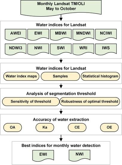
The sample points of each land use type in the two study regions were selected according to the actual distribution and the approximate area proportion. The land use types included water, wetland, paddy field, dryland, woods, grassland, construction lands and unused land. The numbers of samples of each land use type are listed in

Table 3. The sample numbers of different land use types.

Land Use Type	Number of Samples
	Chagan Lake	Songhua Lake
Water	100	135
Wetland	45	-
Paddy field	100	80
Dryland	120	100
Woods	40	160
Grassland	50	-
Construction land	90	80
Unused land	30	-

, and the positions of the reference samples are shown in Figure 1d,e. These samples were used in two respects. On the one hand, the values of the calculated water indices of the sample points were extracted, and the separability of water indices between water and the seven other background non-water land use types were evaluated. On the other hand, the seven background land use types were merged into one type named “non-water” and the samples of non-water type were used together to evaluate the water extraction accuracy based on samples. The water extraction results corresponding to the water and non-water sample points were extracted, and the overall accuracy, Kappa coefficient, commission error, and omission error were employed to quantify water extraction accuracy.

2.3. Methods

The method in this study included four steps: (1) deriving the multispectral water indices for different months; (2) obtaining the optimal segmentation thresholds of the indices for water extraction based on the adaptive segmentation algorithm; (3) extracting surface water area based on the optimal thresholds; and (4) comparing the characteristics of the water indices from their visual inter-class separability, sensitivity of segmentation thresholds, robustness of optimal thresholds and the accuracy of water extraction.

2.3.1. Calculating Multispectral Water Indices

The water index is usually a function of the TOA radiance or surface reflectance of certain bands. In previous studies, a variety of water indices have been constructed, with different equation structures, a different number of bands and different combinations of bands. In this study, we only took into consideration the water indices based on the surface reflectance of Landsat bands or those that could be calculated by the Landsat bands and calculated them first. The Pearson simple correlation analysis was applied to find the most relevant groups of indices. Considering the complementarity of the equation structures and the bands selected, ten representative indices with low correlation were selected, namely, AWEI (including AWEIsh and AWEInsh), EWI, MBWI, MNDWI, NCIWI, NDWI3, NWI, SWI, WRI, and IWS (

Table 4. Calculation equation and source references for representative water indices.

Index	Equation	Reference
AWEI	AWEInsh: 4 × (Green−SWIR1) − (0.25 × NIR + 2.75 × SWIR2)	[23]
	AWEIsh: Blue + 2.5 × Green − 1.5 × (NIR + SWIR1) − 0.25 × SWIR2
EWI	(Green − NIR − SWIR1)/(Green + NIR + SWIR1)	[17]
MBWI	2 × Green−Red−NIR − SWIR1 − SWIR2	[22]
MNDWI	(Green−SWIR1)/(Green + SWIR1)	[16]
NCIWI	(NIR − Red)/(NIR + Red) + NIR + SWIR1 + SWIR2	[45]
NDWI3	(NIR − SWIR1)/(NIR + SWIR1)	[46]
NWI	(Blue − NIR − SWIR1 − SWIR2)/(Blue + NIR + SWIR1 + SWIR2)	[18]
SWI	Blue + Green − NIR	[31]
WRI	(Green + Red)/(NIR + SWIR1)	[21]
IWS	2 × (4 × SWIR1 − Blue)/SWIR1 − 2 × SWIR1/Blue 1	[20]

¹ Note: Blue, Green, Red, NIR, SWIR1, and SWIR2 indicate the blue band, green band, red band, near-infrared band, and short-wave infrared bands one and two of Landsat surface reflectance imagery, respectively.

). Among them, NDWI and MNDWI range from −1 to 1, while water indices such as AWEI may exceed this range. To facilitate the extraction of optimal segmentation thresholds and the comparison of all indices under a unified standard, we normalized the indices and scaled them to a range from −1 to 1.

2.3.2. Obtaining Optimal Segmentation Thresholds Using the OTSU Algorithm

The OTSU algorithm is one of the most efficient and popular adaptive algorithms for deriving the optimal threshold. It divides the image into the target and the background and chooses the optimal segmentation threshold that provides the maximum inter-class variance between these two classes. The procedure is very simple and effective at producing the best segmentation result for images with double peaks in the gray histogram [47]. Sometimes, however, this algorithm cannot effectively handle the noises in the images or produce good results for images without bimodal features [32]. In this study, mean filtering with a window of 5 × 5 pixels was adopted to handle the noises, and the traditional one-dimensional OTSU algorithm was selected to obtain the optimal threshold of each index image to separate water and the non-water type. The principle of the OTSU algorithm in this study is as follows.

Assume one original water index image is an M × N image with a gray level of 0 to L − 1. The image is represented by g(x), where x is the gray level of a pixel. After the mean filtering, the image of mean value in neighborhood is obtained and represented by g(y), where y is the gray level of a pixel. Let the number of the pixels belonging to the ith gray level be denoted by n_i, and the probability of the ith gray level is expressed as follows:

$$P_i=\frac{n_i}{M\times N}, \left(i=0,1,\dots ,L-1\right),$$

(2)

where P_i denotes the probability of the ith gray level, and M × N denotes the total number of pixels of g(y). A threshold T (T ∈ [0, L − 1]) is adopted to divide the gray level image into two classes. One is a background class denoted by D_0, containing the pixels with gray levels no less than T. The other is the target class denoted by D₁ containing all the other pixels of the gray level image. The average gray values of D₀, D₁ and the entire image, which are denoted by µ₀, µ₁ and µ_T, can be expressed as follows:

$${\mu }_0={\sum }_{i=0}^T\frac{i{P}_i}{{\omega }_0}, {\mu }_1={{\displaystyle \sum }}_{i=T+1}^{L-1}\frac{i{P}_i}{{\omega }_1}, {\mu }_T={\omega }_0{\mu }_0+{\omega }_1{\mu }_1,$$

(3)

where ω₀ and ω₁ denote the cumulative probabilities of the gray levels in D₀ and D₁, respectively, and can be expressed as:

$${\omega }_0={{\displaystyle \sum }}_{i=0}^T{P}_i, {\omega }_1={{\displaystyle \sum }}_{i=T+1}^{L-1}{P}_i=1-{\omega }_0.$$

(4)

The inter-class variance between D₀ and D₁ denoted by σ² is expressed as follows:

$${\sigma }^2={\omega }_0{\left({\mu }_T-{\mu }_0\right)}^2+{\omega }_1{\left({\mu }_T-{\mu }_1\right)}^2.$$

(5)

The threshold that maximizes σ² is selected as the optimal segmentation threshold and is denoted by T_opt.

For the water index imagery with the values of water larger than the non-water type, the pixels whose values are larger than T_opt are identified as pixels of water, and the other pixels are identified as pixels of non-water type. For the index imagery with values of water smaller than those of the non-water type, the pixels whose values are smaller than T_opt are identified as pixels of water.

Before applying the OTSU algorithm, the water index images of May, July, and October 2000 were selected for validation. The results were compared with the results obtained by the two-dimensional OTSU (2D-OTSU) algorithm based on a line intercept histogram and a weighted one-dimensional OTSU (WOTSU) algorithm.

In the 2D-OTSU algorithm, both of the images g(x) and g(y) mentioned above were used to establish the criteria considering two dimensional gray levels to improve its ability to deal with noise [48]. Its principle is as follows.

Let x and y be the gray level of a certain pixel in g(x) and g(y), respectively, forming a pair of pixels. Let the sum of x and y be equal to k; the probability of the kth gray level is expressed as follows:

$$P_k=\frac{n_k}{M\times N}, \left(k=0,1,\dots ,2\left(L-1\right)\right),$$

(6)

where n_k is the number of pixel pairs meeting the equation of the line x + y = k. The intercept of the line is the segmentation threshold T dividing the gray level into D₀ and D₁. ω₀, ω₁, µ₀, and µ₁ are expressed as:

$${\omega }_0={{\displaystyle \sum }}_{k=0}^{T-1}{P}_k, {\omega }_1=1-{\omega }_0, {\mu }_0={{\displaystyle \sum }}_{k=0}^{T-1}\left(k\frac{P_k}{{\omega }_0}\right), {\mu }_1={{\displaystyle \sum }}_{k=T+1}^{2\left(L-1\right)}\left(k\frac{P_k}{{\omega }_1}\right).$$

(7)

Similar to the OTSU algorithm, the threshold that maximizes σ² is selected as the optimal segmentation threshold denoted by T_opt. After the T_opt is selected, the pixels of water are determined based on the same rule with the OTSU algorithm.

The WOTSU algorithm adopted in this study is an improved one dimensional OTSU. It takes ω₀ and ω₁ as the weight of variance of background and target, respectively. The improved σ² are expressed as follows:

$${\sigma }^2={\omega }_0{\omega }_0{\left({\mu }_T-{\mu }_0\right)}^2+{\omega }_1{\left({\mu }_T-{\mu }_1\right)}^2$$

(8)

$${\sigma }^2={\omega }_0{\left({\mu }_T-{\mu }_0\right)}^2+{\omega }_1{\omega }_1{\left({\mu }_T-{\mu }_1\right)}^2.$$

(9)

For a certain water index image, the equation of σ² is selected based on the relationship between variance of background and target. In this way, the WOTSU algorithm improves its performance in dealing with images without bimodal features [49,50].

2.3.3. Surface Water Mapping and Accuracy Analysis Method

The obtained optimal segmentation thresholds were applied to the index images to divide them into water and non-water types.

We constructed a classification confusion matrix and calculated four statistical indicators of accuracy, i.e., the overall accuracy (OA), kappa coefficient (Ka), commission error (CE), and omission error (OE), for the evaluation of water extraction accuracy based on the samples and also further usage in other analysis [51]. The specific calculations are as follows:

$$OA=\frac{TP+TN}{TA}$$

(10)

$$Ka=\frac{TP+TN-\left[\left(TP+FP\right)\left(TP+FN\right)+\left(FN+TN\right)\left(FP+TN\right)\right]}{T{A}^2-\left[\left(TP+FP\right)\left(TP+FN\right)+\left(FN+TN\right)\left(FP+TN\right)\right]}$$

(11)

$$CE=\frac{FP}{TP+FP}$$

(12)

$$OE=\frac{FN}{TP+FN},$$

(13)

where TA denotes the total number of samples, TP denotes the number of correctly identified water pixels, TN denotes the correctly rejected non-water pixels, FP denotes the number of incorrectly identified water pixels, and FN denotes the number of incorrectly identified non-water pixels.

3. Results

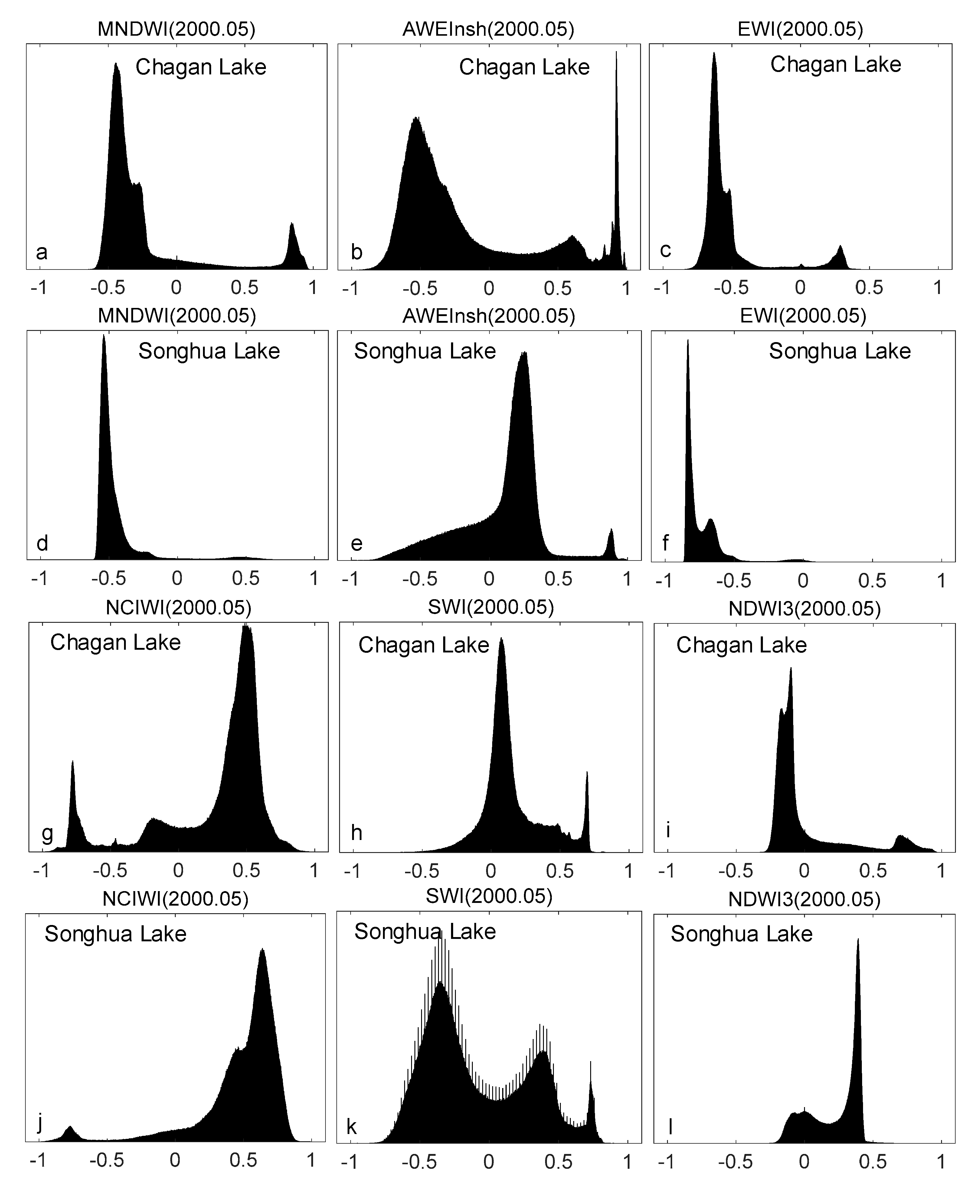
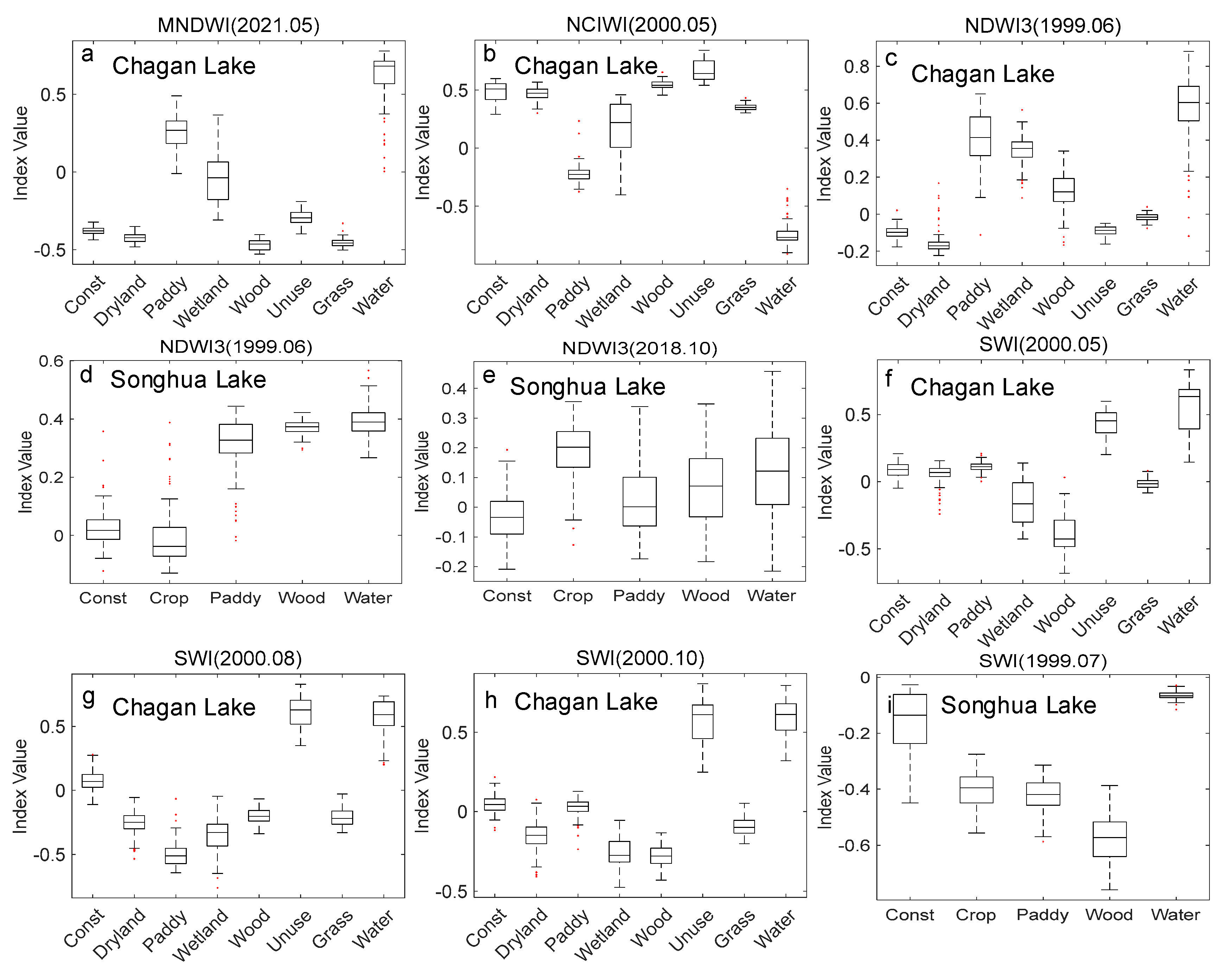
3.1. Visual Analysis of Inter-Class Separability

Ten spectral water indices (AWEI, EWI, MBWI, MNDWI, NCIWI, NDWI3, NWI, SWI, WRI, and IWS) were selected to enhance the difference between the water and non-water types. The index images of May 2000 (Chagan Lake area) and 1998 (Songhua Lake area) are shown in Figure 2 as an example. Generally, except in the NCIWI and IWS images, where the values of the water pixels are smaller than those of the other non-water types, water pixels in the other water index images have larger values than the other types. All water indices selected in this study can enhance the contrast between water and non-water types, among which the enhancement effects of SWI, NDWI3 and IWS are the weakest. The water in pixels of water-related land use types, such as paddy fields and wetlands in the study area of Chagan Lake, are also enhanced in the AWEI, MBWI, MNDWI, NDWI3, NCIWI, EWI, and NWI images, making it easy for recognition. With the first four indices above, the pixel values of paddy fields and wetlands are close to the values of water pixels. With the last three indices, the pixel values of these two types are closer to the other non-water types. In the SWI (Figure 2j), WRI (Figure 2k), and IWS (Figure 2l) images, the water information in paddy fields and wetlands is better suppressed, making it difficult to recognize from the other non-water types. For the study area of Songhua Lake, in most indices except in the NDWI3, the index values in the mountainous area are quite different from those of water bodies, or are at least close to the non-water types in plain area. However, in the NDWI3 (Figure 2t), the non-water types in the mountainous area acquire values that are quite different from the values in the plain area. NDWI3 failed to eliminate the influence of terrain factors on index value.

The index images of August 2021 (Chagan Lake area) and 2022 (Songhua Lake area) were selected as an example of the high-water period from July to September, as shown in Figure 3. In the IWS image, only a small part of Chagan Lake and the cloud can be visually recognized, thus failing to identify water (Figure 3l,x). During the high-water period in study area of Chagan Lake, the values of paddy fields and wetlands in most water index images are closer to the non-water land use types covered by vegetation. In the October images of the two years, the values of the paddy fields are also similar to the other non-water types, as shown in Figure 3.

The images acquired in August are usually contaminated by cloud. In August 2021, even though the multispectral image is mosaicked by three different images, there is still a thick cloud with dark shadows in the northeast part of the study area of Chagan Lake. In the WRI image (Figure 3k,w), the values of clouds and shadows are small and consistent with other land use types, indicating that clouds can be effectively suppressed with this index. In other water index images, a clear difference between clouds and other land use types can be observed, and clouds can also be separated from the water bodies to a certain extent. In AWEIsh (Figure 3c,o) and SWI (Figure 3j,v) images, the values of water bodies range between thick clouds and other land use types, rendering it ineffective to separate water bodies by setting only one threshold. With other water indices, the cloud areas have the largest values (Figure 3g,s), the smallest values (Figure 3h,l,t,s), or values between water bodies and other land use types (Figure 3d,f,i,p,r,u), making the water bodies effectively separated by setting one threshold.

The gray histograms of some water index images of the two study regions in May 2000 and July 2000 are shown in Figure 4 and Figure 5 as examples. By adopting certain equations, the differences of surface reflectance within the water and non-water types are suppressed and the difference between these two types is enlarged to obtain more concentrated values.

The gray histograms of the index images usually show two peaks, one of which is the histogram of water, such as the left peak of the images of NCIWI (Figure 4g,j and Figure 5g,j) and the right peak of the index images with larger values of water; the other is of a non-water type. By setting a threshold that can separate the two peaks, the water bodies and other non-water types can be separated. As the land use types in the study area of Chagan Lake are more complex, the shapes of the histogram in this area are more complex than the ones acquired by the same index at the same period of time in the study area of Songhua Lake. Even though some peaks of the water are quite low due to the small proportion of water in the whole region (Figure 4c,d,f and Figure 5d,f), most of the images show bimodal features. The distances of the two peaks of MNDWI (Figure 4a,d and Figure 5a,d), EWI (Figure 4c,f and Figure 5c,f) and NWI are long, which makes it easy to set the threshold to separate water. The shapes of the gray histograms of a certain water index acquired in different periods of time show similarities to some extent. However, for NDWI3 (Figure 4i,l and Figure 5i,l) and SWI (Figure 4h,k and Figure 5h,k), sometimes the shape of the histogram changes a lot and the peaks are close to each other, which makes it hard to apply a threshold method to find a stable and reliable threshold.

For each land use type, pixels of the water indices in different months were sampled. Part of the value distributions is shown in Figure 6. The inter-class separability between water bodies and other background land use types was analyzed. As the IWS index failed to enhance water in some situations, this section discusses all water indices except IWS. In most water index images, the value distribution of the samples resembles the distribution in Figure 6a,b. The values of water are either the largest (in the AWEIsh, AWEInsh, EWI, MBWI, MNDWI, NWI, and WRI images of the test months) or the smallest (in the NCIWI images of all the test months), which is far from the value distribution of other types. Most indices can distinguish between water bodies and non-water types during the high- and low-water periods. However, during the water-stable period from April to June, the maximum or minimum index values of paddy fields and wetlands may overlap with those of water bodies. In addition, in the NDWI3 image, the values of water show overlapping with the other non-water types during the high-water period and low-water period (Figure 6c–e). With the NDWI3 of October 2018 in the study area of Songhua Lake, the water pixels were confused with all the other land cover types. That is because the water appeared in different colors in different parts across the area at that time. This may indicate that NDWI3 may fail to cope with polluted water with different water colors. With the SWI of all six test months, the maximum or minimum index values of water overlap with the unused land in the study area of Chagan Lake (Figure 6d–i) and overlap with the construction land in the study area of Songhua Lake. With SWI, the water pixels may be confused with pixels of little vegetation cover. Based on the comprehensive comparison of all the samples, NDWI3 and SWI cannot effectively separate water from the background types and are unsuitable for water extraction in these regions.

3.2. Analysis of Segmentation Threshold

3.2.1. Sensitivity of Segmentation Threshold

Based on the characteristics of the water indices, researchers often manually set the segmentation threshold to 0 for water body extraction. In this section, the water index images of May (water-stable period), July (high-water period), and October (low-water period of Chagan Lake and the second water-stable period of Songhua Lake) were selected. With an empirical threshold of 0 as the center, 37 values ranging from −0.9 to 0.9 with a step of 0.05 were set as segmentation thresholds. The OA and Ka of the water extraction results under each threshold were calculated to analyze the sensitivity of the segmentation threshold for each water index. The results of the two study areas show similar trends and the results of Chagan Lake are shown as examples in Figure 7. For all indices, the optimal threshold to obtain the largest water extraction accuracy varies with time and is within certain ranges during different periods. To obtain the most accurate water extraction results, certain methods are required to obtain the optimal segmentation threshold first. Other than SWI, most indices are more sensitive to the threshold during the water-stable period (Figure 7a,d,g,j), and the value ranges for the optimal thresholds are narrower. During the other two periods, indices such as MNDWI (Figure 7b,c), AWEI (Figure 7e,f), EWI (Figure 7h,i), NWI, and NCIWI can maintain high accuracy when the thresholds are set within a certain range overlapping with the ranges of the water-stable period. After achieving their optimal thresholds of the water-stable period, the thresholds can be applied to images of the other periods. Nevertheless, other indices, such as SWI (Figure 7j–l) and NDWI3, have significantly varying value ranges. When extracting surface water for different periods, experiments for every period are required to determine the optimal segmentation threshold first.

3.2.2. Robustness of the Optimal Threshold

As the gray histogram of most index images showed bimodal features (Figure 4 and Figure 5), in this study, the traditional one-dimensional OTSU algorithm was used to automatically extract the optimal segmentation threshold of each water index image. Before applying the algorithm, the water index images of May, July, and October 2000 were selected for validation. The results were compared with the results acquired using the two-dimensional OTSU algorithm (2D-OTSU) based on a line intercept histogram and the weighted one-dimensional OTSU algorithm (WOTSU) based on OA and Ka, respectively [52]. As shown in Figure 8, in the study area of Chagan Lake, when the threshold values of MNDWI and NCIWI extracted by the OTSU algorithm were used for water extraction, the OA of the results was nearly the highest, with the Ka exceeding 0.4, indicating good classification results. For the other indices, the results achieved by the 2D-OTSU algorithm have the highest OA during the water-stable period. During the high- and low-water periods, even though the OA achieved by the one-dimensional OTSU algorithm is not always the largest for indices such as AWEIsh and NCIWI in July, as well as NDWI3 and NWI in October, it can still reach 0.90. Therefore, it is reasonable to adopt the one-dimensional OTSU algorithm to extract the optimal thresholds and achieve reliable results in most situations. To ensure that the best threshold is always selected for water extraction, the 2D-OTSU algorithm was applied to all index images except MNDWI and NCIWI during the water-stable period. As shown in Figure 9, the situations in the study area of Songhua Lake are different. For most water indices, the one-dimensional OTSU algorithm achieved a better performance during the two water-stable periods. However, for the indices—except NCIWI, NDWI3, SWI and WRI—the results achieved by the 2D-OTSU algorithm have the highest OA during the high-water period. To ensure that the best threshold is always selected for water extraction, the 2D-OTSU algorithm was applied to all index images except the four indices mentioned above during the high-water period. The 2D-OTSU algorithm depends on the sum of two images with values ranging from −1 to 1, respectively, and the optimal thresholds acquired by this algorithm are converted to the range from −1 to 1, which is consistent with the OTSU algorithm. After checking the results of water extraction based on the optimal segmentation thresholds, the wrong optimal thresholds of a few water indices were manually modified and used for water extraction.

The plots of optimal segmentation thresholds for water indices from May to October are shown in Figure 10. It can be observed that the curves of MNDWI and NWI are flatter than those of the others, with values ranging from 0.023 to 0.229, and from −0.539 to −0.223 in the Chagan Lake area and with values ranging from −0.085 to 0.147 and from −0.652 to −0.352 in the Songhua Lake area (Figure 10a,b). The value ranges for each index are consistent with the ranges shown in Figure 7. For Landsat images with different sensors in different periods, the difference in optimal segmentation thresholds of the two indices above is from about 0.20 to 0.31. In addition, the threshold values are relatively centralized (Figure 10c,d). After obtaining the optimal threshold of one month, it can be extended to images in other periods. When it is necessary to use the empirical threshold to extract water bodies, the indices with the stable optimal threshold under different scenarios are good choices for carrying out the work. For the other indices, especially AWEInsh, SWI, and WRI, the curves fluctuate greatly with time and may change a lot in different situations. For these indices, optimal threshold experiments for different periods are required to obtain higher water extraction accuracy.

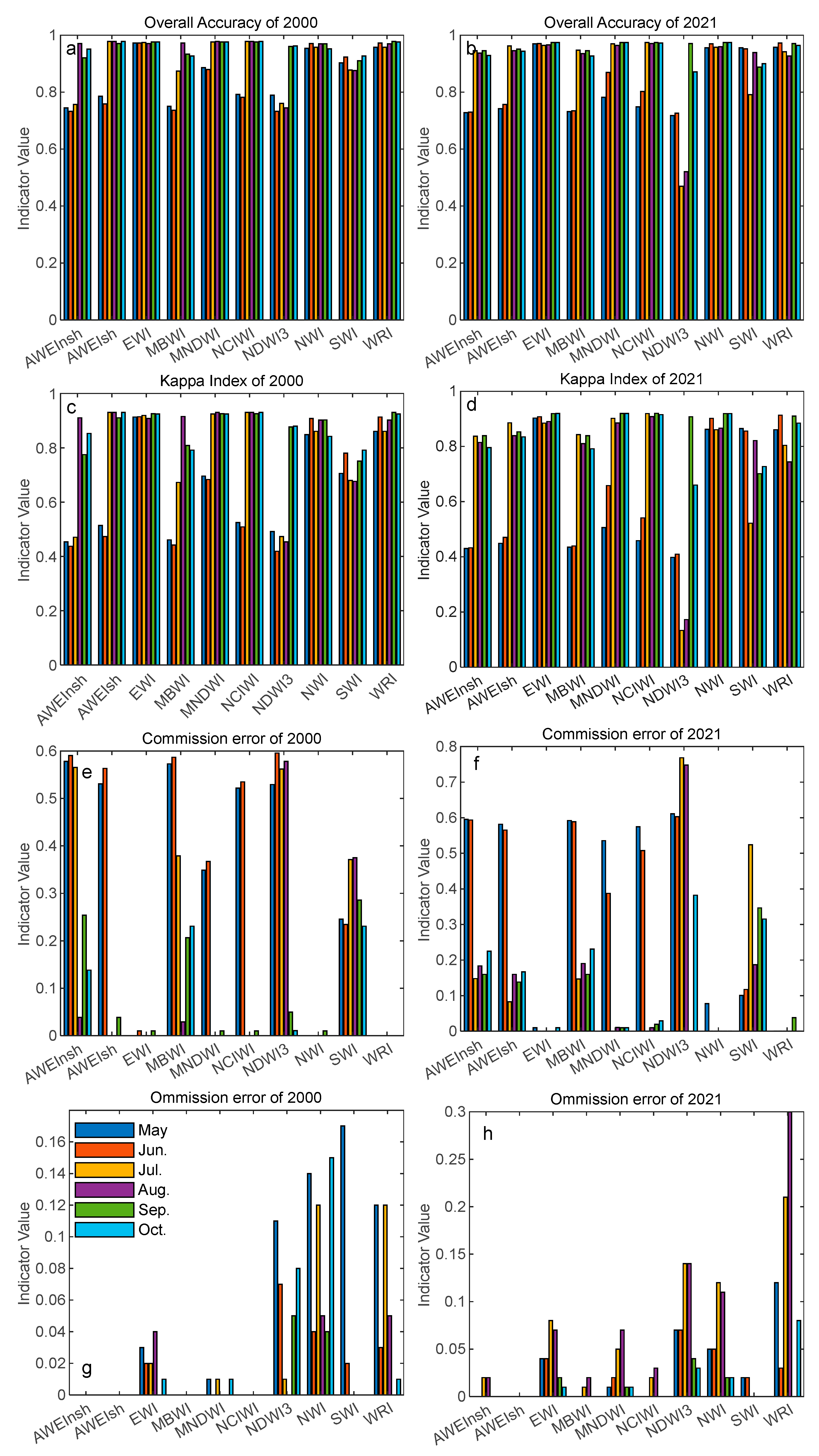
3.3. The Accuracy of Water Extraction

The optimal thresholds of each index were used to identify surface water bodies, and OA, Ka, CE, and OE were used to evaluate the extraction accuracy. The plots of these statistical indicators are shown in Figure 11 and Figure 12, and some of the water maps are shown in Figure 13 and Figure 14. In Figure 13 and Figure 14, some of the sections are selected and marked to help us focus on certain regions in the study area and explain the performance of the water extraction.

In the study period in 2019, all the indices performed well in all months in terms of OA, except for NDWI3 in the study area of Songhua Lake (Figure 12b). When taking all the cases into account, EWI, NWI, and WRI perform the best in all months in terms of OA, followed by SWI with an OA of over 0.80. The NDWI3 performs the worst in most months, especially during the high-water period. AWEI, MBWI, and NCIWI usually perform badly during the water-stable period (Figure 11a,b and Figure 12a).

CE shows the percentage of incorrectly identified non-water samples to all samples ascertained as water. In the study area of Chagan Lake, all indices except EWI, NWI and WRI achieve significant CEs during the water-stable period. Additionally, NDWI3 and SWI have CEs of 56.2% to 76.4% and 18.7% to 52.4% in July and August during the high-water period. In terms of the entire images, the AWEInsh, MBWI, MNDWI, NCIWI, and NDWI3 images during the water-stable period show pixels of paddy fields (within sections C and D in Figure 13) and wetlands (within sections E and F in Figure 13) incorrectly classified as water (Figure 13c–f). In the SWI images, pixels of unused lands (within sections A and B in Figure 13) are also classified as water (Figure 13h,z). Among all indices, EWI, NCIWI, MNDWI, NWI, and WRI can suppress the information of clouds (within section I in Figure 13) to a certain extent (Figure 13k–n,p,r, section A). In the study area of Songhua Lake, even EWI and WRI in the study period of 1999 achieved CEs to some extent during the first water-stable period. NWI have CEs of 0 to 7%. EWI and WRI have CEs of 0 to 28.2% and of 0% to 27%. Even though their CEs are higher than those of NWI, they are still at a relatively low level. In terms of the entire images, the water maps based on these indices usually show pixels of construction land (within section M in Figure 14) and the aspects of the mountains (within section N in Figure 14) incorrectly classified as water.

OE shows the percentage of incorrectly identified water samples to all actual water samples. In the study area of Chagan Lake, the OE during the high-water period in 2021 is above that of the other periods. The CEs of July and August WRI during the high-water period in 2021 range from 20% to 30%, but the CEs of all other cases are below 20% (Figure 11e,f). Only a few water samples are classified as non-water types. EWI, NDWI3, NWI, SWI, and WRI have larger OEs than the other indices. Even though most of the water bodies can be effectively identified, water pixels in the narrow rivers (within sections G and H in Figure 13) are still missed (Figure 13b,d,f–i), as are the pixels of small water bodies. Comprehensively comparing all the indices, NWI and EWI still perform the best for the study area. In the study area of Songhua Lake, this usually happened in May and June when the water body is narrow.

4. Discussion

The results show that the water pixels of water-related land use types, such as paddy fields and wetlands, are also enhanced in the AWEI, MBWI, MNDWI, NDWI3, NCIWI, EWI, and NWI images of May and June during the water-stable period. The pixels of paddy fields and wetlands show similar features to the pixels of water during this period. In the study area of Chagan Lake, the marsh is mainly at the northwest edge of Chagan Lake and Xindian Lake, as well as the edge of Xinmiao Lake (Figure 1). The main vegetation types of the marsh are reed, Phragmites australis, and Typha angustifolia, with surface water coverage [43,44]. The paddy fields are mainly distributed in the Qianguo irrigated area (in the east of the region) and the Da’an irrigated area (in the northwest corner of the region), respectively (Figure 1b). Due to the irrigation, the paddy fields also contain a certain amount of surface water in the early growing season and appear dark green in the Landsat multispectral imagery acquired in May and early June. During this period, the vegetation is in the early growing season, and the fractions of vegetation coverage in each pixel of these two types are low, resulting in incorrect identification.

This study used Landsat imagery as the data source and calculated 10 water indices. The optimal segmentation threshold characteristics and the water extraction performance of each index during the vegetation growing season were investigated. Other than IWS and NDWI3, all other indices performed well in separating water from non-water types by setting one single threshold for the entire index image of the study area. Previous studies have found that the OTSU algorithm is unsuitable for AWEI [53]. In this study, it depends; in the study area of Chagan Lake, even though the background land cover types are complex, the threshold obtained by OTSU could help separate water and non-water type-. The Ka of water extraction by AWEI is above 0.4, and the OA of water extraction based on the reference samples is above 0.75. The optimal threshold of AWEI extracted in this study is also reliable. Nevertheless, if other algorithms were adopted to determine the threshold of AWEI, the accuracy may be higher. However, in the study area of Songhua Lake, the optimal thresholds in May obtained by all the three algorithms failed to identify water. Among the indices, SWI was developed based on Sentinel-2 data, which has achieved a better performance than NDWI in previous studies. In this study, SWI was calculated using the corresponding bands of Landsat imagery, which shows a certain water extraction ability. However, water bodies cannot be separated from saline-alkali areas and construction areas in the study area. The calculation of SWI based on Landsat images may affect its performance, making it unable to accurately extract water bodies in saline areas or near construction lands.

The results show that, when taking all the results of the two study areas into consideration, MNDWI, NWI, and EWI achieved relatively stable optimal thresholds during the vegetation growing seasons and produced the best water extraction performances. They are all ratio based indices which increase the values of water by taking the bands with low reflectance of water as the denominator and the bands with high reflectance as the numerator. As mentioned before, the MNDWI replaced the NIR band in NDWI with the SWIR1 band of Landsat TM to enhance the water signal. No matter whether the water is clear or not, its reflectance of the NIR band and SWIR1 band is very low. The scholars replaced the SWIR1 band in MNDWI with the sum of NIR and SWIR1 and built EWI. The water pixels could always reach larger positive values in EWI, while the backgrounds were suppressed. This characteristic makes EWI robust when applied to the polluted water bodies such as Chagan Lake and Songhua Lake. Moreover, after replacing the sum of NIR and SWIR1 with the sum of three bands, NIR, SWIR1 and SWIR2, and replacing the Green band in EWI with the Blue band, the index value of water pixels was further enlarged, making the water easy to recognize and separated from the background.

In the study area of Chagan Lake, as shown in Figure 8, the optimal thresholds adopted in this study can lead to the best water extraction performance for EWI and MNDWI in all test months, but the 2D-OTSU algorithm could achieve a better performance for NWI. The optimal segmentation thresholds of NWI obtained by the two algorithms are shown in Figure 15. The thresholds produced by 2D-OTSU are smaller than those of OTSU. The difference between the optimal segmentation thresholds of May 2021 obtained by the two algorithms is −0.0448 and below 0.01 for other months.

The resultant maps of NWI based on the optimal thresholds calculated by the two algorithms are shown in Figure 16. In most cases, the difference between the optimal segmentation thresholds obtained by the two methods has little impact on the water extraction accuracy. However, in the case of May 2021, a large number of paddy field pixels were misclassified as water types using the optimal segmentation thresholds obtained by the 2D-OTSU algorithm. Therefore, it is reasonable to adopt the method in this research to obtain the optimal segmentation threshold, and conclude that the NWI optimal threshold is stable at different times is reliable.

5. Conclusions

Using Landsat TM and OLI multispectral data as data sources, 10 water indices were calculated. The OTSU algorithm was adopted to automatically extract the optimal segmentation thresholds for regional water body extraction. Each water index was analyzed in terms of inter-class separability, threshold sensitivity, optimal threshold robustness, and water extraction accuracy. The following conclusions were obtained:

Each water index can enhance water information and suppress background information. Specifically, NWI, EWI, WRI, MNDWI, and NCIWI can achieve the best enhancement effect, while SWI and IWS have the weakest enhancement effect.

The water extraction accuracy of MNDWI, EWI, and NWI is less sensitive to the threshold than the other indices. The optimal segmentation thresholds in different periods fluctuate less. Once the optimal values of the water-stable period are achieved, the values can be applied to other periods of the year.

EWI and NWI have the highest water extraction accuracy in the two study areas. Based on the optimal threshold, they achieved an OA of 0.952 to 0.981 and 0.964 to 0.981, respectively. The CE is 0 to 28.2% and 0 to 7.7%, the OE is 0 to 15% and 0 to 8%, and the Ka is over 0.8, indicating good extraction results. With the other water indices, water pixels are often confused with non-water land use types in different periods of the year, and their applicability in this region is relatively poor. During water extraction based on SWI, water bodies are often confused with unused land, while in water extraction based on other indices, water bodies are confused with water-related types, such as paddy fields and wetlands, during the water-stable period. To sum up, EWI and NWI have the best water extraction effect in the study area. Even though this study only focused on two specific regions in Jilin Province, these indices have the potential for accurately monitoring the surface water over other regions.

References

1. Palmer, S.C.J.; Kutser, T.; Hunter, P.D. Remote sensing of inland waters: Challenges, progress and future directions. Remote Sens. Environ. 2015, 157, 1–8. [Google Scholar] [CrossRef] [Green Version]
2. Li, J.; Ma, R.; Cao, Z.; Xue, K.; Xiong, J.; Hu, M.; Feng, X. Satellite Detection of Surface Water Extent: A Review of Methodology. Water 2022, 14, 1148. [Google Scholar] [CrossRef]
3. Khalid, H.W.; Khalil, R.M.Z.; Qureshi, M.A. Evaluating spectral indices for water bodies extraction in western Tibetan Plateau. Egypt. J. Remote Sens. Space Sci. 2021, 24, 619–634. [Google Scholar] [CrossRef]
4. Quang, D.N.; Linh, N.K.; Tam, H.S.; Viet, N.T. Remote sensing applications for reservoir water level monitoring, sustainable water surface management, and environmental risks in Quang Nam province, Vietnam. J. Water Clim. Chang. 2021, 12, 3045–3063. [Google Scholar] [CrossRef]
5. Li, A.; Fan, M.; Qin, G.; Xu, Y.; Wang, H. Comparative Analysis of Machine Learning Algorithms in Automatic Identification and Extraction of Water Boundaries. Appl. Sci. 2021, 11, 10062. [Google Scholar] [CrossRef]
6. Loudière, D.; Gourbesville, P. Rapport mondial des Nations Unies sur la mise en valeur des ressources en eau 2020. La Houille Blanche 2020, 106, 76–81. [Google Scholar] [CrossRef]
7. Wang, G.; Wu, M.; Wei, X.; Song, H. Water Identification from High-Resolution Remote Sensing Images Based on Multidimensional Densely Connected Convolutional Neural Networks. Remote Sens. 2020, 12, 795. [Google Scholar] [CrossRef] [Green Version]
8. Yang, X.; Qin, Q.; Yésou, H.; Ledauphin, T.; Koehl, M.; Grussenmeyer, P.; Zhu, Z. Monthly estimation of the surface water extent in France at a 10-m resolution using Sentinel-2 data. Remote Sens. Environ. 2020, 244, 111803. [Google Scholar] [CrossRef]
9. Herndon, K.; Muench, R.; Cherrington, E.; Griffin, R. An Assessment of Surface Water Detection Methods for Water Resource Management in the Nigerien Sahel. Sensors 2020, 20, 431. [Google Scholar] [CrossRef] [Green Version]
10. Li, M.; Hong, L.; Guo, J.; Zhu, A. Automated Extraction of Lake Water Bodies in Complex Geographical Environments by Fusing Sentinel-1/2 Data. Water 2021, 14, 30. [Google Scholar] [CrossRef]
11. Kseňak, Ľ.; Pukanská, K.; Bartoš, K.; Blišťan, P. Assessment of the Usability of SAR and Optical Satellite Data for Monitoring Spatio-Temporal Changes in Surface Water: Bodrog River Case Study. Water 2022, 14, 299. [Google Scholar] [CrossRef]
12. Guo, Z.; Wu, L.; Huang, Y.; Guo, Z.; Zhao, J.; Li, N. Water-Body Segmentation for SAR Images: Past, Current, and Future. Remote Sens. 2022, 14, 1752. [Google Scholar] [CrossRef]
13. Xiong, L.; Deng, R.; Li, J.; Liu, X.; Qin, Y.; Liang, Y.; Liu, Y. Subpixel Surface Water Extraction (SSWE) Using Landsat 8 OLI Data. Water 2018, 10, 653. [Google Scholar] [CrossRef] [Green Version]
14. Li, L.; Su, H.; Du, Q.; Wu, T. A novel surface water index using local background information for long term and large-scale Landsat images. ISPRS J. Photogramm. Remote Sens. 2021, 172, 59–78. [Google Scholar] [CrossRef]
15. McFeeters, S.K. The use of the Normalized Difference Water Index (NDWI) in the delineation of open water features. Int. J. Remote Sens. 1996, 17, 1425–1432. [Google Scholar] [CrossRef]
16. Xu, H. Modification of normalised difference water index (NDWI) to enhance open water features in remotely sensed imagery. Int. J. Remote Sens. 2006, 27, 3025–3033. [Google Scholar] [CrossRef]
17. Yan, P.; Zhang, Y. A Study on Information Extraction of Water System in Semi-arid Regions with the Enhanced Water Index (EWI) and GIS Based Noise Remove Techniques. Remote Sens. Inf. 2007, 6, 62–67. [Google Scholar]
18. Ding, F. A New Method for Fast Information Extraction of Water Bodies Using Remotely Sensed Data. Remote Sens. Technol. Appl. 2009, 24, 167–171. [Google Scholar]
19. Fisher, A.; Flood, N.; Danaher, T. Comparing Landsat water index methods for automated water classification in eastern Australia. Remote Sens. Environ. 2016, 175, 167–182. [Google Scholar] [CrossRef]
20. Hassani, M.; Chabou, M.C.; Hamoudi, M.; Guettouche, M.S. Index of extraction of water surfaces from Landsat 7 ETM+ images. Arab. J. Geosci. 2015, 8, 3381–3389. [Google Scholar] [CrossRef]
21. Shen, L.; Li, C. Water body extraction from Landsat ETM+ imagery using adaboost algorithm. In Proceedings of the 2010 18th International Conference on Geoinformatics, Beijing, China, 18–20 June 2010; pp. 1–4. [Google Scholar]
22. Wang, X.; Xie, S.; Zhang, X.; Chen, C.; Guo, H.; Du, J.; Duan, Z. A robust Multi-Band Water Index (MBWI) for automated extraction of surface water from Landsat 8 OLI imagery. Int. J. Appl. Earth Obs. Geoinf. 2018, 68, 73–91. [Google Scholar] [CrossRef]
23. Feyisa, G.L.; Meilby, H.; Fensholt, R.; Proud, S.R. Automated Water Extraction Index: A new technique for surface water mapping using Landsat imagery. Remote Sens. Environ. 2014, 140, 23–35. [Google Scholar] [CrossRef]
24. Xie, C.; Huang, X.; Zeng, W.; Fang, X. A novel water index for urban high-resolution eight-band WorldView-2 imagery. Int. J. Digit. Earth 2016, 9, 925–941. [Google Scholar] [CrossRef]
25. Wen, Z.; Zhang, C.; Shao, G.; Wu, S.; Atkinson, P.M. Ensembles of multiple spectral water indices for improving surface water classification. Int. J. Appl. Earth Obs. Geoinf. 2021, 96, 102278. [Google Scholar] [CrossRef]
26. Sanchez, G.C.; Dalmau, O.; Alarcon, T.E.; Sierra, B.; Hernandez, C. Selection and Fusion of Spectral Indices to Improve Water Body Discrimination. IEEE Access 2018, 6, 72952–72961. [Google Scholar] [CrossRef]
27. Ferriby, H.; Nejadhashemi, A.P.; Hernandez-Suarez, J.S.; Moore, N.; Kpodo, J.; Kropp, I.; Eeswaran, R.; Belton, B.; Haque, M.M. Harnessing Machine Learning Techniques for Mapping Aquaculture Waterbodies in Bangladesh. Remote Sens. 2021, 13, 4890. [Google Scholar] [CrossRef]
28. Yu, Z.; Di, L.; Rahman, M.S.; Tang, J. Fishpond Mapping by Spectral and Spatial-Based Filtering on Google Earth Engine: A Case Study in Singra Upazila of Bangladesh. Remote Sens. 2020, 12, 2692. [Google Scholar] [CrossRef]
29. Rokni, K.; Ahmad, A.; Selamat, A.; Hazini, S. Water Feature Extraction and Change Detection Using Multitemporal Landsat Imagery. Remote Sens. 2014, 6, 4173–4189. [Google Scholar] [CrossRef] [Green Version]
30. Mondejar, J.P.; Tongco, A.F. Near infrared band of Landsat 8 as water index: A case study around Cordova and Lapu-Lapu City, Cebu, Philippines. Sustain. Environ. Res. 2019, 29, 16. [Google Scholar] [CrossRef] [Green Version]
31. Jiang, W.; Ni, Y.; Pang, Z.; Li, X.; Ju, H.; He, G.; Lv, J.; Yang, K.; Fu, J.; Qin, X. An Effective Water Body Extraction Method with New Water Index for Sentinel-2 Imagery. Water 2021, 13, 1647. [Google Scholar] [CrossRef]
32. Zhou, C.; Tian, L.; Zhao, H.; Zhao, K. A method of Two-Dimensional Otsu image threshold segmentation based on improved Firefly Algorithm. In Proceedings of the 2015 IEEE International Conference on Cyber Technology in Automation, Control, and Intelligent Systems (CYBER), Shenyang, China, 8–12 June 2015; pp. 1420–1424. [Google Scholar]
33. Yin, D.; Cao, X.; Chen, X.; Shao, Y.; Chen, J. Comparison of automatic thresholding methods for snow-cover mapping using Landsat TM imagery. Int. J. Remote Sens. 2013, 34, 6529–6538. [Google Scholar] [CrossRef]
34. Sheng, Y.; Song, C.; Wang, J.; Lyons, E.A.; Knox, B.R.; Cox, J.S.; Gao, F. Representative lake water extent mapping at continental scales using multi-temporal Landsat-8 imagery. Remote Sens. Environ. 2016, 185, 129–141. [Google Scholar] [CrossRef] [Green Version]
35. Weekley, D.; Li, X. Tracking Multidecadal Lake Water Dynamics with Landsat Imagery and Topography/Bathymetry. Water Resour. Res. 2019, 55, 8350–8367. [Google Scholar] [CrossRef]
36. Wang, P.; Li, Z.; Xu, C.; Wang, P. Region-wide glacier area and mass budgets for the Shaksgam River Basin, Karakoram Mountains, during 2000–2016. J. Arid. Land 2021, 13, 175–188. [Google Scholar] [CrossRef]
37. Chen, Y.; Fan, R.; Yang, X.; Wang, J.; Latif, A. Extraction of Urban Water Bodies from High-Resolution Remote-Sensing Imagery Using Deep Learning. Water 2018, 10, 585. [Google Scholar] [CrossRef] [Green Version]
38. Zhang, Y.J.; Liu, X.Y.; Zhang, Y.; Ling, X.; Huang, X. Automatic and Unsupervised Water Body Extraction Based on Spectral-Spatial Features Using GF-1 Satellite Imagery. Ieee Geosci. Remote Sens. Lett. 2019, 16, 927–931. [Google Scholar] [CrossRef]
39. Pekel, J.-F.; Cottam, A.; Gorelick, N.; Belward, A.S. High-resolution mapping of global surface water and its long-term changes. Nature 2016, 540, 418–422. [Google Scholar] [CrossRef] [PubMed]
40. Campos, J.C.; Sillero, N.; Brito, J.C. Normalized difference water indexes have dissimilar performances in detecting seasonal and permanent water in the Sahara–Sahel transition zone. J. Hydrol. 2012, 464–465, 438–446. [Google Scholar] [CrossRef]
41. Liu, X.; Chen, L.; Zhang, G.; Zhang, J.; Wu, Y.; Ju, H. Spatiotemporal dynamics of succession and growth limitation of phytoplankton for nutrients and light in a large shallow lake. Water Res. 2021, 194, 116910. [Google Scholar] [CrossRef]
42. Zhu, X.; Yuan, Y.; Wei, X.; Wang, L.; Wang, C. Dissimilatory iron reduction and potential methane production in Chagan Lake wetland soils with carbon addition. Wetl. Ecol. Manag. 2021, 29, 369–379. [Google Scholar] [CrossRef]
43. Yang, Y.N.; Sheng, Q.; Zhang, L.; Kang, H.Q.; Liu, Y. Desalination of saline farmland drainage water through wetland plants. Agric. Water Manag. 2015, 156, 19–29. [Google Scholar] [CrossRef]
44. You, Q. Determining paddy field spatiotemporal distribution and temperature influence using remote sensing in Songnen Plain, Northeastern China. Arab. J. Geosci. 2020, 13, 1075. [Google Scholar] [CrossRef]
45. Zou, C.; Yang, X.Z.; Dong, Z.Y.; Wang, D. A Fast Water Information Extraction Method Based on GF-2 Remote Sensing Image. J. Graph. 2019, 40, 99. [Google Scholar]
46. Ouma, Y.O.; Tateishi, R. A water index for rapid mapping of shoreline changes of five East African Rift Valley lakes: An empirical analysis using Landsat TM and ETM+ data. Int. J. Remote Sens. 2006, 27, 3153–3181. [Google Scholar] [CrossRef]
47. Otsu, N. A Threshold Selection Method from Gray-Level Histograms. IEEE Trans. Syst. Man Cybern. 1979, 9, 62–66. [Google Scholar] [CrossRef] [Green Version]
48. Xiao, L.; Ouyang, H.; Fan, C. An improved Otsu method for threshold segmentation based on set mapping and trapezoid region intercept histogram. Optik 2019, 196, 163106. [Google Scholar] [CrossRef]
49. Huang, Y.; Xiong, L.; Liu, Y.; Deng, P.; Dan, B. Image segmentation of argon blowing based on improved Otsu algorithm. In Proceedings of the 2021 4th International Conference on Intelligent Autonomous Systems (ICoIAS), Wuhan, China, 14–16 May 2021; pp. 49–54. [Google Scholar]
50. Yuan, X.-C.; Wu, L.-S.; Peng, Q. An improved Otsu method using the weighted object variance for defect detection. Appl. Surf. Sci. 2015, 349, 472–484. [Google Scholar] [CrossRef] [Green Version]
51. Yan, D.; Huang, C.; Ma, N.; Zhang, Y. Improved Landsat-Based Water and Snow Indices for Extracting Lake and Snow Cover/Glacier in the Tibetan Plateau. Water 2020, 12, 1339. [Google Scholar] [CrossRef]
52. He, Z.; Sun, L.; Huang, W.; Chen, L. Thresholding segmentation algorithm based on Otsu criterion and line intercept histogram. Opt. Precis. Eng. 2012, 20, 2315–2323. [Google Scholar] [CrossRef]
53. Asfaw, W.; Haile, A.T.; Rientjes, T. Combining multisource satellite data to estimate storage variation of a lake in the Rift Valley Basin, Ethiopia. Int. J. Appl. Earth Obs. Geoinf. 2020, 89, 102095. [Google Scholar] [CrossRef]
Figure 1. Location (a) surrounding river network and main irrigated areas (b,c) and land use types and sample position (d,e) of the two study areas.
Remotesensing 15 01678 g001
Figure 2. The multispectral image and grayscale images of water indices of May 2000 and 2018.
Remotesensing 15 01678 g002
Figure 3. The multispectral image and the grayscale images of water indices of August 2021.
Remotesensing 15 01678 g003
Figure 4. Gray histogram of MNDWI (a,d), AWEInsh (b,e), EWI (c,f), NCIWI (g,j), SWI (h,k) and NDWI3 (i,l) images in May 2000 of the two study regions.
Remotesensing 15 01678 g004
Figure 5. Gray histogram of MNDWI (a,d), AWEInsh (b,e), EWI (c,f), NCIWI (g,j), SWI (h,k) and NDWI3 (i,l) images in in July 2000 of the two study regions.
Remotesensing 15 01678 g005
Figure 6. The value distributions of MNDWI (a), NCIWI (b), NDWI3 (ce) and SWI (fi) in different months of each land use type. “Const”, “Dryland”, “Paddy”, “Wetland”, “Wood”, “Unuse”, “Grass”, and “Water” in the boxplot figure represent construction land, dryland, paddy field, wetland, woods, unused land, grassland, and water body, respectively.
Remotesensing 15 01678 g006
Figure 7. OA and the Ka of water classification of MNDWI (ac), AWEIsh (df), EWI (gi) and SWI (jl) of different water periods based on different segmentation thresholds.
Remotesensing 15 01678 g007
Figure 8. Evaluation charts of OA (a,c,e) and Ka (b,d,f) of water extraction experiments for water indices of different water periods based on the optimal segmentation thresholds obtained by the three adaptive algorithms in the study area of Chagan Lake.
Remotesensing 15 01678 g008
Figure 9. Evaluation charts of OA (a,c,e) and Ka (b,d,f) of water extraction experiments for water indices of different water periods based on the optimal segmentation thresholds obtained by the three adaptive algorithms in the study area of Songhua Lake.
Remotesensing 15 01678 g009
Figure 10. Dynamics of the optimal segmentation thresholds for different indices in different months of the year in the study area of Chagan Lake (a) and Songhua Lake (b), and the value distribution of these two regions (c,d). The red crosses “+” in the value distribution charts (c,d) represent the outliers of the samples.
Remotesensing 15 01678 g010
Figure 11. Evaluation plots of the OA (a,b), Ka (c,d), CE (e,f) and OE (g,h) for water extraction in the study area of Chagan Lake based on the water indices with their optimal segmentation thresholds from May to October in 2000 and 2021, respectively.
Remotesensing 15 01678 g011
Figure 12. Evaluation plots of the OA (a,b), Ka (c,d), CE (e,f) and OE (g,h) for water extraction in the study area of Songhua Lake based on the water indices with their optimal segmentation thresholds from May to October in 2000 and 2021, respectively.
Remotesensing 15 01678 g012
Figure 13. RGB (band 752 in Table 1) images and waterextraction maps of the study area of Chagan Lake in different water periods based on AWEInsh (a,j,s), EWI (b,k,t), MBWI (c,l,u), MNDWI (d,m,v), NCIWI (e,n,w), NDWI3 (f,o,x), NWI (g,p,y), SWI (h,q,z) and WRI (i,r,A) with their optimal segmentation thresholds. The orange boxes and the red uppercase letters on the maps within the boxes (A–J) are used to mark the typical regions where CE or OE occurs.
Remotesensing 15 01678 g013
Figure 14. RGB (band 752 in Table 1) image and water extraction maps of the study area of Songhua Lake based on the AWEInsh (a), AWEIsh (b), EWI (c), MBWI (d), MNDWI (e), NCIWI (f), NDWI3 (g), NWI (h), SWI (i) and WRI (j) of May 2000 and on the MBWI (k) of October 2000 with their optimal segmentation thresholds. The orange boxes and the red uppercase letters on the maps within the box (M and N) are used to mark the typical regions where CE or OE occurs.
Remotesensing 15 01678 g014
Figure 15. Optimal thresholds of NWI calculated by two adaptive algorithms of the study area of Chagan Lake in each month of 2000 (a) and 2021 (b).
Remotesensing 15 01678 g015
Figure 16. Water extraction maps of the study area of Chagan Lake from May to October 2000 (af) and 2021 (gl) based on NWI with optimal thresholds adopted by the two algorithms.
Remotesensing 15 01678 g016