Abstract
The Environmental Trace Gases Monitoring Instrument 2 (EMI-2), a second-generation Chinese hyperspectral satellite-based spectrometer, was launched on 7 September 2021. The total ozone column (TOC) product, which is one of the most important elements of the EMI-2 mission, is required for monitoring the Antarctic ozone hole and regional tropospheric ozone pollution. The first EMI-2 TOC results using the differential optical absorption spectroscopy (DOAS) method are presented in this study. Significant improvements, such as the fitting interval, reference spectrum, and iterative air mass factor (AMF) calculation scheme, were implemented in the EMI-2 TOC retrieval in comparison with the EMI DOAS TOC algorithm, thus generating more accurate reads. The monthly average EMI-2 DOAS TOCs in November 2021 were compared with the TROPOspheric Monitoring Instrument (TROPOMI) TOCs, and the results showed a good correlation (R = 0.99). The EMI-2 TOCs showed similar global spatial distributions to those of TROPOMI, with an overall mean relative bias and mean standard deviation of 0.16% and 2.38%, respectively. However, large differences (up to 7%) appeared in some polar areas near the coastline, which were mainly caused by different surface albedo algorithms. Furthermore, ground-based measurements from 20 stations across different latitudes derived from the World Ozone and Ultraviolet Radiation Data Center dataset were used to assess the accuracy of the EMI-2 DOAS TOCs, and they had a mean relative bias and mean standard deviation of 0.70% and 3.65%, respectively. These results indicate that the EMI-2 DOAS TOC algorithm can yield reliable global TOCs and monitor daily Antarctic TOCs for assessing the healing of ozone holes.
1. Introduction
Stratospheric ozone, which is mainly distributed at an altitude of 20–35 km, can protect Earth’s biosphere by absorbing harmful UV radiation [1,2,3,4,5,6]. The Antarctic ozone hole resulting from large ozone loss in the Antarctic spring was discovered by Farman and Stolarski [7,8]. Chlorofluorocarbons (CFCs) derived from anthropogenic emissions have caused a large ozone loss in the Antarctic spring through catalytic cycles at polar stratospheric clouds (PSCs) inside the polar vortex [9,10]. Increased CFCs have led to a 3–4% decrease in total ozone columns (TOCs) on a global scale; however, heterogeneous reactions generate large active halogens to deplete the ozone in PSCs, which led to a decrease in the averaged TOCs of Antarctica in the polar vortex in October by ~40% compared with the value in the 1980s [11]. In 1987, the Montreal Protocol was signed to phase out CFCs [12,13,14,15]; in response, the Antarctic column ozone abundance is recovering, and the Antarctic ozone layer is beginning to heal [16,17].
Satellite-based measurements of ozone columns began with the Solar Back Ultraviolet (SBUV) on board the Nimbus-4 and the Total Ozone Mapping Spectrometer (TOMS) on board the Nimbus-7 in the 1970s [18,19]. Over the past 50 years, satellite-based measurements of TOCs have facilitated atmospheric research, such as monitoring Antarctic ozone holes, exploring stratospheric dynamics, and measuring tropospheric ozone pollution on a global scale [20,21,22]. In addition, these measurements have played a key role in validating simulated results from chemical models [23,24,25]. The Global Ozone Monitoring Experiment (GOME) instrument on board the ERS-2 satellite was launched in 1995, with a spatial and spectral resolution of 320 40 km2 and 0.2–0.4 nm, respectively [26,27,28]. The GOME-2 series instruments on board the EUMETSAT MetOp-A (launched in October 2006), MetOp-B (launched in September 2012), and MetOp-C (launched in November 2018) are nadir scanning spectrometers with spatial resolutions of 80 40 km2, and they can provide global coverage within three days [29,30,31]. The Ozone Monitoring Instrument (OMI) on board the Aura satellite, launched in July 2004, is the beginning of a new generation of satellite-based spectrometers with high spatial resolutions, and it ensures daily global coverage with a nadir spatial resolution of 13 24 km2 [32]. The TROPOspheric Monitoring Instrument (TROPOMI) on board the Sentinel-5 Precursor (S5P) satellite was launched in October 2017 with an unprecedented spatial resolution of 3.5 7.0 km2, and it facilitates research on atmospheric chemistry and regional pollutant monitoring [33,34]. The Environmental Trace Gases Monitoring Instrument (EMI), the first Chinese ultraviolet–visible (UV–VIS) hyperspectral satellite-based spectrometer on board the Gaofen5 (GF5) satellite, was launched in May 2018 and has a spatial resolution of 13 48 km2, which can achieve daily global coverage [35,36,37].
The EMI TOC product was first retrieved and validated with reliable ground-based measurements from the World Ozone and Ultraviolet Data Center (WOUDC) dataset on a global scale in Qian’s study, and it has an average deviation of 6% or less [38]. However, the fitting window of the EMI TOC product was 313–320 nm, which may introduce considerable bias owing to nonlinear ozone absorption [39]. As a second-generation Chinese hyperspectral spectrometer, the EMI-2 has an improved spatial resolution of 13 24 km2 [40]. As one of the most important elements of the EMI-2 mission, an accurate TOC product is required to analyze the Antarctic ozone layer and monitor regional tropospheric ozone pollution. The differential optical absorption spectroscopy (DOAS) technique [41] has been widely used to retrieve the column densities of trace gases of interest from nadir measurements of satellite-based spectrometers [30,32,34]. The EMI-2 TOC retrieval based on the DOAS technique can be divided into three parts: slant column density (SCD) retrieval, air mass factor (AMF) calculation, and cloud correction.
In this study, the improved DOAS TOC retrieval algorithm was used to retrieve the first results from the EMI-2 TOC, thus generating more accurate reads. The aim of this research was to characterize the EMI-2 TOC product and assess its accuracy via ground-based measurements from the WOUDC dataset.
2. Method
2.1. Data
As a second-generation Chinese hyperspectral satellite-based spectrometer, the EMI-2 on board the Gaofen5-2 (GF5-2) satellite was launched on 7 September 2021. The EMI-2 spectrometer is operated at an altitude of 705 km with a local overpass time of 10:30 AM. EMI-2 has a nadir spatial resolution of 13 7 km2, a swath width of 2600 km, and daily global coverage of 14 orbits. Nadir measurements from 1 November 2021, in the UV2 channel (311–401 nm) were used to retrieve the EMI-2 TOCs, and the spectral resolution of this channel was 0.3–0.5 nm. The detailed instrument performance of EMI and EMI-2 is listed in Table 1.

Table 1.
Detailed instrument performance of EMI and EMI-2.
The cloud information for this research, available at https://www.temis.nl/fresco/, accessed on 10 November 2022 was derived from the GOME-2C cloud product [42] because of similar overpass times, and the resampled resolution was 0.25° 0.5° (lat lon). The offline (OFFL) TOC product from TROPOMI (https://s5phub.copernicus.eu/dhus/#/home/, accessed on 22 October 2022) was derived for comparison with the EMI-2 TOCs. In addition, reliable TOCs from ground-based Brewer, Dobson, and Systeme d’Analyse par Observation Zenithale (SAOZ) measurements of the WOUDC dataset (https://woudc.org/, accessed on 5 March 2023) were derived to assess the quality of the EMI-2 TOC product.
2.2. SCD Retrieval
The SCDs of trace gases were retrieved by the DOAS method [41], which is based on the Lambert–Beer law. The basic equation of the DOAS method can be expressed as follows:
where denotes the measured back-scatter earthshine intensity at the wavelength , denotes the original solar intensity, denotes the cross-section of trace gas , denotes the concentration, denotes the optical path length, the product between and denotes the , and denotes the optical density (OD). The desired SCDs can be obtained by fitting the OD using the least-squares method.
The ozone SCD retrieval of the EMI-2 was achieved using QDOAS software [43], with the monthly averaged solar spectrum used as the reference spectrum. The fitting window was selected as 326–334 nm, and the absorption cross sections of O3, NO2, HCHO, BrO, and the ring were considered. The detailed parameter settings of the DOAS fitting for EMI and EMI-2 are listed in Table 2. A typical ozone DOAS fitting from EMI-2 is shown in Figure 1. The retrieved ozone SCD and error were 1.492 1019 molec/cm2 and 1.948 1017 molec/cm2, respectively, and the root mean square (RMS) of the DOAS fitting residual was 7.230 10−4.
Table 2.
Detailed parameter settings of the ozone DOAS fitting for EMI and EMI -2.
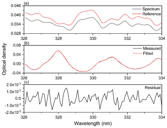
Figure 1.
Typical ozone DOAS fitting from EMI-2 measured on 31 March 2022 at 12:16:11 UTC. (a) Measured spectrum and reference spectrum; (b) measured and fitted ozone optical density; and (c) residuals of the DOAS fitting.
2.3. Iterative AMF Retrieval
The vertical column density (VCD) can be obtained through the ratio of SCD/AMF. Ozone VCD is also called TOC and does not depend on the viewing geometry. The AMFs of the EMI-2 TOC were obtained by multidimensional linear interpolation from a pre-calculated AMF look-up table (LUT) using the radiative transfer model of SCIATRAN [49]. The AMF value is related to the viewing geometry (solar zenith angle (SZA), relative azimuth angle (RAA), and viewing zenith angle (VZA)), surface albedo, ozone a priori profiles, and clouds. The column-dependent climatology profiles from TOMS V8 climatology [50] were used as the ozone a priori profiles, and the parameter node settings are listed in Table 3.
Table 3.
Parameter node settings of the AMF LUT from the EMI-2 TOC.
For partly cloudy EMI-2 ground pixels, AMFs were calculated by the independent pixel approximation (IPA) method [51]. Using the IPA method, the AMFs of partly cloudy ground pixels are determined as the weighted sum of the AMFs from clear and cloudy ground pixels:
where denotes the partly cloudy AMF, denotes the cloud fraction from GOME-2, denotes the cloudy AMF, and denotes the clear-sky AMF. The EMI-2 TOC was then calculated as follows:
where denotes the ozone column, denotes the ozone SCD, and denotes the ozone ghost column (i.e., the quantity below the cloud top height). The ghost column was calculated from the stored LUT of the climatology ozone profiles through multidimensional linear interpolation.
In the EMI TOC retrieval algorithm, TOCs were obtained through a two-step AMF calculation scheme. We noted that the iterative AMF calculation scheme adopted by the EMI-2 was more appropriate. In the iterative AMF calculation scheme, the calculated VCD was used as the ozone column (input to select column-dependent ozone profiles) to calculate the next AMF. This iterative scheme can be expressed as follows:
where denotes the number of iterations. The criterion for stopping the iteration is that the relative deviation between and is less than 0.1%. For most of the EMI-2 pixels, the number of iterations was less than five.
The reference spectrum of EMI was derived from the measured single solar irradiance spectrum from 12 June 2018, which resulted in an obvious stripe effect (Figure 2a). The monthly averaged solar irradiance spectrum was adopted for EMI-2 TOC retrieval, thus substantially decreasing the stripe effect (Figure 2b).
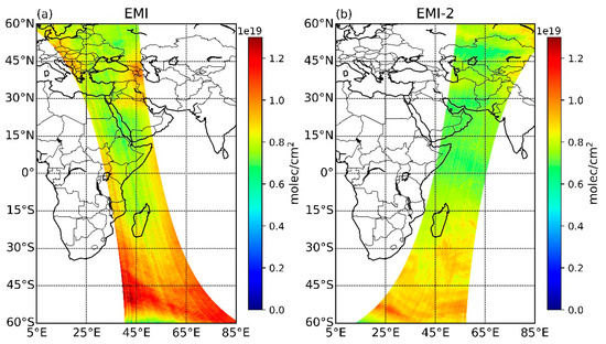
Figure 2.
Example of ozone SCDs showing the (a) obvious stripe effect from EMI (orbit number of 002590) and (b) weak stripe effect from EMI-2 (orbit number of 000813).
3. Results and Discussion
Figure 3 shows an example of global TOCs on 5 November 2021 derived from the EMI-2. In Figure 3, the capacity for monitoring the Antarctic ozone hole (TOC value less than 220 DU, 1 DU = 2.69 1016 molec/cm2) and the daily global coverage are illustrated. In addition, Figure A1 shows a typical application case for monitoring the Antarctic ozone hole through EMI-2 measurements. The time series of averaged Antarctic TOCs (60°S–90°S latitude belts) from EMI-2 is shown in Figure A1, where the blue line at 220 DU denotes the ozone hole threshold.
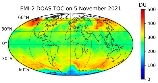
Figure 3.
Global total ozone columns (TOCs) on 5 November 2021, derived from EMI-2.
The monthly averaged TOCs for November 2021 from EMI-2 and TROPOMI are shown in Figure 4, and they have a resampled spatial resolution of 0.25 0.5 (lat lon). The EMI-2 TOCs (Figure 4a) showed global spatial distributions similar to those from TROPOMI (Figure 4b). As shown in Figure 4, the latitude-dependent TOCs and Antarctic ozone hole in November 2021 were monitored. The relative biases of global TOCs between EMI-2 and TROPOMI (Figure 4c) were calculated as follows: .
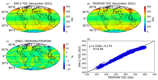
Figure 4.
Spatial distributions of the (a) monthly averaged EMI-2 TOCs, (b) monthly averaged TROPOMI TOCs, (c) averaged relative biases between the EMI-2 TOCs and TROPOMI TOCs, and (d) linear fitting between the EMI-2 TOCs and TROPOMI TOCs in November 2021.
The overall mean relative bias and standard deviation were 0.16% and 2.38%, respectively. The mean relative biases between the EMI-2 and TROPOMI TOCs in the 60°S–90°S, 30°S–60°S, 30°S–30°N, and 30°N–60°N latitude belts were −1.63%, 0.38%, 0.83%, and 0.62%, respectively, with mean standard deviations of 3.56%, 1.55%, 1.36%, and 2.47%, respectively. The mean relative biases were negative near the pole and positive over the tropics, which may have been caused by the differences between Vector Linearized Discrete Ordinate Radiative Transfer (VLIDORT) for TROPOMI TOC calculation and the radiative transfer model of SCIATRAN for EMI-2 TOC calculation. The regression analysis in Figure 4d shows a good correlation between EMI-2 and TROPOMI, with a Pearson correlation coefficient (R) of 0.99. However, the EMI-2 TOCs seemed to be slightly lower than those of TROPOMI when the TOCs were located at a high level. It should be noted that large biases were distributed in the polar area near the coastline, where the surface albedo changed more dramatically owing to the coverage of snow/ice. The surface albedo of the EMI-2 pixel was derived from the OMLER monthly climatology [52], and the effective scene albedo was adopted for the TROPOMI OFFL TOCs. The differences between the climatology albedo and effective scene albedo were less than 0.1 in most of the scenes; however, large differences appeared in the polar area near the coastline in spring [34], which correspond to the large biases in Figure 4c. Therefore, we attribute the large biases (up to 7%) of the polar area near the coastline to the different surface albedo algorithms. In general, the EMI-2 TOCs were in good agreement with those from TROPOMI. In addition, the monthly averaged TOCs for June 2022 from EMI-2 and TROPOMI are shown in Figure A2. In general, EMI-2 TOCs were in good agreement with TROPOMI TOCs, with an overall mean relative bias, standard deviation, and correlation coefficient (R) of 1.28%, 2.79%, and 0.97, respectively. Large negative differences of up to -5% appeared in high latitudes of the northern hemisphere, and positive differences of up to 7% appeared in high latitudes of the southern hemisphere.
Daily reliable TOCs derived from ground-based measurements of the WOUDC dataset were used to validate the EMI-2 TOCs with one year’s data from 1 November 2021 to 31 October 2022. The daily average EMI-2 TOC results were calculated for the ground pixels (0.25° 0.25°) of corresponding ground-based stations. The relative differences between the EMI-2 and ground-based results with respect to the stations’ latitude are shown in Figure 5. As shown in Figure 5, the relative biases between EMI-2 and ground-based TOCs fluctuated from −4.16% to 2.73%, and the mean relative bias and mean standard deviation were 0.70% and 3.65%, respectively. In addition, the latitude-dependent biases appear in Figure 5. EMI TOCs seemed to be lower than the ground-based measurements at high latitudes, which may have been caused by the larger SZAs. The first validations of the EMI-2 DOAS TOCs met the expected accuracy (5%), and we believe that more accurate EMI-2 DOAS TOCs are possible. Detailed station information and the corresponding relative biases are shown in Table 4. Some of the detailed scatter plots between the EMI-2 and ground-based measurements are shown in Figure 6. As shown in Figure 6, the EMI-2 TOCs were in good agreement with the ground-based measurements. However, the EMI-2 TOCs seemed to be higher than ground-based measurements at the Uccle and Haute Provence sites when the TOCs were located at a high level.
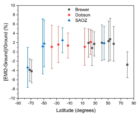
Figure 5.
Relative biases between the EMI-2 and ground-based TOCs.
Table 4.
Detailed station information and corresponding relative biases between the EMI-2 and ground-based TOCs.
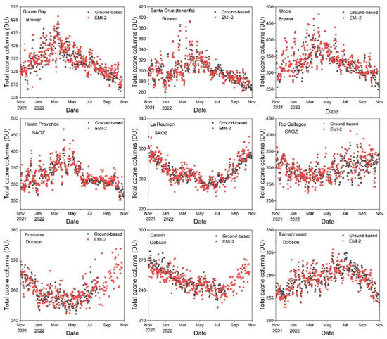
Figure 6.
Scatter plots between the EMI-2 and ground-based TOCs.
4. Conclusions
In this study, the first EMI-2 DOAS TOC results were presented and compared with TROPOMI TOC results. The EMI-2 DOAS TOCs were consistent with the TROPOMI OFFL TOCs, and the overall mean relative bias, mean standard deviation, and correlation coefficient (R) were 0.16%, 2.38%, and 0.99, respectively. The EMI-2 TOC results for November 2021 showed a spatial distribution similar to that of the TROPOMI TOCs. However, large positive differences of up to 7% appeared in some polar areas near the coastline, and negative differences of up to −8% appeared over high latitudes, which were mainly caused by different surface albedo algorithms. In general, the EMI-2 DOAS TOCs were highly consistent with the TROPOMI OFFL TOCs. We selected 20 reliable ground-based measurements distributed at different latitudes from the WOUDC center to evaluate the accuracy of the EMI-2 DOAS TOC results. The relative biases of the selected ground-based stations ranged from −4.16% to 2.73%, and the mean relative biases and standard deviations were 0.70% and 3.65%, respectively, which met the target accuracy (5%). We note that the EMI-2 DOAS TOC results of this research are preliminary, and further improvements should be made to cloud products and surface albedo algorithms. The EMI-2 geometry-dependent surface Lambertian-equivalent reflectivity retrieval should be conducted in the future. In addition, long-term validation at more ground-based stations should be conducted in the future when EMI-2 observations and ground-based measurements from the WOUDC center are available. This study plays an important role in the development of the EMI-2 DOAS TOC product. In the next version of the EMI DOAS TOC algorithm, we hope to achieve a higher accuracy within 3% across different latitudes relative to that of the reliable ground-based measurements from the WOUDC center.
Author Contributions
Conceptualization, Y.Q., F.S. and Y.L.; methodology, Y.Q.; software, Y.Q., H.Z., T.Y. and L.X.; validation, Y.Q. and F.S.; formal analysis, Y.Q. and Y.L.; investigation, Y.Q.; resources, Y.Q., F.S. and Y.L.; writing—original draft preparation, Y.Q.; writing—review and editing, Y.L. and F.S.; visualization, Y.Q.; supervision, Y.L. and F.S.; project administration, F.S.; funding acquisition, F.S. All authors have read and agreed to the published version of the manuscript.
Funding
This research was funded by the National Natural Science Foundation of China (Grant Nos. 41941011 and 41676184) and the Youth Innovation Promotion Association of CAS (Grant No. 2020439).
Data Availability Statement
The data presented in this study are available upon request from the corresponding author.
Acknowledgments
The authors would like to thank the Royal Belgian Institute for Space Aeronomy for providing the QDOAS software and the Institute of Remote Sensing at the University of Bremen for providing the SCIATRAN model. The authors gratefully acknowledge the KNMI/EUMETSAT team for providing the GOME2C cloud product. The authors are also thankful to NASA and WOUDC for providing reliable total ozone column measurements.
Conflicts of Interest
The authors declare no conflict of interest.
Appendix A

Figure A1.
Daily Antarctic TOCs derived from EMI-2 showing the Antarctic ozone holes.

Figure A2.
Spatial distributions of the (a) monthly averaged EMI-2 TOCs, (b) monthly averaged TROPOMI TOCs, (c) averaged relative biases between the EMI-2 TOCs and TROPOMI TOCs, and (d) linear fitting between the EMI-2 TOCs and TROPOMI TOCs in June 2022.
References
- Solomon, S.; Garcia, R.R.; Rowland, F.S.; Wuebbles, D.J. On the depletion of Antarctic ozone. Nature 1986, 321, 755–758. [Google Scholar] [CrossRef]
- Solomon, S. Stratospheric ozone depletion: A review of concepts and history. Rev. Geophys. 1999, 37, 275–316. [Google Scholar] [CrossRef]
- Manney, G.L.; Santee, M.L.; Rex, M.; Livesey, N.J.; Pitts, M.C.; Veefkind, P.; Nash, E.R.; Wohltmann, I.; Lehmann, R.; Froidevaux, L.; et al. Unprecedented Arctic ozone loss in 2011. Nature 2011, 478, 469–475. [Google Scholar] [CrossRef]
- McKenzie, R.L.; Aucamp, P.J.; Bais, A.F.; Björn, L.O.; Ilyas, M.; Madronich, S. Ozone depletion and climate change: Impacts on UV radiation. Photochem. Photobiol. Sci. 2011, 10, 182–198. [Google Scholar] [CrossRef]
- Chipperfield, M.P.; Bekki, S.; Dhomse, S.; Harris, N.R.P.; Hassler, B.; Hossaini, R.; Steinbrecht, W.; Thiéblemont, R.; Weber, M. Detecting recovery of the stratospheric ozone layer. Nature 2017, 549, 211–218. [Google Scholar] [CrossRef]
- Weber, M.; Arosio, C.; Coldewey-Egbers, M.; Fioletov, V.E.; Frith, S.M.; Wild, J.D.; Tourpali, K.; Burrows, J.P.; Loyola, D. Global total ozone recovery trends attributed to ozone-depleting substance (ODS) changes derived from five merged ozone datasets. Atmos. Chem. Phys. 2022, 22, 6843–6859. [Google Scholar] [CrossRef]
- Farman, J.C.; Gardiner, B.G.; Shanklin, J.D. Large losses of total ozone in Antarctica reveal seasonal CIOx/NOx interaction. Nature 1985, 315, 207–210. [Google Scholar] [CrossRef]
- Stolarski, R.S.; Krueger, A.J.; Schoeberl, M.R.; McPeters, R.D.; Newman, P.A.; Alpert, J.C. Nimbus 7 satellite measurements of the springtime Antarctic ozone decrease. Nature 1986, 322, 808–811. [Google Scholar] [CrossRef]
- Grooβ, J.U.; Brautzsch, K.; Pommrich, R.; Solomon, S.; Müller, R. Stratospheric ozone chemistry in the Antarctic: What determines the lowest ozone values reached and their recovery? Atmos. Chem. Phys. 2011, 11, 12217–12226. [Google Scholar] [CrossRef]
- Wohltmann, I.; Lehmann, R.; Rex, M. A quantitative analysis of the reactions involved in stratospheric ozone depletion in the polar vortex core. Atmos. Chem. Phys. 2017, 17, 10535–10563. [Google Scholar] [CrossRef]
- Keeble, J.; Braesicke, P.; Abraham, N.L.; Roscoe, H.K.; Pyle, J.A. The impact of polar stratospheric ozone loss on southern hemisphere stratospheric circulation and climate. Atmos. Chem. Phys. 2014, 14, 18049–18082. [Google Scholar] [CrossRef]
- Velders, G.J.M.; Ravishankara, A.R.; Miller, M.K.; Molina, M.J.; Alcamo, J.; Daniel, J.S.; Fahey, D.W.; Montzka, S.A.; Reimann, S. Preserving Montreal Protocol climate benefits by limiting HFCs. Science 2012, 335, 922–923. [Google Scholar] [CrossRef] [PubMed]
- Chipperfield, M.P.; Dhomse, S.S.; Feng, W.; McKenzie, R.; Velders, G.J.; Pyle, J.A. Quantifying the ozone and ultraviolet benefits already achieved by the Montreal Protocol. Nat. Commun. 2015, 6, 7233. [Google Scholar] [CrossRef]
- Goyal, R.; England, M.H.; Gupta, A.S.; Jucker, M. Reduction in surface climate change achieved by the 1987 Montreal Protocol. Environ. Res. Lett. 2019, 14, 124021. [Google Scholar] [CrossRef]
- Banerjee, A.; Fyfe, J.C.; Polvani, L.M.; Waugh, D.; Chang, K.L. A pause in southern hemisphere circulation trends due to the Montreal Protocol. Nature 2020, 579, 544–548. [Google Scholar] [CrossRef]
- Kerr, R.A. First detection of ozone hole recovery claimed. Science 2011, 332, 160. [Google Scholar] [CrossRef]
- Solomon, S.; Lvy, D.J.; Kinnison, D.; Mills, M.J.; Neel, R.R.; Schmidt, A. Emergence of healing in the Antarctic ozone layer. Science 2016, 353, 269–274. [Google Scholar] [CrossRef]
- Heath, D.F.; Krueger, A.J.; Roeder, H.A.; Henderson, B.D. The solar backscatter ultraviolet and total ozone mapping spectrometer (SBUV/TOMS) for Nimbus G. Opt. Eng. 1975, 14, 323–331. [Google Scholar] [CrossRef]
- Bhartia, P.K.; McPeters, R.D.; Flynn, L.E.; Taylor, S.; Kramarova, N.A.; Frith, S.; Fisher, B.; DeLand, M. Solar Backscatter UV (SBUV) total ozone and profile algorithm. Atmos. Meas. Tech. 2013, 6, 2533–2548. [Google Scholar] [CrossRef]
- Kuttippurath, J.; Nair, P.J. The signs of Antarctic ozone hole recovery. Sci. Rep. 2017, 7, 585. [Google Scholar] [CrossRef]
- Weber, M.; Arosio, C.; Feng, W.H.; Dhomse, S.S.; Chipperfield, M.P.; Meier, A.; Burrows, J.P.; Eichmann, K.U.; Richter, A.; Rozanov, A. The unusual stratospheric Arctic winter 2019/20: Chemical ozone loss from satellite observations and TOMCAT chemical transport model. J. Geophys. Res. 2021, 126, e2020JD034386. [Google Scholar] [CrossRef]
- Verstraeten, W.W.; Neu, J.L.; Williams, J.E.; Bowman, K.W.; Worden, J.R.; Boersma, K.F. Rapid increases in tropospheric ozone production and export from China. Nat. Geosci. 2015, 8, 690–695. [Google Scholar] [CrossRef]
- Kuttippurath, J.; Godin-Beekmann, S.; Lefèvre, F.; Nikulin, G.; Santee, M.L.; Froidevaux, L. Record-breaking ozone loss in the Arctic winter 2010/2011: Comparison with 1996/1997. Atmos. Chem. Phys. 2012, 12, 7073–7085. [Google Scholar] [CrossRef]
- Solomon, S.; Kinnison, D.; Bandoro, J.; Garcia, R. Simulation of polar ozone depletion: An update. J. Geophys. Res. Atnos. 2015, 120, 7958–7974. [Google Scholar] [CrossRef]
- Grooß, J.U.; Müller, R. Simulation of record Arctic stratospheric ozone depletion in 2020. J. Geophys. Res. Atmos. 2021, 126, e2020JD033339. [Google Scholar] [CrossRef]
- Weber, M.; Burrows, J.P.; Cebula, R.P. GOME solar UV/VIS irradiance measurements between 1995 and 1997–first results on proxy solar activity studies. Sol. Phys. 1998, 177, 63–77. [Google Scholar] [CrossRef]
- Burrows, J.P.; Weber, M.; Buchwitz, M.; Rozanov, V.; Ladstätter-Weißenmayer, A.; Richter, A.; DeBeek, R.; Hoogen, R.; Bramstedt, K.; Eichmann, K.U.; et al. The global ozone monitoring experiment (GOME): Mission concept and first scientific results. J. Atmos. Sci. 1999, 56, 151–175. Available online: https://journals.ametsoc.org/view/journals/atsc/56/2/1520-0469_1999_056_0151_tgomeg_2.0.co_2.xml (accessed on 1 March 2023). [CrossRef]
- Thomas, W.; Hegels, E.; Slijkhuis, S.; Spurr, R.; Chance, K. Detection of biomass burning combustion products in Southeast Asia from backscatter data taken by the GOME spectrometer. Geophys. Res. Lett. 1998, 25, 1317–1320. [Google Scholar] [CrossRef]
- Loyola, D.G.; Coldewey-Egbers, R.M.; Dameris, M.; Garny, H.; Stenke, A.; van Roozendael, M.; Lerot, C.; Balis, D.; Koukouli, M. Global long-term monitoring of the ozone layer—A prerequisite for predictions. Int. J. Remote Sens. 2009, 30, 4295–4318. [Google Scholar] [CrossRef]
- Loyola, D.G.; Koukouli, M.E.; Valks, P.; Bails, D.S.; Hao, N.; Van Roozendael, M.; Spurr, R.J.D.; Zimmer, W.; Kiemle, S.; Lerot, C.; et al. The GOME-2 total column ozone product: Retrieval algorithm and ground-based validation. J. Geophys. Res. 2011, 116, D07302. [Google Scholar] [CrossRef]
- Hao, N.; Koukouli, M.; Inness, A.; Valks, P.; Loyola, D.; Zimmer, W.; Balis, D.; Zyrichidou, I.; Van Roozendael, M.; Lerot, C. GOME-2 total ozone columns from MetOp-A/MetOp-B and assimilation in the MACC system. Atmos. Meas. Tech. 2014, 7, 2937–2951. [Google Scholar] [CrossRef]
- Veefkind, J.P.; de Han, J.F.; Brinksma, E.J.; Kroon, M.; Levelt, P.F. Total ozone from the ozone monitoring instrument (OMI) using the DOAS technique. IEEE. Trans. Geosci. Remote Sens. 2006, 44, 1239–1244. [Google Scholar] [CrossRef]
- Veefkind, J.P.; Aben, I.; McMullan, K.; Förster, H.; de Vries, J.; Otter, G.; Claas, J.; Eskes, H.J.; de Haan, J.F.; Kleipool, Q.; et al. TROPOMI on the ESA Sentinel-5 Precursor: A GMES mission for global observations of the atmospheric composition for climate, air quality and ozone layer applications. Remote Sens. Environ. 2012, 120, 70–83. [Google Scholar] [CrossRef]
- Garane, K.; Koukouli, M.E.; Verhoelst, T.; Lerot, C.; Heue, K.P.; Fioletov, V.; Balis, D.; Bais, A.; Bazureau, A.; Dehn, A.; et al. TROPOMI/S5P total ozone column data: Global ground-based validation and consistency with other satellite missions. Atmos. Meas. Tech. 2019, 12, 5263–5287. [Google Scholar] [CrossRef]
- Cheng, L.X.; Tao, J.H.; Valks, P.; Yu, C.; Liu, S.; Wang, Y.P.; Xiong, X.Z.; Wang, Z.F.; Chen, L.F. NO2 retrieval from the environmental trace gases monitoring instrument (EMI): Preliminary results and intercomparison with OMI and TROPOMI. Remote Sens. 2019, 11, 3017. [Google Scholar] [CrossRef]
- Zhang, C.X.; Liu, C.; Chan, K.L.; Hu, Q.H.; Liu, H.R.; Li, B.; Xing, C.Z.; Tan, W.; Zhou, H.J.; Si, F.Q.; et al. First observation of tropospheric nitrogen dioxide from the environmental trace gases monitoring instrument onboard the Gaofen-5 satellite. Light Sci. Appl. 2020, 9, 66. [Google Scholar] [CrossRef]
- Zhao, M.J.; Si, F.Q.; Wang, Y.; Zhou, H.J.; Wang, S.M.; Jiang, Y.; Liu, W.Q. First year on-orbit calibration of the Chineses environmental trace gases monitoring instrument onboard the gaofen-5. IEEE. Trans. Geosci. Remote Sens. 2020, 58, 8531–8540. [Google Scholar] [CrossRef]
- Qian, Y.Y.; Luo, Y.H.; Si, F.Q.; Zhou, H.J.; Yang, T.P.; Yang, D.S.; Xi, L. Total ozone columns from the environmental trace gases monitoring instrument (EMI) using the DOAS method. Remote Sens. 2021, 13, 2098. [Google Scholar] [CrossRef]
- Puķīte, J.; Wagner, T. Quantification and parametrization of non-linearity effects by higher-order sensitivity terms in scattered light differential optical absorption spectroscopy. Atmos. Meas. Tech. 2016, 9, 2147–2177. [Google Scholar] [CrossRef]
- Zhao, M.J.; Si, F.Q.; Zhou, H.J.; Jiang, Y.; Ji, C.Y.; Wang, S.M.; Zhan, K.; Liu, W.Q. Pre-launch radiometric characterization of EMI-2 on the gaofen-5 series of satellites. Remote Sens. 2021, 13, 2843. [Google Scholar] [CrossRef]
- Platt, U.; Stutz, J. Differential Optical Absorption Spectroscopy: Principles and Applications; Springer: Berlin/Heidelberg, Germany, 2008. [Google Scholar]
- Wang, P.; Stammes, P.; van der A, R.; Pinardi, G.; van Roozendael, M. FRESCO+: An improved O2 A-band cloud retrieval algorithm for tropospheric trace gas retrievals. Atmos. Chems. Phys. 2008, 8, 6565–6576. [Google Scholar] [CrossRef]
- Danckaert, T.; Fayt, C.; van Roozendael, M.; Smedt, I.D.; Letocart, V.; Merlaud, A.; Pinardi, G. QDOAS Software User Manual. Available online: https://uv-vis.aeronomie.be/software/QDOAS/QDOAS_manual.pdf (accessed on 20 October 2020).
- Bogumil, K.; Orphal, J.; Homann, T.; Voigt, S.; Spietz, P.; Fleischmann, O.C.; Vogel, A.; Hartmann, M.; Kromming, H.; Bovensman, H.; et al. Measurements of molecular absorption spectra with the SCIAMACHY preflight model: Instrument characterization and reference data for atmospheric remote-sensing in the 230–2380 nm region. J. Photochem. Photobiol. A-Chem. 2003, 157, 167–184. [Google Scholar] [CrossRef]
- Vandaele, A.C.; Hermans, C.; Simon, P.C.; Roozendael, M.V.; Guilmot, J.M.; Carleer, M.; Colin, R. Fourier transform measurement of NO2 absorption cross-section in the visible range at room temperature. J. Atmos. Chem. 1996, 25, 289–305. [Google Scholar] [CrossRef]
- Vandaele, A.C.; Hermans, C.; Fally, S. Fourier transform measurements of SO2 absorption cross sections: II.: Temperature dependence in the 29,000–44,000 cm−1 (227–345 nm) region. J. Quant. Spectrosc. Radiat. Transf. 2009, 110, 2115–2126. [Google Scholar] [CrossRef]
- Fleischmann, O.C.; Hartmann, M. New ultraviolet absorption cross-sections of BrO at atmospheric temperatures measured by time-windowing Fourier transform spectroscopy. J. Photochem. Photobiol. A Chem. 2004, 168, 117–132. [Google Scholar] [CrossRef]
- Meller, R.; Moortgat, G.K. Temperature dependence of the absorption cross sections of formaldehyde between 223 and 323 K in the wavelength range 225–375 nm. J. Geophys. Res. 2000, 105, 7089–7101. [Google Scholar] [CrossRef]
- Rozanov, V.V.; Rozanov, A.V.; Kokhanovsky, A.A.; Burrows, J.P. Radiative transfer through terrestrial atmosphere and ocean: Software package SCIATRAN. J. Quant. Spectrosc. Radiat. Transf. 2014, 133, 13–71. [Google Scholar] [CrossRef]
- Wellemeyer, C.G.; Bhartia, P.K.; Taylor, S.L.; Qin, W.; Ahn, C. Version 8 total ozone mapping spectrometer (TOMS) algorithm. Quadrenn. Ozone Symp. 2004, 1, 635–636. [Google Scholar]
- Vardhan, H.; Wielicki, B.A.; Ginger, K.M. The interpretation of remotely sensed cloud properties from a model parameterization perspective. J. Clim. 1994, 7, 1987–1998. Available online: http://www.jstor.org/stable/26198681 (accessed on 1 March 2023). [CrossRef]
- Kleipool, Q.L.; Dobber, M.R.; de Haan, J.F.; Levelt, P.E. Earth surface reflectance climatology from 3 years of OMI data. J. Geophys. Res. Atmos. 2008, 113, D18308. [Google Scholar] [CrossRef]
Disclaimer/Publisher’s Note: The statements, opinions and data contained in all publications are solely those of the individual author(s) and contributor(s) and not of MDPI and/or the editor(s). MDPI and/or the editor(s) disclaim responsibility for any injury to people or property resulting from any ideas, methods, instructions or products referred to in the content. |
© 2023 by the authors. Licensee MDPI, Basel, Switzerland. This article is an open access article distributed under the terms and conditions of the Creative Commons Attribution (CC BY) license (https://creativecommons.org/licenses/by/4.0/).