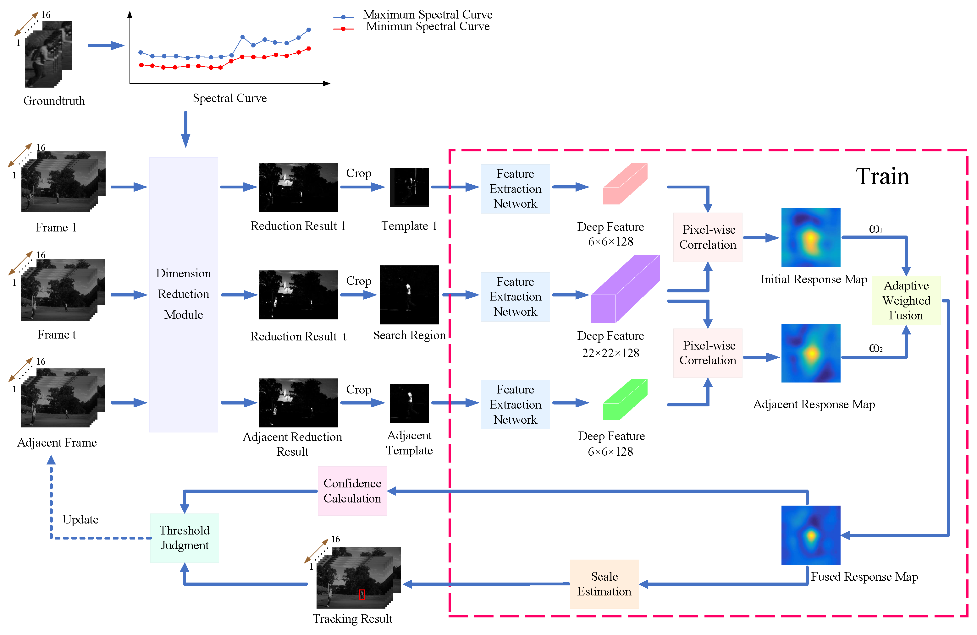
Article

Hyperspectral Video Tracker Based on Spectral Deviation Reduction and a Double Siamese Network

1
School of Physics, Xidian University, Xi’an 710071, China
2
School of Electronics and Information Engineering, Wuxi University, Wuxi 214105, China
3
School of Electronics and Information Engineering, Nanjing University of Information Science and Technology, Nanjing 210044, China
4
Computer Science and Engineering Group, Indian Institute of Information Technology, Sri City 441108, India
5
School of Artificial Intelligence and Computer, Jiangnan University, Wuxi 214122, China
*
Author to whom correspondence should be addressed.
Remote Sens. 2023, 15(6), 1579; https://doi.org/10.3390/rs15061579
Submission received: 2 March 2023 / Revised: 9 March 2023 / Accepted: 10 March 2023 / Published: 14 March 2023
(This article belongs to the Special Issue Hyperspectral Object Tracking)

Abstract

:
The advent of hyperspectral cameras has popularized the study of hyperspectral video trackers. Although hyperspectral images can better distinguish the targets compared to their RGB counterparts, the occlusion and rotation of the target affect the effectiveness of the target. For instance, occlusion obscures the target, reducing the tracking accuracy and even causing tracking failure. In this regard, this paper proposes a novel hyperspectral video tracker where the double Siamese network (D-Siam) forms the basis of the framework. Moreover, AlexNet serves as the backbone of D-Siam. The current study also adopts a novel spectral–deviation-based dimensionality reduction approach on the learned features to match the input requirements of the AlexNet. It should be noted that the proposed dimensionality reduction method increases the distinction between the target and background. The two response maps, namely the initial response map and the adjacent response map, obtained using the D-Siam network, were fused using an adaptive weight estimation strategy. Finally, a confidence judgment module is proposed to regulate the update for the whole framework. A comparative analysis of the proposed approach with state-of-the-art trackers and an extensive ablation study were conducted on a publicly available benchmark hyperspectral dataset. The results show that the proposed tracker outperforms the existing state-of-the-art approaches against most of the challenges.

1. Introduction

Recently, machine learning-based target tracking [1,2] has become an important frontier in the field of computer vision, with applications in different fields [3,4], such as autonomous driving, aerospace, robotic navigation, and sports broadcasting. Most of the target tracking algorithms use the characteristics of the target, in the initial frames of a sequence, to predict the position of the target in the subsequent frames. However, various factors, including illumination variance, environmental changes, occlusion, etc., may alter the appearance of the target between the subsequent frames, causing tracking failure. Hence, it is important to design an appropriate target tracking model to adapt to the complex and changing environments to achieve tracking robustness. Recently, the development of hyperspectral imaging equipment with a high frame rate has popularized the hyperspectral videos (HSVs) for effective target tracking. In comparison to the RGB images [5], the hyperspectral images (HSIs) [6,7,8] pose the spatial and spectral information to improve the descriptive dimension of the target. The similar colored targets and backgrounds, which are indistinguishable in the RGB images, can be distinguished in the HSIs. This is because the HSIs use the spectral reflectance of the targets and backgrounds over tens to thousands of wavebands.
In comparison to RGB image-based trackers, hyperspectral video-based trackers not only use the features of the target in the spatial direction but also in the spectral direction. In the design of trackers, hyperspectral video-based trackers give more emphasis on making full use of spectral information. Xiong et al. [9] proposed a material-based HSV tracking algorithm that uses the material features and spherical coordinate system to combine the two-dimensional spatial [10] and one-dimensional spectral histogram of oriented gradients (HOG). However, in such approaches, it is difficult to ensure tracking robustness due to the limitations of the material library. Zhao et al. [11] fused the features, extracted using the residual network (ResNet) [12] and three-dimensional linear spatial scale theory [13], to robustly track the target. However, this method requires too many parameters and is highly complex, resulting in the drifting of the target. Although Chen et al. [14] combined different spectral filters for spatial-spectral feature extraction, the approach did not consider the interference of the target analogs during tracking. Liu et al. [15] used two independent branches to extract spatial features and spectral features, respectively, which solved the problem of small-sample learning. Later, Liu et al. [16] introduced a spatial–spectral cross-attention module to fuse the spatial and spectral features extracted from a RGB-based tracker. However, these algorithms required a change in the number of network channels and the retraining of the network.
In this research, to overcome the above-discussed problems, we adopt a fully-convolutional Siamese network (SiamFC) [17] as the basic framework, and propose a hyperspectral video tracker based on spectral deviation reduction and double Siamese network (SD-HVT). The proposed tracker framework constitutes of four modules, namely dimensionality reduction, feature extraction, matching, and the regression modules. The dimensionality reduction module transforms the original HSIs to single-channel images, which are then fed to the feature extraction network. This research proposes a novel dimensionality reduction method that adopts spectral deviation (DRSD) to effectively resolve the illumination variations and to improve the background/target discrimination in the transformed space. The feature extraction module obtains the characteristic features to distinguish the target from the background. This research proposes a novel double Siamese network (D-Siam) that generates an adjacent template based on the original. Finally, the matching module is used to locate the target, and the regression module could adapt to the scale variations of the target. It should be noted that adaptive weights are employed in the matching module to fuse the two representations yielded by the D-Siam to precisely locate the target. The regression module adopts the traditional multiscale computation. To evaluate the performance of the proposed SD-HVT, a series of real HSVs, discussed in [9], are used.
The four key contributions of the paper are summarized as follows:
  • A novel dimensionality reduction method, named DRSD, is proposed for HSIs. The maximum and minimum spectral curves of the target in the first frame are used to screen the spectral curves of the search area, and the spectral deviation between them is used to reduce the spectral dimension. This method can enhance the tracked target in advance and suppress the background. Compared with the traditional methods, the proposed method can enhance the tracked target in advance and suppress the background, which is helpful to the subsequent feature extraction.
  • A novel framework, named D-Siam, is designed to use the initial and adjacent frames to accurately locate the target. In comparison to the original SiamFC, D-Siam has higher accuracy and can better adapt to the changes in the appearance of the target in motion. The D-Siam separates the template update process from the original template, thereby reducing template contamination as compared to the traditional linear update methods.
  • A new weighted fusion method is proposed for dual response map fusion, which automatically corrects the weights according to the changes of the target in the sequence. Hence, the approach provides better robustness for target tracking as compared to the existing state-of-the-art approaches.
  • In order to judge whether the tracked results are reliable, a confidence judgment module is set to effectively reduce the impact of excessive changes on subsequent tracking.
The remaining portions of this manuscript are organized as follows. Section 2 presents a summary of the research related to hyperspectral target tracking. In Section 3, the framework and background rationale of the proposed algorithm are presented in detail. Section 4 presents the experimental results of the proposed and other benchmark approaches on the given hyperspectral sequences. Finally, conclusions are drawn in Section 5.

2. Related Works

In this section, we briefly discuss the research related to the three key modules of the proposed HSV-based target tracker, namely, the dimensionality reduction, target tracking, and template update.
Dimensionality Reduction. Among the different dimensionality reduction techniques, the feature extraction-based approaches compute an optimal projection matrix to reduce the dimension. On the other hand, the band selection-based dimensionality reduction techniques select the most representative bands from the original bands. The feature selection methods [18,19] are prone to lose the relevant spectral information as compared to the feature extraction approaches. The principal component analysis (PCA) [20,21], the most commonly used feature extraction approach, adopts a linear projection to map the high dimensional data into a lower dimensional space, using fewer dimensions of the data while retaining more of the original data points. In a similar work based on PCA, Green et al. [22] proposed the maximum noise fraction approach, which adopted cascaded PCA transformations to consider the noisy nature of the hyperspectral spectra. In a similar research, Xia et al. [23] proposed kernelized PCA, which employed PCA after transforming the original nonlinear data to a linear higher dimensional space. Unlike the PCA-based approaches, Villa et al. [24] proposed the independent component analysis for hyperspectral image analysis, which transformed the data into separate components and employed fewer components to describe the data. Although the above-discussed approaches transform the data based on the data distribution, they ignore the class labels of the data. In this regard, linear discriminant analysis (LDA) [25] was proposed to transform the data points into a latent space where the different classes are distinguishable. Similarly, locally linear embedding (LLE) [26] is a non-linear dimensionality reduction algorithm that preserves the original stream structure. The Laplacian Eigenmap (LE) [27] is similar to the LLE algorithm, due to the reason that the relationships between data are constructed from a local perspective. Although Nielsen et al. [28] proposed the maximum autocorrelation factor for feature extraction, the approach yielded poor performance for the hyperspectral data. In order to improve the accuracy of hyperspectral data classification, Li et al. [29] proposed a sparse penalty regularised linear discriminant method for dimensionality reduction, which yielded good classification results on benchmark hyperspectral data sets. Huang et al. [30] proposed a spatial–spectral popular reconstruction to preserve embedding. The unsupervised dimensionality reduction method for classifying hyperspectral images is able to reduce the effect of noise and reconstruct the weights. However, the algorithm is complex and takes a long time to compute. Hong et al. [31] proposed a joint asymptotic subspace analysis that could maintain a similar topology between the compressed and original data. This method is used in the treatment of spectral variability.
Target Tracking. The tracking algorithm, proposed in the current study, is related to mainly two classes of tracking algorithms, namely the correlation filtering-based [1,2,32,33,34,35] and Siamese network-based trackers [17,36,37,38,39]. Among the correlation filtering-based trackers, Bolme et al. [1] employed the sum of the minimum output squared error (MOSSE) filter, which used raw gray-scale features. However, the approach did not take into account the variations in the target scale and frequently lost the target in adverse conditions. In order to overcome the limitations of the gray-scale features, Henriques et al. [2] proposed kernelized correlation filters (KCFs), which used HOG features [10] to replace the gray-scale features. This type of algorithm relied on a circular matrix and did not give satisfactory results for multi-scale target tracking. Danelljan et al. [40] proposed the spatial regularization discriminant correlation filter (SRDCF), which used a large detection region, in addition to employing the filter coefficients for null regularization and penalizing the boundary regions. However, this approach resulted in increased computational complexity and lowered the processing speed. In this direction, Bertinetto et al. [41] used two complementary features, the HOG and color features, for modeling the target. The tracking results are then fused to improve the tracking performance. Li et al. [42] proposed a spatiotemporal Regularised Correlation Filter, which can adapt well to large changes in the appearance of the target. Nowadays, with the advent of deep learning, deep features are being widely used instead of hand-crafted features. In this regard, Song et al. [43] employed deep features, derived from ResNet, for target tracking to achieve better robustness as compared to the use of conventional hand-crafted features.
Unlike the deep neural networks used in the correlation filtering-based trackers, Siamese networks realize end-to-end trainability for the first time. Bertinetto et al. [17] proposed SiamFC, an end-to-end tracking network, which used two fully convolutional concatenated networks for target tracking, with both networks sharing the same weights. Similarly, Bo et al. [36] proposed the Siamese region proposal network (SiamRPN) that did not perform similarity calculations but selected the final target based on regression bias and classification scores. The class imbalance problem in the training samples generally limits the performance of the tracking algorithms. In order to solve the problem that only relatively shallow convolutional networks can be used for conjoined network-based trackers, the SiamRPN++ network [39] adopted a position-balancing sampling to alleviate the position bias problem during training. The network framework, proposed in our current study, uses both initial and adjacent frames to fully localize the target, which offers higher accuracy and better adaptation to the changes in the targets in motion. Wang et al. [44] first used the transformer model for target tracking. The authors constructed two branches of the transformer encoder and transformer decoder to create high-quality target tracking templates by using the attention-based features and efficient contextual information utilization of the transformer model. In order to obtain more contextual information for images, Lin et al. [45] used the structure of convolutional neural networks to improve the traditional transformer model by using shifted windows to better match the image information.
Moreover, to adapt to the changes in the size of the target during the tracking process, the scale estimation module also plays an important role. Li et al. [46] proposed the fusion of color names [47] and fast histograms of oriented gradient [48] features using a scale adaptive multiple feature algorithm. The approach employed a pool of scale factors to sample multiple image blocks of different scales. In this direction, Danelljan et al. [32] proposed discriminative scale space tracking (DSST), which used a scale estimation module along with the KCF to achieve scale adaptation. Inspired by the module independence, the region proposal network (RPN) [36,39] was used as a scale estimation module for the existing tracking frameworks. In addition, the refinement module [49,50] was also utilized to replace the RPN in recent years to achieve better results.
Template update. Template update is also a key issue in the tracking algorithms. The simple linear update [2,51] is the generally adopted update method. However, the existing update methods are unreliable when the appearance of the target changes. To resolve this problem, Danelljan et al. [52] focused more on the recent frames rather than on the historical frames. Danelljan et al. [53] divided the training samples into different subsets where each of these subsets represented a distinct appearance. In recent years, researchers [54,55,56] have employed online learning strategies to update the template. However, these methods failed to effectively model the target when the shape of the target drastically changes. Therefore, we use two templates to achieve the tracking task, namely initial template and adjacent templates. The initial template is not updated to ensure tracking accuracy, and the adjacent template is fully updated to adapt to the changes in the appearance of the target.

3. Proposed Algorithm

This section discusses the details of the proposed algorithm. The overall framework of the proposed algorithm is presented in Figure 1.
In the proposed framework, the ground truth is first used to extract two spectral curves, namely the maximum spectral curve (MASC) and the minimum spectral curve (MISC). Both of these two curves are used to judge the possible range of the target spectral curve, considering the influence of the light. Then, the dimensionality of the original HSIs is reduced by computing the deviation between the target spectral curve and the spectral range from MISC to MASC. Subsequently, the D-Siam framework is employed to simultaneously compute the similarities of the search region with template 1 and the adjacent template. These two results, namely the initial response map and the adjacent response map, are obtained through feature extraction network and pixel-wise correlation. Further, an adaptive-weight-based fusion is utilized to fuse these two response maps to obtain the fused response map. Finally, the target scale is estimated by comparing several fused response maps generated by different scale search regions. In addition, confidence calculation module obtains the confidence of the predicted target, which is used to decide whether to update the adjacent template in the threshold judgment module. In Section 3.1, the proposed spectral deviation-based dimensionality reduction method is introduced in detail. The SiamFC framework, adopted as a base framework in this study, is briefly discussed in Section 3.2. In Section 3.3, the proposed D-Siam framework and the target prediction approach are discussed, including weighted fusion and scale estimation. Moreover, then, the threshold judgment method is discussed in Section 3.4. Finally, the pseudocode of the proposed algorithm is given in Section 3.5.

3.1. Dimensionality Reduction Based on Spectral Deviation

To simplify the processing flow of the subsequent D-Siam module, we propose a dimensionality reduction method based on the spectral deviation to reduce the input dimensions and improve the separability between the target and background.
Initially, two spectral curves are extracted from the local area in the ground truth of the first frame, namely MASC and MISC. The ground truth is regarded as the real location of the target, which is provided along with the tracking sequences. However, due to the irregular nature of the target and the fact that the ground truth is a regular rectangle box, there can be some background pixels in the ground truth. Therefore, the local area, a small square area with size h × h at the center of ground truth, is used to represent the target pixels. It may be noted that a large-sized local area may include the background pixels, while a small-sized one will cause errors. Empirically, h is set to 3, hence, L R 3 × 3 × B represents the local area of the target at the first frame, where B is the number of bands and is 16 for the dataset [9] in the current study.
The spectral curves of all pixel points in L are counted, and the MASC and MISC are obtained by counting the maximum and minimum values in each band. The ground truth and these two spectral curves are shown in Figure 2.
In order to minimize the effect of illumination variations on the dimensionality reduction and subsequent target tracking, the original hyperspectral image I i n R H i n × W i n × B is de-averaged as:
C i = C i b C i b = I i b i n mean ( I i i n ) i 1 , . . . , H i n × W i n , b 1 , . . . , B
where C i is the de-averaged spectral curve of the i-th pixel, C i b represents the value in b-th band of C i and I i b i n is the value of i-th pixel in b-th band of I i n ; H i n and W i n are the height and width of the original hyperspectral image, respectively. mean ( · ) represents the average function, which is calculated as
mean I i i n = 1 B × b = 1 B I i b i n
After obtaining the spectral curve of each pixel C i , the spectral deviation of C i and the spectral range bound by MASC and MISC are calculated. This is used to estimate the difference between C i and the spectral curve of the target. The spectral deviation of each band is computed as
D i b = ( C i b C m a x b ) × ( C i b C m i n b ) ( C m a x b + C m i n b ) 2
where D i b represents the spectral deviation value of the i-th pixel in the b-th band, C i b is the b-th band of C i , and C m a x b . Moreover, C m i n b represent the pixel values of MASC and MISC in the b-th band, respectively.
However, in practice, a deviation value D i b of zero means there is no difference between C i and the spectral curve of the target in the b-th band, while a negative deviation value also means the same. Therefore, D i b is quantified as Q i b .
Q i b = 0 if D i b 0 D i b otherwise
where Q i b is the quantitative deviation of D i b . All negative values are set to 0, and the total deviation of each pixel Q i can be obtained by summing Q i b in spectral direction as:
Q i = b = 1 B Q i b
The dimensionality reduction is performed based on the total deviation degree of each pixel as:
I r = I i r I i r = 0 if Q i > T 1 Q i T otherwise
where I r denotes the result of the dimensionality reduction, I i r is the i-th pixel of I r , and T is the segmentation threshold. The larger the value of T, the wider the deviation range contained in I r , and the less obvious the target. Empirically, the value of T is set to half of Q m a x , and Q m a x is the maximum value among all Q i .
It should be noted that the range of the values of I r is from 0 to 1. However, to meet the requirement of the subsequent D-Siam network, the values of I r are mapped to a range from 0 to 255 as:
I f = round I r 255
where round ( · ) denotes the rounding operation, and I f is the dimensionality reduced image after mapping. One of the original hyperspectral images and the corresponding dimensionality reduction results are shown in Figure 3.
It can be seen from Figure 3 that the image data volume of the dimensionality reduction result becomes one-sixteenth of the original hyperspectral image in this experiment. As a result, the data involved in the calculation has been reduced to one-sixteenth of the original amount, leading to a corresponding reduction in computational cost. Moreover, compared with the result of PCA, the result of the proposed DRSD method can better suppress the background and highlight the target.

3.2. Fully Convolutional Siamese Network

Fully convolutional Siamese network (SiamFC) consists of two sub-networks with the same structure. The inputs to the Siamese network, considered in this study, are two images, one is the template while the other is the search region. The template and the search region are selected from the first and the subsequent frames of the sequence, respectively. Each sub-network processes an image and uses the forward passes independently to generate the feature maps of the template and the search region. Subsequently, the cross-correlation computation is performed using the similarity measurement function on the two feature maps to yield a score map. Finally, the upsampling operation is performed on the score map to transform it to the response map. The point with the highest value in the response map is considered to be the center point of the object to be tracked in the subsequent frames. The overall framework of the SiamFC is shown in Figure 4. Although SiamFC has a significant improvement in real-time performance and accuracy, as Compared to the previous trackers, it is still limited in its ability to handle significant changes in the appearance of the target being tracked.

3.3. Double-Siamese Network

The proposed D-Siam framework can be considered an improved version of the SiamFC framework. On the basis of the comparison with the initial template, an additional comparison with the adjacent template is also implemented. Therefore, unlike SiamFC, the input of D-Siam is a group of three images, namely the template 1 z 1 R 127 × 127 × 3 , the adjacent template z a R 127 × 127 × 3 and the search region x R 255 × 255 × 3 . All three images are, respectively, obtained from frame 1 I 1 R H i n × W i n × B , the frame t I t R H i n × W i n × B , and the adjacent frame I a R H i n × W i n × B . These three images are dimensionality reduced using Equations (1)–(7), discussed in Section 3.1, to obtain the reduction result 1 E 1 R H i n × W i n × 1 , the reduction result t E t R H i n × W i n × 1 and the adjacent reduction result E a R H i n × W i n × 1 , respectively. As the dimensionality-reduced images are single-channel images with the same size, they are cropped to the specific size and are replicated three times to form the three-channel images. Similar to SiamFC, AlexNet is also used as the backbone of D-Siam, and the network weights are shared in all three networks. It should be noted that the processing using AlexNet yields two response maps. One is the initial response map R i R 272 × 272 × 1 , which is obtained by calculating the latent space similarity between the initial template and the search region. Another response map, named the adjacent response map R a R 272 × 272 × 1 , is also obtained using similar calculations between the adjacent template and the search region. A group of the initial response map and the adjacent response maps generated in the current experiments are shown in Figure 5.
As is evident from Figure 5, the peak area of the adjacent response map is more concentrated than that of the initial response map. This is because the search region is more similar to the adjacent template as compared to the initial template. However, the initial template is also important to prevent tracking drift. Therefore, to obtain a more robust tracking result, two response maps are fused with adaptive weights. As mentioned in [35], the peak side lobe ratio (PSLR) of the response map is usually used to evaluate the confidence of the final response map. However, considering the characteristic differences between the two templates, the PSLR of each response map is further modified as:
ω i = F p R i × t 2 t 1
ω a = F p R a × F c t a
where ω i and ω a are the weights of R i and R a , respectively. Moreover, t is the frame index, and the constant 2 in Equation (8) is used to limit the range of t 2 t 1 to less than 1. The F c ( · ) is the confidence calculation function, which will be introduced in Section 3.4. Moreover, t a denotes the frame index of the adjacent frame, and it should be noted that t a is smaller than t. Therefore, F c t a is a value calculated in advance. However, for special cases, ω a is set to be the same as ω i for the first frame to be tracked. In addition, F p ( · ) is the function for computing PSLR and is given as:
F p x = υ x m a x υ x m e a n σ x
where υ x m a x is the maximum value of x, υ x m e a n denotes the average value of x, and σ x is the standard deviation of x.
Additionally, to limit the range of the fused response map, ω i and ω a are normalized to ω 1 and ω 2 . Finally, the fused response map is calculated using ω 1 and ω 2 , and the fused result of the two response maps is shown in Figure 6.
R f = ω 1 × R i + ω 2 × R a
ω 1 = ω i ω i + ω a
ω 2 = ω a ω i + ω a
where R f denotes the fused response map, and ω 1 and ω 2 are the normalized weights.
It can be seen from Figure 6 that the fused response map is more similar to the adjacent response map. Moreover, the fused response map has a more small peak area compared with the other two maps, which leads to a higher PSLR and a more robust judgment for the location. After obtaining the fused response map, the centroid of the bounding box is estimated to be the location having the maximum value in the fused response map. As for the scale estimation, the conventional multi-scale selection method is utilized.

3.4. Model Update

As discussed in Section 3.3, the fused response map is more similar to the adjacent response map. Therefore, a reasonable update strategy of the adjacent frame is the key to the proposed algorithm. Too frequent updates will cause the tracking drift, while too slow updates will reduce the effect of the proposed model and will make it similar to the traditional SiamFC. Therefore, the confidence of the fused response map is used as a criterion to determine whether to update the adjacent frame or not. The confidence computing function is estimated as:
F c t = max R f t v r t
where max ( · ) denotes the function for finding the maximum value, R f t is the fused response map at t-th frame, and v r t is the reference value at t-th frame. Additionally, v r t is calculated as:
v r t = max R f t max R f t v r t 1 μ × max R f t + 1 μ × v r t 1 max R f t < v r t 1
where μ is a coefficient. The larger the value of μ , the slower the variation of v r t . Through experiments, μ is set to 0.05 in our experiments.
After calculating the confidence at the t-th frame, a threshold judgment module is adopted to decide if the adjacent frame needs to be updated or not. The computation is given as:
I a = I t F c t T u I a F c t < T u
where T u is the update threshold. The smaller the value of T u , the more frequent I a are the updates. After experimental analyses, T u is set to 0.7 in our experiments.

3.5. Pseudo Code

In this section, the pseudocode of the proposed algorithm is given to describe the overall logic, which is shown in Algorithm 1.
Algorithm 1 SD-HVT
Input:  I 1 , I t
Output:  R f
1:
Initialize the adjacent frame I a I 1
2:
Extract MASC and MISC in I 1
3:
for pixels in I 1 , I a and I t do
4:
    Calculate the quantitative spectral deviation using Equations (3)–(5)
5:
Obtain E 1 , E a , E t from I 1 , I a , I t using Equations (6) and (7)
6:
Crop z 1 , z a , x from E 1 , E a , E t
7:
Obtain R i ← SiamFC(x, z 1 )
8:
Obtain R a ← SiamFC(x, z a )
9:
Calculate the weight of R i F p R i × t 2 t 1
10:
Calculate the weight of R a F p R a × F c t a
11:
Normalize ω 1 ω i ω i + ω a
12:
Normalize ω 2 ω a ω i + ω a
13:
Fuse the fused response map R f R f = ω 1 × R i + ω 2 × R a
14:
Calculate the confidence F c ( t ) using Equation (14)
15:
if  F c ( t ) T u then
16:
    Update I a I t
17:
return R f

4. Results and Analysis

This Section discusses the experiments with the proposed algorithm and the analysis of the experiment results. In Section 4.1, the details of the experimental setup and experimental sequences are introduced. The comparison of the proposed approach with the state-of-the-art is presented in Section 4.2. Additionally, to verify the effect of each module, the ablation experiments are given in Section 4.3. To verify the universality of the proposed algorithm, more experiments are implemented in Section 4.4. Finally, Section 4.5 shows the comparisons of the computational times of all algorithms.

4.1. Experimental Setup

The proposed and the benchmark state-of-the-art algorithms are all implemented using MATLAB R2016b on the Ubuntu 16.04 operation system. The proposed algorithm achieved a processing speed of 1.8 frames per second on a personal computer having an Intel i5-8500 CPU (3 GB Hz main frequency), 16 GB RAM, and a TITAN V GPU (12 GB graphics memory). Moreover, the MatConvNet 1.0-beta25 toolkit is used to implement AlexNet, which is the backbone network of the proposed algorithm.
For the ablation experiments and comparative analyses, discussed in the current study, a publicly available benchmark hyperspectral video tracking dataset, IMEC16, is used. The details of the adopted dataset are discussed in [9], and the dataset can be downloaded from www.hsitracking.com (The used dateset was accessed on 31 October 2020). The dataset comprises 35 groups of testing and 40 groups of training sequences. The training sequences are used to train the AlexNet model, and the testing sequences are used to verify the performances for both the comparative analyses and ablation experiments. It should be noted that the hyperparameters in the training process are the same as [17]. Both the testing and training groups contain hyperspectral and false-color sequences having pixel-to-pixel correspondence.
The hyperspectral sequences, used in this study, are obtained from the corresponding hyperspectral videos, captured using a snapshot VIS hyperspectral camera. This camera captures videos across 16 evenly distributed spectral bands ranging from 470 nm to 620 nm. Moreover, the camera has a high-speed video capturing rate of 180 frames per second (fps). However, for comparison with the benchmark target tracking approaches, all videos, considered in this study, are captured at 25 fps.
The testing sequences are so carefully selected as to have the various challenges in the field of target tracking, such as scale variation (SV), occlusion (OCC), background clutter (BC), in-plane rotation (IPR), out-of-plane rotation (OPR), illumination variation (IV), low resolution (LR), and so on. These challenges are common difficulties in the field of target tracking and are generally used to verify the performance and robustness of the tracking algorithms.

4.2. Comparative Experiments

In this section, the proposed algorithm is compared with the state-of-the-art benchmark approaches. The five existing benchmark hyperspectral target tracking algorithms considered in this study are MHT [9], MFI-HVT [57], DeepHKCF [58], HOMG [14], and CNHT [59]. In MHT, spectral unmixing is used to extract the spectral features based on the standard spectral curves of several materials. This algorithm distinguishes the objects based on their material composition. In MFI-HVT, the HOG and deep features are jointly used to improve the robustness of the target tracking. In DeepHKCF, original HSIs are transformed to false-color images to meet the input requirement of the VGG-19 network. In HOMG, the value differences between pixels in HSIs are directly used to extract more reliable HOG features. In CNHT, a predetermined target region is employed as a convolution kernel to extract convolution features from the subsequent frames.
The qualitative performance of the proposed and the five benchmark approaches are analyzed in Figure 7, Figure 8, Figure 9, Figure 10 and Figure 11. The colored rectangular boxes, in the given Figures, correspond to the tracking of the benchmark algorithms used in the experiments. It should be noted that the white colored boxes represent the ground truth, which denotes the standard location of the target. Therefore, the closer the tracking bounding box of an algorithm is to the white rectangular box, the better the performance of the corresponding algorithm.
Figure 7 shows the results of the proposed and benchmark tracking algorithms on the coke sequence. The main tracking challenge of this sequence is the rotation (RO), which constitutes IPR and OPR challenges. The tracking target is a coke can, which keeps rotating throughout the whole sequence. As is evident from frames 388, 437, and 567, the continuous rotation of the coke can significantly change the horizontal-to-vertical ratio (HVR) of the target. However, the existing algorithms do not have a proper scale estimation module that can track the target despite the changes in HVR. Hence, as is evident from the results, all five benchmark algorithms do not give proper tracking results.
Figure 8 shows the results of the proposed and the benchmark approaches on the fruit sequence. The main tracking challenge of this sequence is BC. The tracking target is a hand-held fruit with many weeds around the fruit, resulting in significant background clutter interference. As the target suffers from serious background clutter interference, spatial features are unreliable. Among the benchmark algorithms, discussed in the current study, CNHT uses a predetermined target region as the convolution kernel, and DeepHKCF transforms the original HSIs into false-color images. Hence, these two methods only use spatial features and ignore spectral information. As a result, CNHT and DeepHKCF lose the tracking target early at frame 197 and frame 336, respectively. However, as the other algorithms use spectral features, they track the target well in this sequence.
Figure 9 presents the results of the proposed and the benchmark approaches on the playground sequence. The main tracking challenge of this sequence is OCC. In this sequence, two men are running around the playground and they block each other circularly due to the placement of the camera. Among the approaches considered in this study, CNHT fails to track the target in almost the whole sequence as the initial size of the convolution kernel is too large to generate effective features. As is evident from the results, the black rectangle box is always located in the lower left of the image which is the initial location of the target. At frame 248, when the tracking target has been occluded by another man, only the proposed algorithm successfully tracks the target. The better performance of the proposed algorithm as compared to the state-of-the-art can be attributed to the usage of the update judgment. At frame 427, when the tracking target occludes the other man again, all of the other algorithms track the target again. However, with the continuous occurrence of occlusion, the updated models of these algorithms become indistinguishable. As a result, HOMG and DeepHKCF lose the target at frames 633 and 764 even if there is no occlusion.
Figure 10 shows the results of the proposed and the benchmark algorithms on the rider sequence. The main challenge of this sequence is SV. The tracking target is a rider who rides the bike from far to near, resulting in the gradual enlargement of the target during the whole sequence. Among the various algorithms considered in this study, MHT loses the target at frame 157 when another rider enters the camera view. The sole dependence on the material features affects the performance of the MHT algorithm. Similarly, the MFI-HVT and DeepHKCF algorithms lose the targets at frames 172 and 207 as the large receptive fields of the deep features fail to represent the small targets. Although the proposed approach also uses deep features, the use of an adjacent template ensures the robustness of the tracking process.
Figure 11 shows the results of the proposed and the benchmark algorithms on the toy sequence. The main challenge of this sequence is IV. From frames 165 to 208, as the light is very low, only MHT and the proposed algorithm effectively track the target. The other four algorithms do not consider the relationship between the bands, and the low light condition makes it difficult to extract spatial features. Hence, at frame 237, when the light returns to normal, these four algorithms lose the target. At frame 479, MFI-HVT and DeepHKCF re-track the target as the target moves into their search regions.
The proposed and the benchmark algorithms are quantitatively analyzed on the benchmark datasets using the success rate and precision curves. The success rate curve evaluates the overlap between the estimated target boxes and the ground truth. The X-axis of this curve is the threshold from 0 to 1, and the Y-axis is the percentage of the overlap above the threshold. The precision curve evaluates the distance between the center of the estimated target boxes and the ground truth. The X-axis of this curve is the threshold from 0 to 50, and the Y-axis is the percent of the distance below the threshold. Area under curve (AUC) is used to measure the performance of the tracking algorithms. As the ranges of the X-axis value of these two curves are different, to eliminate the influence of the value ranges, the average value of Y-axis is used to represent the AUC. Hence, the average Y-axis value can also be regarded as the score for evaluating performance. Figure 12 gives these two curves of all 35 sequences. Similarly, Figure 13, Figure 14, Figure 15, Figure 16 and Figure 17 illustrate the quantitative results on the partial sequences with different challenges such as BC, IV, OCC, RO, and SV. Among these figures, the performance scores are given in the legend following the tag of each of the algorithms. Furthermore, to compare the performance of the proposed and the benchmark algorithms more intuitively, the scores are listed in Table 1 and Table 2.
As shown in Figure 12, Figure 13, Figure 14, Figure 15, Figure 16 and Figure 17 and Table 1 and Table 2, the proposed algorithm has achieved the best performance as compared to the other five algorithms. For the 35 groups of sequences, the proposed algorithm achieves a 0.615 success rate and 0.859 precision, and both these values rank first among all 6 algorithms. Moreover, in comparison with MHT, the best existing hyperspectral video tracking algorithm, the proposed algorithm yields 0.031 higher success rate and 0.014 higher precision. As for the partial sequences with the given challenges, the success rate of the proposed algorithm ranks first in BC, IV, OCC, and RO. Additionally, the precision of the proposed algorithm ranks first in BC, IV, OCC, and SV. However, due to the different tracking difficulties caused by different challenges, the relative value is better than the absolute value to measure the performance of tracking algorithms when facing certain challenges. In this regard, the proposed algorithm has the better ability against BC challenge, especially 0.156 success rate and 0.022 precision higher than the second-highest score. This is because the D-Siam model used in the proposed algorithm can effectively reduce the influence of the background. However, when against RO challenge, the performance of the proposed algorithm is 0.006 lower than the highest score.

4.3. Ablation Experiments

This section discusses the ablation experiments to verify the effect of different modules of the proposed algorithm. It should be noted that four different incomplete algorithms, namely, Orimodel, Nojudgment, FalseColor, and Siam, are used for the ablation analyses. These algorithms lack certain modules to illustrate the significance of those modules. Among these, the Nojudgment algorithm updates the adjacent template for every frame, while the FalseColor algorithm uses the false-color sequences instead of the dimensionality-reduced sequences. The Siam algorithm uses the traditional SiamFC framework, which is the baseline of the proposed algorithm. Finally, the Orimodel utilizes the original network weights given by [17]. Hence, the Nojudgment, FalseColor, and Siam modules are, respectively, used to verify the effects of the threshold judgment module, dimensional reduction module, and D-Siam model. Additionally, the Orimodel is employed to verify the effect of the training sequences mentioned in Section 4.1.
Although the ablation experiments are implemented on all 35 groups of the sequences, only results for certain sequences are presented in this manuscript. Moreover, in order to facilitate proper visualization, the effects of different ablation analyses on the same five sequences in Section 4.2 are presented. The qualitative results of ablation experiments are illustrated in Figure 18, Figure 19, Figure 20, Figure 21 and Figure 22.
As shown in Figure 18, all of the algorithms discussed in this section are not able to adapt the HVR. However, except for HVR adaptation and scale estimation, all of the algorithms yield satisfactory target localization. Similar observations can also be inferred from Figure 19 and Figure 22. Moreover, in the frames from 165 to 208, not shown in Figure 22, the FalseColor algorithm loses the target due to sole reliance on the spatial information. Hence, when the light is too low to distinguish the spatial information, the rectangle box of the FalseColor algorithm will be stuck until the light returns to normal. As is evident from Figure 20, the Nojudgment and Siam algorithms lose the target at frame 248. This loss of target can be attributed to the inability in resolving the OCC challenge as both these algorithms update the templates at every frame. At frame 567, the FalseColor algorithm loses the target as the spatial information is not sufficient to distinguish the target and the background. Hence, False-color algorithm has a high probability of tracking failure and is reflected in frame 567. In Figure 21, only Nojudgment and the proposed algorithm successfully track the target during the whole sequence. As the target does not change significantly during the sequence, the threshold judgment module has no significant role. It should be noted that the other three algorithms lose the target at frame 157 due to the incompleteness of the framework.
Similar to Section 4.2, the effect of the different modules, discussed in this study, are quantitatively analyzed in all 35 groups of sequences. Additionally, the quantitative analyses of the different challenges are also illustrated to show the effect of each module. If the algorithm lacking a particular module performs poorly in a challenge, it indicates that the module plays a significant role against the corresponding challenge. The quantitative results are presented in Figure 23, Figure 24, Figure 25, Figure 26, Figure 27 and Figure 28. The quantitative scores are summarized in Table 3 and Table 4.
As shown in Figure 23, Figure 24, Figure 25, Figure 26, Figure 27 and Figure 28 and Table 3 and Table 4, compared with the incomplete algorithms (lacking certain modules), the proposed algorithm achieves the best scores. However, when against the RO challenge, the proposed algorithm yields a precision score of 0.003 lesser than that of the Nojudgment algorithm. This is because the rotation may cause significant changes in the target shape and the judgment module will wrongly block the update of the adjacent template. Expect for the RO challenge, the proposed algorithm ranks first against all challenges in terms of both success rate and precision. It should be noted that the Orimodel algorithm yields the second-best performance against the various challenges indicating that the missing modules have the least impact on the tracking results. This can be attributed to the fact that the training data are not sufficient enough to produce a significant difference from the original network model. The scores of the proposed algorithm are much higher as compared to the FalseColor algorithm against the OCC and SV challenges. Specifically, the success rate and precision of the proposed algorithm are, respectively, higher by 0.129 and 0.065 as compared to the FalseColor algorithm against the OCC challenge. Similarly, the success rate and precision are higher by a score of 0.117 and 0.143 respectively against the SV challenge. As is evident from the results, these two challenges adversely affect the spatial features, hence, the proposed algorithm achieves better results due to the exploitation of the rich spectral information. Compared to the Siam algorithm, the proposed algorithm achieves great improvements in every challenge except for the IV. For the sequences with the IV challenge, spectral features can easily distinguish the target from the background. Hence, the additional adjacent template does not play a significant role in the tracking process. However, for the sequences with other challenges, adjacent template plays a very significant role. As a result, the proposed D-Siam model yields maximum improvement in the tracking performance, illustrating that the DRSD module and the threshold judgment module play an important role in certain challenges. These results also indicate that the improvement due to the training network model is minimal.

4.4. Universality Experiments

In this section, experiments are carried out in the IMEC25 dataset [60] to verify the universality of the proposed algorithm. This dataset contains 80 hyperspectral sequences for testing and 55 hyperspectral sequences for training, which are obtained using a near-infrared hyperspectral camera. The sequences are captured at 10 fps and each image in the sequences contains 1080 × 2045 pixels in 25 bands distributed spectral ranging from 680 nm to 960 nm. As the IMEC16 dataset and IMEC25 dataset have different band numbers, some algorithms in Section 4.2 cannot work in IMEC25. For example, MHT extracts material features using a material library determined in advance and this library can only work for 16-band hyperspectral images. Therefore, some other state-of-the-art algorithms are considered, which are BAE-Net [61], SST-Net [62], transformer [44], and DeepHKCF. BAE-Net tracks the target in each band and integrates the tracking results by band attention. SST-Net considers the spectral, spatial, and temporal features of the target. Both BAE-Net and SST-Net are trained using the training sequences in IMEC25. Transformer is the cutting edge in the field of target tracking. DeepHKCF is another algorithm that can be applied to two datasets due to the use of false-color images. Moreover, the transformer uses the same method of converting false-color images as DeepHKCF. Partial qualitative results are shown in Figure 29, Figure 30, Figure 31, Figure 32 and Figure 33.
Figure 29 shows the results of the airplane sequence, the main challenge of this sequence is low resolution (LR), the target size in this sequence is only 4 × 3 . Due to the small size in space, the transformer cannot extract distinguishable features without spectral information. As a result, the transformer loses the target at frame 57. Other tracking algorithms can accurately track the target.
Figure 30 shows the results on the boat sequence, the main challenge in this sequence is BC. There is heavy sea clutter on the sea, which has a great influence on target tracking. At frame 76, the transformer loses the target and re-detects the target at frame 231 due to the reason that the target reappears in the search region. Moreover, DeepHKCF loses the target from frame 155, this is because the background clutter is so strong that this tracking algorithm loses the target.
Figure 31 presents the results of the camera sequence, the main challenge in this sequence is OCC. Since the target occlusion is not serious at first, all tracking algorithms can track the target. However, at frame 145, both OCC and out-of-view (OV) occur simultaneously, and the transformer and DeepHKCF lose the target. Moreover, BAE-Net and SST-Net also have a biased estimation of the target. Only the proposed algorithm can accurately track the target.
Figure 32 shows the results of the doublecar sequence, the main challenge in this sequence is SV. Moreover, there is another car following the target car. At frame 85, DeepHKCF loses the target due to the influence of the interferent. Moreover, at frame 191, BAE-Net loses the target, this is because the position of the target in the field of vision has changed due to the lens movement. Additionally, other tracking algorithms can track the target well.
Figure 33 shows the results of the girl sequence; the main challenge of this sequence is RO. The girl keeps rotating herself in the field of vision during the sequence. At frame 38, all tracking algorithms have errors in target estimation. Then, at frame 77, DeepHKCF loses the target due to its unstable features. With the continuous rotation of the girl, SST-Net finally loses the target at frame 198.
The quantitative analyses are conducted on the whole dataset and the partial datasets with certain challenges. The quantitative results are presented in Figure 34, Figure 35, Figure 36, Figure 37, Figure 38 and Figure 39, and the scores are summarized in Table 5 and Table 6.
As shown in Figure 34, Figure 35, Figure 36, Figure 37, Figure 38 and Figure 39 and Table 5 and Table 6, the proposed algorithm achieves a good performance on the IMEC25 dataset. Different from the IMEC16 dataset, the images in the IMEC25 dataset are all in the near-infrared band. As a result, compared with the tracking algorithms trained with the IMEC25 dataset, BAE-Net, and SST-Net, the proposed algorithm has poor performance. However, compared with the other two algorithms not trained with the IMEC25 dataset, the performance of the proposed algorithm is much higher. Especially, when facing the challenge OCC, the proposed algorithm achieves a 0.627 success rate and 0.958 precision, which are the highest among all algorithms. However, when facing the challenge of RO, the proposed algorithm yields a 0.033 lower success rate and 0.014 lower precision than the transformer. This result means the transformer structure has more advantages than the convolution neural network structure.

4.5. Computational Time Comparisons

A comparison of the computational time comparisons is considered in this section. The comparative results are shown in Table 7 and Table 8.
As shown in Table 7 and Table 8, the proposed algorithm achieves 1.8 fps using the IMEC16 dataset and 0.86 fps using the IMEC25 dataset. Due to the increase in the hyperspectral image size, the computational time is nearly doubled. Moreover, among algorithms using the IMEC16 dataset, MHT, HOMG, and CNHT are carried out on the CPU. Therefore, these three algorithms can achieve higher computational speed when accelerated by GPU. As for the algorithms using the IMEC25 dataset, their computational speeds are all lower than 1 fps due to the huge amount of data. Compared with other algorithms based on deep learning, the proposed algorithm effectively reduces the computational time while maintaining high tracking performance.

5. Conclusions

This research proposes a novel hyperspectral video tracker based on the DRSD and D-Siam framework. The proposed dimensionality reduction method, based on spectral deviation, not only reduces the data redundancy and the computational complexity but also improves the separability between the target and the background. An adaptive weight estimation strategy is adopted to fuse the response maps from the D-Siam network. This study also proposes a model update strategy based on threshold judgment. The proposed judgment module effectively determines the updating of the adjacent frames based on the confidence of the fused response map. The experimental results illustrate that the proposed tracking algorithm yields good performance on different public hyperspectral datasets. Significantly, the proposed approach achieves a success rate of 0.615 and a precision score of 0.859 in IMEC16. Moreover, it achieves a success rate of 0.612 and a precision score of 0.893 in IMEC25. These two results indicate that the proposed algorithm is generalizable on different hyperspectral videos. However, the proposed algorithm also has some shortcomings. There is a need for an appropriate scale estimation module. Additionally, the proposed algorithm employs a convolution neural network as the backbone network, while the transformer model seems to be an optimal choice. Hence, in the future, we will explore the formulation of an accurate scale estimation module. Moreover, the use of the transformer model will be experimented with as a backbone network instead of the convolutional network.

Author Contributions

Conceptualization, Z.Z. and B.H.; methodology, Z.Z.; software, Z.Z.; validation, B.H. and M.W.; formal analysis, Z.Z. and X.Z.; investigation, D.Z.; resources, H.Z.; data curation, Z.Z.; writing—original draft preparation, Z.Z., B.H. and M.W.; writing—review and editing, H.L., K.Q., J.H. and P.V.A.; Visualization, J.H.; supervision, H.Z. and D.Z. All authors have read and agreed to the published version of the manuscript.

Funding

This research was supported by the Natural Science Foundation of Jiangsu Province (BK20210064), the Wuxi Innovation and Entrepreneurship Fund “Taihu Light” Science and Technology (Fundamental Research) project (K20221046), the Start-up Fund for Introducing the Talent of Wuxi University (2021r007), the 111 Project (B17035), the National Natural Science Foundation of China (62001443), the Aeronautical Science Foundation of China (201901081002), the Fundamental Research Funds for the Central Universities (JUSRP121072), the Natural Science Foundation of Shandong province (ZR2020QE294).

Data Availability Statement

Data are available from the corresponding author upon reasonable request.

Acknowledgments

Thanks are due to Kunpeng Huang, Jie Yu, and Jialu Cao for the valuable discussions.

Conflicts of Interest

The authors declare no conflict of interest.

References

  1. Danelljan, M.; Khan, F.S.; Felsberg, M.; Weijer, J. Adaptive Color Attributes for Real-Time Visual Tracking. In Proceedings of the IEEE Conference on Computer Vision and Pattern Recognition, Columbus, OH, USA, 23–28 June 2014. [Google Scholar]
  2. Henriques, J.F.; Caseiro, R.; Martins, P.; Batista, J. High-Speed Tracking with Kernelized Correlation Filters. IEEE Trans. Pattern Anal. Mach. Intell. 2015, 37, 583–596. [Google Scholar] [CrossRef] [PubMed] [Green Version]
  3. Chen, G.; Chen, S.; Langari, R.; Li, X.; Zhang, W. Driver-behavior-based adaptive steering robust nonlinear control of unmanned driving robotic vehicle with modeling uncertainties and disturbance observer. IEEE Trans. Veh. Technol. 2019, 68, 8183–8190. [Google Scholar] [CrossRef]
  4. Feder, H.J.S.; Leonard, J.J.; Smith, C.M. Adaptive mobile robot navigation and mapping. Int. J. Robot. Res. 1999, 18, 650–668. [Google Scholar] [CrossRef]
  5. Handa, A.; Whelan, T.; McDonald, J.; Davison, A.J. A benchmark for RGB-D visual odometry, 3D reconstruction and SLAM. In Proceedings of the 2014 IEEE International Conference on Robotics and Automation (ICRA), Hong Kong, China, 31 May–5 June 2014; IEEE: Piscataway, NJ, USA, 2014; pp. 1524–1531. [Google Scholar]
  6. Li, Y.; Xie, W.; Li, H. Hyperspectral image reconstruction by deep convolutional neural network for classification. Pattern Recognit. 2017, 63, 371–383. [Google Scholar] [CrossRef]
  7. Xiong, F.; Zhou, J.; Tao, S.; Lu, J.; Qian, Y. SNMF-Net: Learning a deep alternating neural network for hyperspectral unmixing. IEEE Trans. Geosci. Remote Sens. 2021, 60, 1–16. [Google Scholar] [CrossRef]
  8. Xiong, F.; Zhou, J.; Zhao, Q.; Lu, J.; Qian, Y. MAC-Net: Model-Aided Nonlocal Neural Network for Hyperspectral Image Denoising. IEEE Trans. Geosci. Remote Sens. 2021, 60, 1–14. [Google Scholar] [CrossRef]
  9. Xiong, F.; Zhou, J.; Qian, Y. Material Based Object Tracking in Hyperspectral Videos. IEEE Trans. Image Process. 2020, 29, 3719–3733. [Google Scholar] [CrossRef]
  10. Dalal, N.; Triggs, B. Histograms of Oriented Gradients for Human Detection. In Proceedings of the IEEE Computer Society Conference on Computer Vision and Pattern Recognition, San Diego, CA, USA, 20–26 June 2005. [Google Scholar]
  11. Zhao, D.; Cao, J.; Zhu, X.; Zhang, Z.; Arun, P.V.; Guo, Y.; Qian, K.; Zhang, L.; Zhou, H.; Hu, J. Hyperspectral Video Target Tracking Based on Deep Edge Convolution Feature and Improved Context Filter. Remote Sens. 2022, 14, 6219. [Google Scholar] [CrossRef]
  12. He, K.; Zhang, X.; Ren, S.; Sun, J. Deep residual learning for image recognition. In Proceedings of the IEEE Conference on Computer Vision and Pattern Recognition, Las Vegas, NV, USA, 27–30 June 2016. [Google Scholar]
  13. Witkin, A.P. Scale-space filtering: A new approach to multi-scale description. In Proceedings of the Acoustics, Speech, and Signal Processing, IEEE International Conference on ICASSP, San Diego, CA, USA, 19–21 March 1984. [Google Scholar]
  14. Chen, L.; Zhao, Y.; Chan, J.C.W.; Kong, S.G. Histograms of oriented mosaic gradients for snapshot spectral image description. ISPRS J. Photogramm. Remote Sens. 2022, 183, 79–93. [Google Scholar] [CrossRef]
  15. Liu, Z.; Zhong, Y.; Wang, X.; Shu, M.; Zhang, L. Unsupervised Deep Hyperspectral Video Target Tracking and High Spectral-Spatial-Temporal Resolution (H3) Benchmark Dataset. IEEE Trans. Geosci. Remote Sens. 2021, 60, 1–14. [Google Scholar] [CrossRef]
  16. Liu, Z.; Wang, X.; Zhong, Y.; Shu, M.; Sun, C. SiamHYPER: Learning a Hyperspectral Object Tracker From an RGB-Based Tracker. IEEE Trans. Image Process. 2022, 31, 7116–7129. [Google Scholar] [CrossRef] [PubMed]
  17. Cen, M.; Jung, C. Fully Convolutional Siamese Fusion Networks for Object Tracking. In Proceedings of the European Conference on Computer Vision, Amsterdam, The Netherlands, 11–14 October 2016. [Google Scholar]
  18. Kim, J.H.; Kim, J.; Yang, Y.; Kim, S.; Kim, H.S. Covariance-based band selection and its application to near-real-time hyperspectral target detection. Opt. Eng. 2017, 56, 053101. [Google Scholar] [CrossRef]
  19. Yang, C.; Bruzzone, L.; Zhao, H.; Tan, Y.; Guan, R. Superpixel-Based Unsupervised Band Selection for Classification of Hyperspectral Images. IEEE Trans. Geosci. Remote Sens. 2018, 56, 7230–7245. [Google Scholar] [CrossRef]
  20. Jolliffe, I.T. Principal Component Analysis. J. Mark. Res. 2002, 87, 513. [Google Scholar]
  21. Yang, J.; Zhang, D.; Frangi, A.F.; Yang, J.Y. Two-dimensional PCA: A new approach to appearance-based face representation and recognition. IEEE Trans. Pattern Anal. Mach. Intell. 2004, 26, 131–137. [Google Scholar] [CrossRef] [Green Version]
  22. Green, A.A.; Berman, M.; Switzer, P.; Craig, M. A transformation for ordering multispectral data in terms of image quality with implications for noise removal. IEEE Trans. Geosci. Remote Sens. 1988, 26, 65–74. [Google Scholar] [CrossRef] [Green Version]
  23. Xia, J.; Falco, N.; Benediktsson, J.A.; Du, P.; Chanussot, J. Hyperspectral Image Classification With Rotation Random Forest Via KPCA. IEEE J. Sel. Top. Appl. Earth Obs. Remote Sens. 2017, 10, 1601–1609. [Google Scholar] [CrossRef] [Green Version]
  24. Villa, A.; Chanussot, J.; Jutten, C.; Benediktsson, J.A. On the use of ICA for hyperspectral image analysis. In Proceedings of the IEEE International Geoscience and Remote Sensing Symposium, Cape Town, South Africa, 12–17 July 2009. [Google Scholar]
  25. Bandos, T.V.; Bruzzone, L.; Camps-Valls, G. Classification of Hyperspectral Images with Regularized Linear Discriminant Analysis. IEEE Trans. Geosci. Remote Sens. 2009, 47, 862–873. [Google Scholar] [CrossRef]
  26. Hettiarachchi, R.; Peters, J.F. Multi-manifold LLE learning in pattern recognition. Pattern Recognit. 2015, 48, 2947–2960. [Google Scholar] [CrossRef]
  27. Tu, S.T.; Chen, J.Y.; Yang, W.; Sun, H. Laplacian eigenmaps-based polarimetric dimensionality reduction for SAR image classification. IEEE Trans. Geosci. Remote Sens. 2011, 50, 170–179. [Google Scholar] [CrossRef]
  28. Nielsen, A.A. Kernel Maximum Factor and Minimum Noise Fraction Transformations. IEEE Trans. Image Process. 2011, 20, 612–624. [Google Scholar] [CrossRef] [PubMed] [Green Version]
  29. Li, J.; Qian, Y. Dimension reduction of hyperspectral images with sparse linear discriminant analysis. In Proceedings of the Geoscience and Remote Sensing Symposium, Vancouver, BC, Canada, 24–29 July 2011. [Google Scholar]
  30. Huang, H.; Shi, G.; He, H.; Duan, Y.; Luo, F. Dimensionality reduction of hyperspectral imagery based on spatial–spectral manifold learning. IEEE Trans. Cybern. 2019, 50, 2604–2616. [Google Scholar] [CrossRef] [Green Version]
  31. Hong, D.; Yokoya, N.; Chanussot, J.; Xu, J.; Zhu, X.X. Joint and progressive subspace analysis (JPSA) with spatial–spectral manifold alignment for semisupervised hyperspectral dimensionality reduction. IEEE Trans. Cybern. 2020, 51, 3602–3615. [Google Scholar] [CrossRef] [PubMed]
  32. Danelljan, M.; Häger, G.; Khan, F.S.; Felsberg, M. Discriminative scale space tracking. IEEE Trans. Pattern Anal. Mach. Intell. 2016, 39, 1561–1575. [Google Scholar] [CrossRef] [PubMed] [Green Version]
  33. Zhang, J.; Ma, S.; Sclaroff, S. MEEM: Robust Tracking via Multiple Experts Using Entropy Minimization. In Proceedings of the European Conference on Computer Vision, Zurich, Switzerland, 6–12 September 2014. [Google Scholar]
  34. Zhang, K.; Lei, Z.; Yang, M.H.; Zhang, D. Fast Tracking via Spatio-Temporal Context Learning. Comput. Sci. 2013, 127–141. [Google Scholar] [CrossRef]
  35. Ning, W.; Zhou, W.; Qi, T.; Hong, R.; Li, H. Multi-Cue Correlation Filters for Robust Visual Tracking. In Proceedings of the IEEE Conference on Computer Vision and Pattern Recognition, Salt Lake City, UT, USA, 18–23 June 2018. [Google Scholar]
  36. Bo, L.; Yan, J.; Wei, W.; Zheng, Z.; Hu, X. High Performance Visual Tracking with Siamese Region Proposal Network. In Proceedings of the IEEE Conference on Computer Vision and Pattern Recognition, Salt Lake City, UT, USA, 18–23 June 2018. [Google Scholar]
  37. Luo, W.; Yang, B.; Urtasun, R. Fast and furious: Real time end-to-end 3d detection, tracking and motion forecasting with a single convolutional net. In Proceedings of the IEEE Conference on Computer Vision and Pattern Recognition, Salt Lake City, UT, USA, 18–23 June 2018. [Google Scholar]
  38. Roy, S.K.; Harandi, M.; Nock, R.; Hartley, R. Siamese networks: The tale of two manifolds. In Proceedings of the IEEE International Conference on Computer Vision, Seoul, Republic of Korea, 27 October–2 November 2019. [Google Scholar]
  39. Li, B.; Wu, W.; Wang, Q.; Zhang, F.; Xing, J.; Yan, J. SiamRPN++: Evolution of Siamese Visual Tracking with Very Deep Networks. In Proceedings of the IEEE Conference on Computer Vision and Pattern Recognition, Seoul, Republic of Korea, 27 October–2 November 2019. [Google Scholar]
  40. Danelljan, M.; Hager, G.; Shahbaz Khan, F.; Felsberg, M. Learning spatially regularized correlation filters for visual tracking. In Proceedings of the IEEE International Conference on Computer Vision, Santiago, Chile, 7–13 December 2015. [Google Scholar]
  41. Bertinetto, L.; Valmadre, J.; Golodetz, S.; Miksik, O.; Torr, P.H. Staple: Complementary learners for real-time tracking. In Proceedings of the IEEE Conference on Computer Vision and Pattern Recognition, Las Vegas, NV, USA, 27–30 June 2016. [Google Scholar]
  42. Li, F.; Tian, C.; Zuo, W.; Zhang, L.; Yang, M.H. Learning spatial-temporal regularized correlation filters for visual tracking. In Proceedings of the IEEE Conference on Computer Vision and Pattern Recognition, Salt Lake City, UT, USA, 18–23 June 2018. [Google Scholar]
  43. Song, Y.; Chao, M.; Gong, L.; Zhang, J.; Yang, M.H. CREST: Convolutional Residual Learning for Visual Tracking. In Proceedings of the 2017 IEEE International Conference on Computer Vision, Venice, Italy, 22–29 October 2017. [Google Scholar]
  44. Wang, N.; Zhou, W.; Wang, J.; Li, H. Transformer Meets Tracker: Exploiting Temporal Context for Robust Visual Tracking. In Proceedings of the IEEE International Conference on Computer Vision, Montreal, BC, Canada, 11–17 October 2021. [Google Scholar]
  45. Lin, L.; Fan, H.; Xu, Y.; Ling, H. SwinTrack: A Simple and Strong Baseline for Transformer Tracking. In Proceedings of the IEEE Conference on Computer Vision and Pattern Recognition, Montreal, BC, Canada, 11–17 October 2021. [Google Scholar]
  46. Li, Y.; Zhu, J. A scale adaptive kernel correlation filter tracker with feature integration. In Proceedings of the European Conference on Computer Vision, Zurich, Switzerland, 6–12 September 2014; Springer: Berlin/Heidelberg, Germany, 2014; pp. 254–265. [Google Scholar]
  47. Van De Weijer, J.; Schmid, C.; Verbeek, J.; Larlus, D. Learning color names for real-world applications. IEEE Trans. Image Process. 2009, 18, 1512–1523. [Google Scholar] [CrossRef] [Green Version]
  48. Ren, H.; Heng, C.K.; Zheng, W.; Liang, L.; Chen, X. Fast object detection using boosted co-occurrence histograms of oriented gradients. In Proceedings of the 2010 IEEE International Conference on Image Processing, Hong Kong, China, 26–29 September 2010; IEEE: Piscataway, NJ, USA, 2010; pp. 2705–2708. [Google Scholar]
  49. Danelljan, M.; Bhat, G.; Khan, F.S.; Felsberg, M. ATOM: Accurate Tracking by Overlap Maximization. In Proceedings of the IEEE Conference on Computer Vision and Pattern Recognition, Seoul, Republic of Korea, 27 October–2 November 2019. [Google Scholar]
  50. Yan, B.; Wang, D.; Lu, H.; Yang, X. Alpha-Refine: Boosting Tracking Performance by Precise Bounding Box Estimation. In Proceedings of the IEEE Conference on Computer Vision and Pattern Recognition, Seattle, WA, USA, 13–19 June 2020. [Google Scholar]
  51. Bolme, D.S.; Beveridge, J.R.; Draper, B.A.; Lui, Y.M. Visual object tracking using adaptive correlation filters. In Proceedings of the IEEE Conference on Computer Vision and Pattern Recognition, Hong Kong, China, 26–29 September 2010. [Google Scholar]
  52. Danelljan, M.; Häger, G.; Khan, F.S.; Felsberg, M. Adaptive Decontamination of the Training Set: A Unified Formulation for Discriminative Visual Tracking. In Proceedings of the IEEE Conference on Computer Vision and Pattern Recognition, Amsterdam, The Netherlands, 11–14 October 2016. [Google Scholar]
  53. Danelljan, M.; Bhat, G.; Khan, F.S.; Felsberg, M. ECO: Efficient Convolution Operators for Tracking. In Proceedings of the IEEE Conference on Computer Vision and Pattern Recognition, Venice, Italy, 22–29 October 2017. [Google Scholar]
  54. Zhang, L.; Gonzalez-Garcia, A.; Weijer, J.v.d.; Danelljan, M.; Khan, F.S. Learning the Model Update for Siamese Trackers. In Proceedings of the IEEE International Conference on Computer Vision, Seoul, Republic of Korea, 27 October–2 November 2019. [Google Scholar]
  55. Yang, T.; Chan, A.B. Learning dynamic memory networks for object tracking. In Proceedings of the European Conference on Computer Vision, Salt Lake City, UT, USA, 18–23 June 2018. [Google Scholar]
  56. Guo, Q.; Wei, F.; Zhou, C.; Rui, H.; Song, W. Learning Dynamic Siamese Network for Visual Object Tracking. In Proceedings of the IEEE International Conference on Computer Vision, Venice, Italy, 22–29 October 2017. [Google Scholar]
  57. Zhang, Z.; Qian, K.; Du, J.; Zhou, H. Multi-Features Integration Based Hyperspectral Videos Tracker. In Proceedings of the IEEE Workshop on Hyperspectral Image and Signal Processing: Evolution in Remote Sensing, Amsterdam, The Netherlands, 24–26 March 2021. [Google Scholar]
  58. Uzkent, B.; Rangnekar, A.; Hoffman, M.J. Tracking in Aerial Hyperspectral Videos Using Deep Kernelized Correlation Filters. IEEE Trans. Geosci. Remote Sens. 2019, 57, 449–461. [Google Scholar] [CrossRef] [Green Version]
  59. Qian, K.; Zhou, J.; Xiong, F.; Zhou, H.; Du, J. Object Tracking in Hyperspectral Videos with Convolutional Features and Kernelized Correlation Filter. In Proceedings of the International Conference on Smart Multimedia, San Diego, CA, USA, 16–18 December 2018. [Google Scholar]
  60. Chen, L.; Zhao, Y.; Yao, J.; Chen, J.; Li, N.; Chan, J.C.W.; Kong, S.G. Object Tracking in Hyperspectral-Oriented Video with Fast Spatial-Spectral Features. Remote Sens. 2021, 13, 1922. [Google Scholar] [CrossRef]
  61. Li, Z.; Xiong, F.; Zhou, J.; Wang, J.; Qian, Y. BAE-Net: A Band Attention Aware Ensemble Network for Hyperspectral Object Tracking. In Proceedings of the IEEE International Conference on Image Processing, Online, 25–28 October 2020. [Google Scholar]
  62. Li, Z.; Ye, X.; Xiong, F.; Lu, J.; Zhou, J.; Qian, Y. Spectral-Spatial-Temporal Attention Network for Hyperspectral Tracking. In Proceedings of the IEEE Workshop on Hyperspectral Image and Signal Processing: Evolution in Remote Sensing, Amsterdam, The Netherlands, 24–26 March 2021. [Google Scholar]
Figure 1. The overall framework of the proposed algorithm.
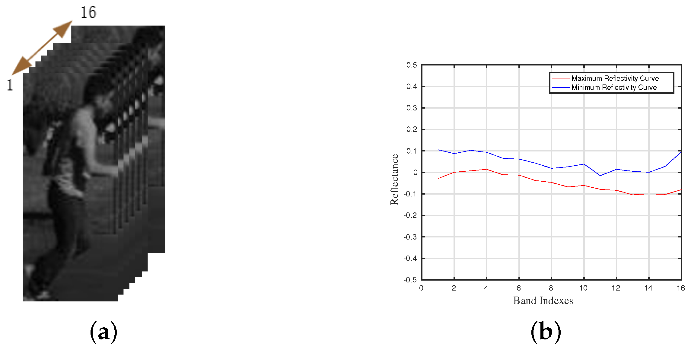
Remotesensing 15 01579 g001
Figure 2. The pretreatment of the proposed dimensionality reduction method. (a) The given ground truth of the first frame. (b) The extracted maximum spectral curve and minimum spectral curve from the local region in the ground truth.
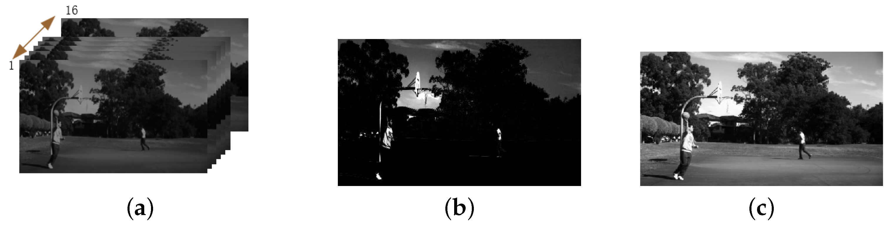
Remotesensing 15 01579 g002
Figure 3. The result of the proposed dimensionality reduction method. (a) The original hyperspectral image in the dataset. (b) The dimensionality reduction result of (a) using DRSD. (c) The dimensionality reduction result of (a) using PCA.
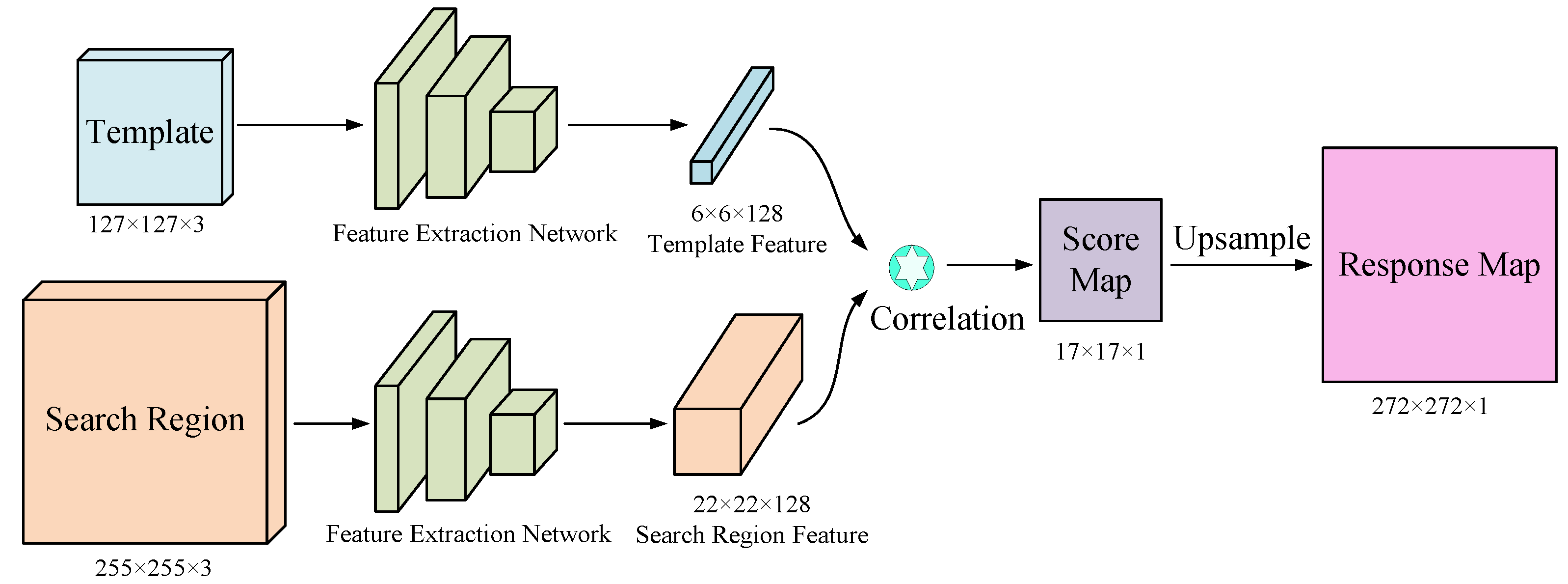
Remotesensing 15 01579 g003
Figure 4. The overall framework of SiamFC.
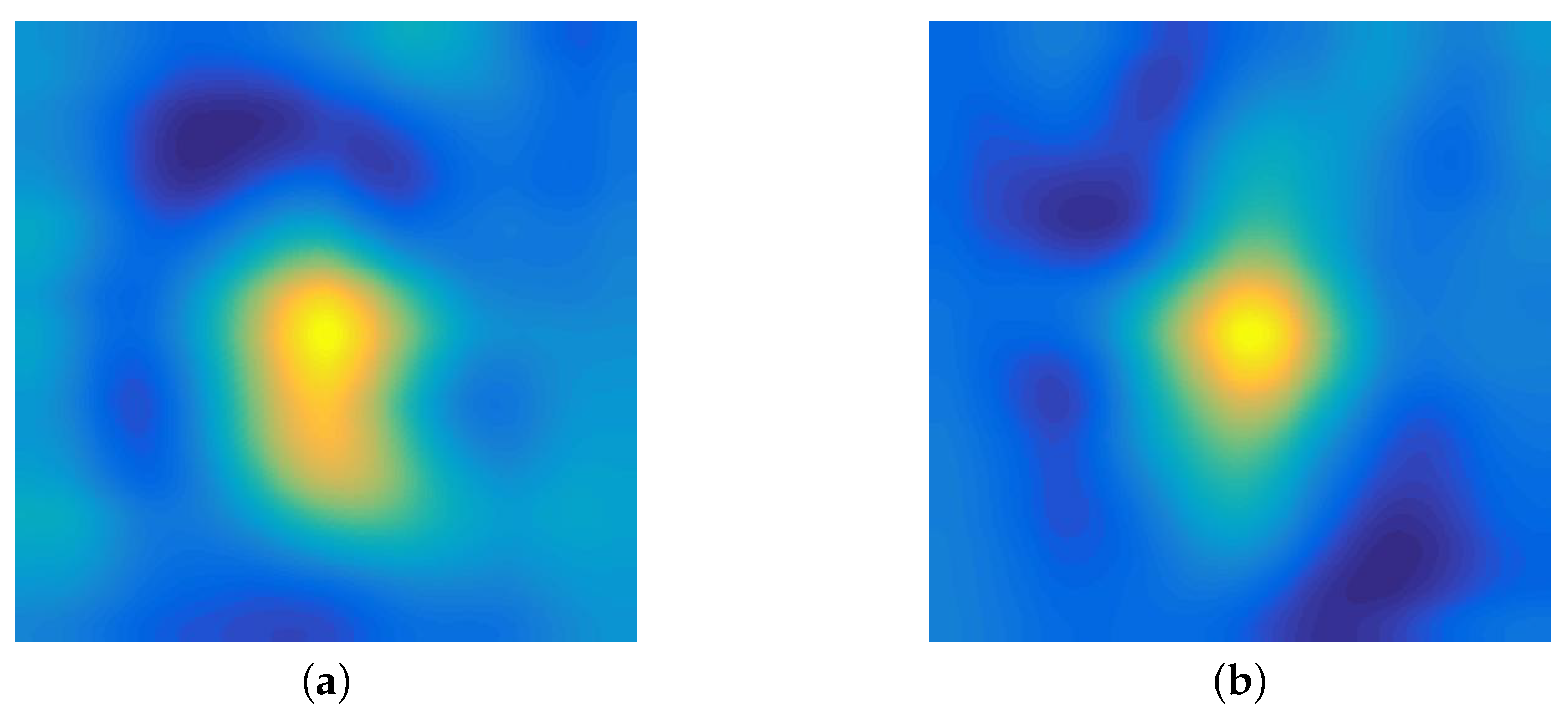
Remotesensing 15 01579 g004
Figure 5. A group of the initial response map and the adjacent response map in the experiments. (a) The initial response map. (b) The adjacent response map.
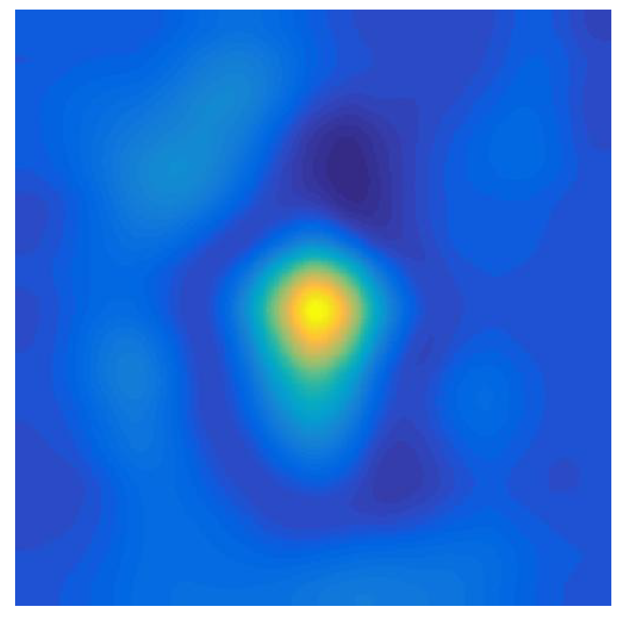
Remotesensing 15 01579 g005
Figure 6. The fused response map.
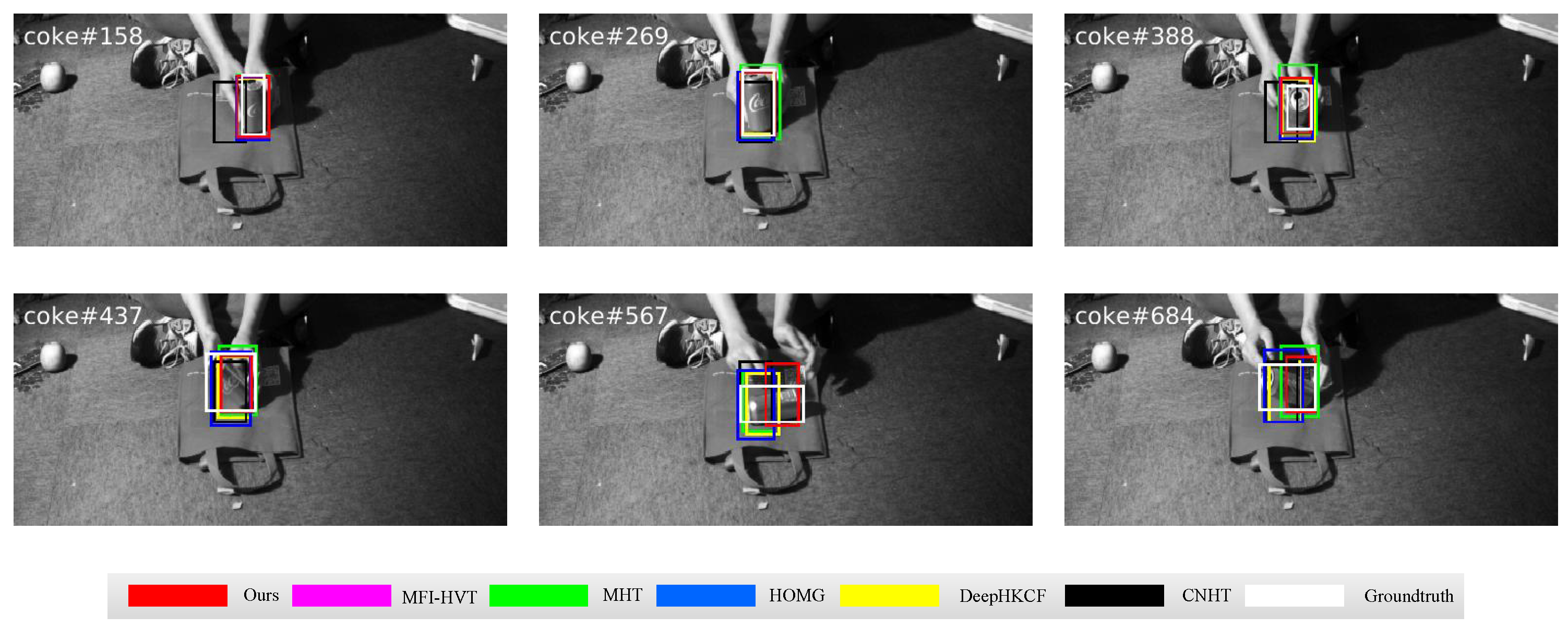
Remotesensing 15 01579 g006
Figure 7. Qualitative results on the coke sequence in comparative experiments.
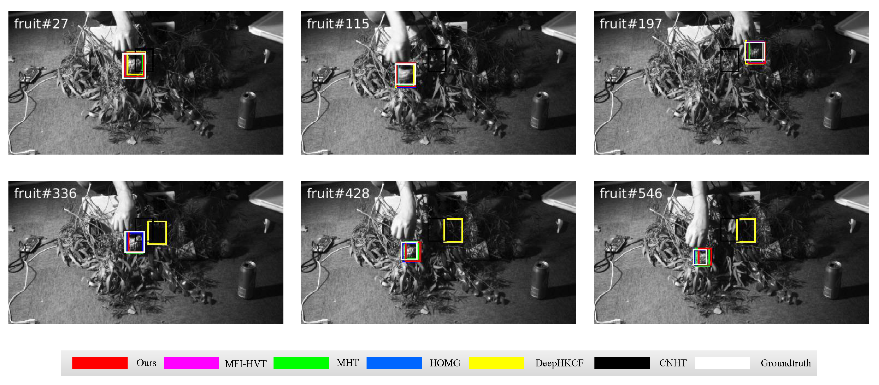
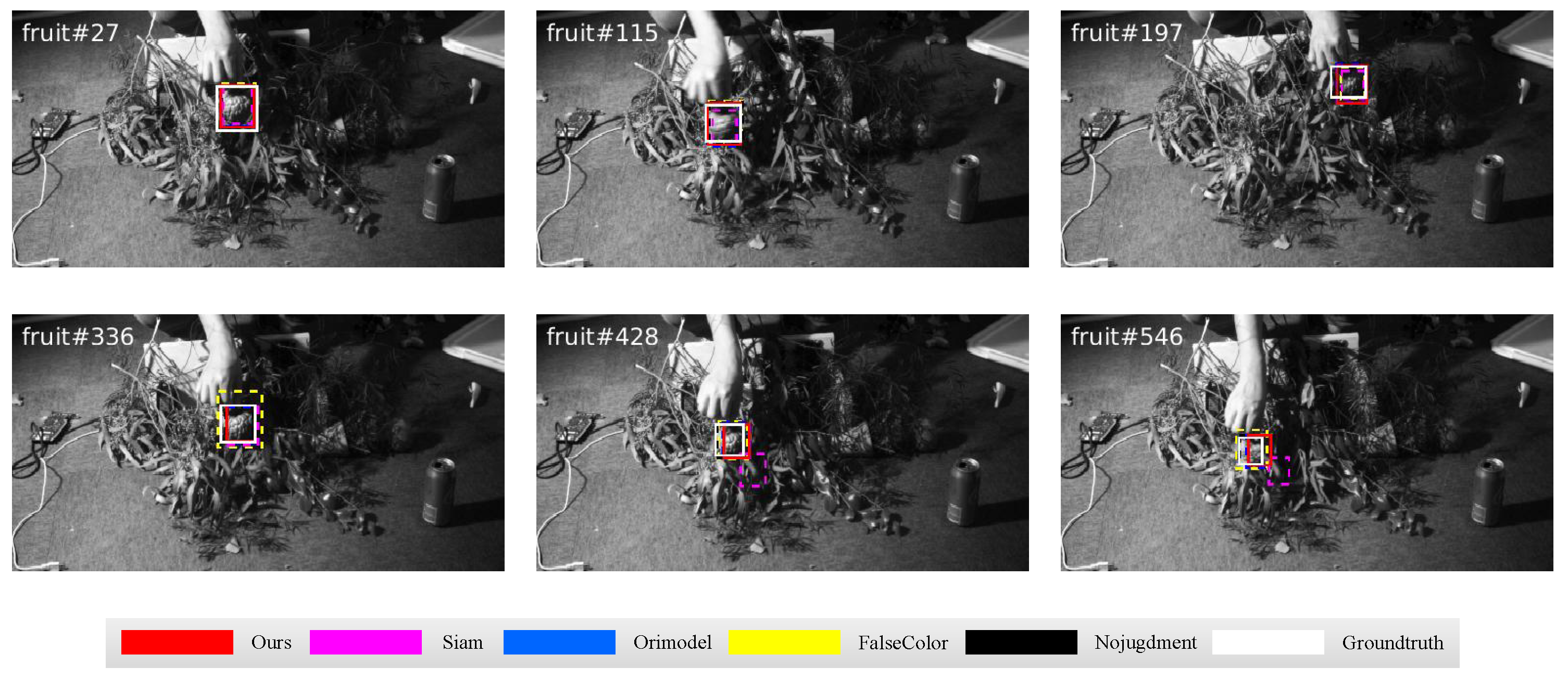
Remotesensing 15 01579 g007
Figure 8. Qualitative results on the fruit sequence in comparative experiments.
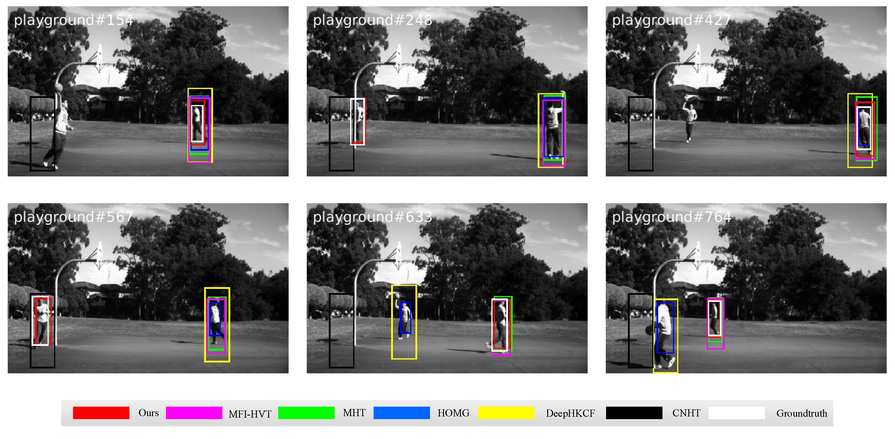
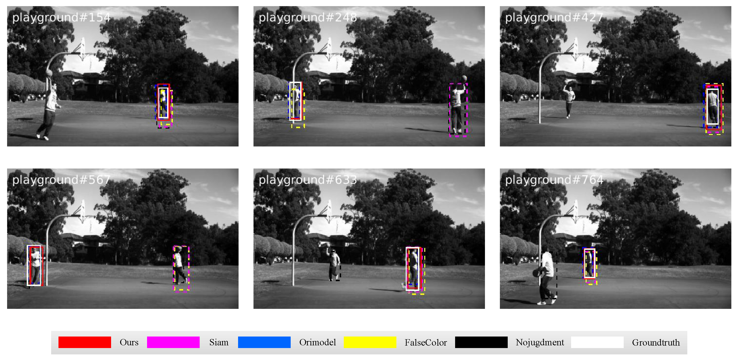
Remotesensing 15 01579 g008
Figure 9. Qualitative results on the playground sequence in comparative experiments.
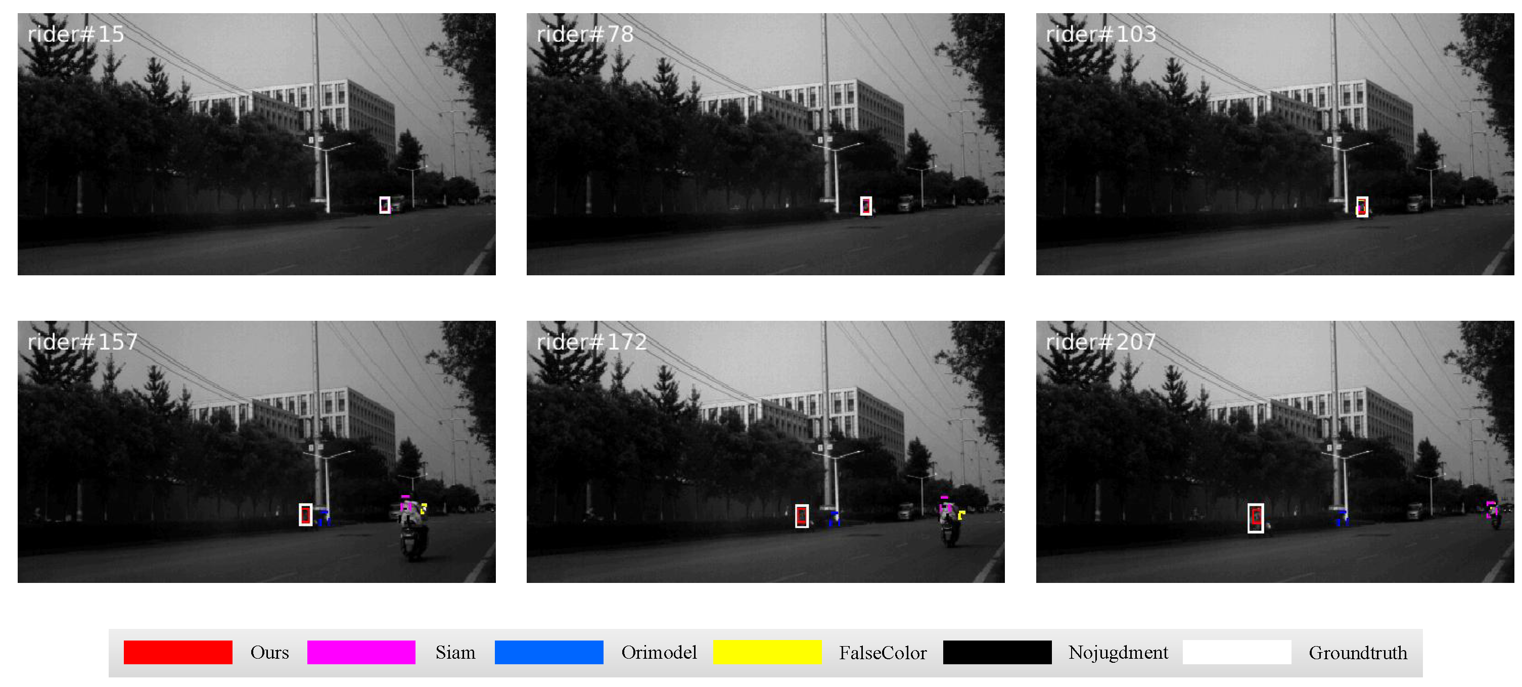
Remotesensing 15 01579 g009
Figure 10. Qualitative results on the rider sequence in comparative experiments.
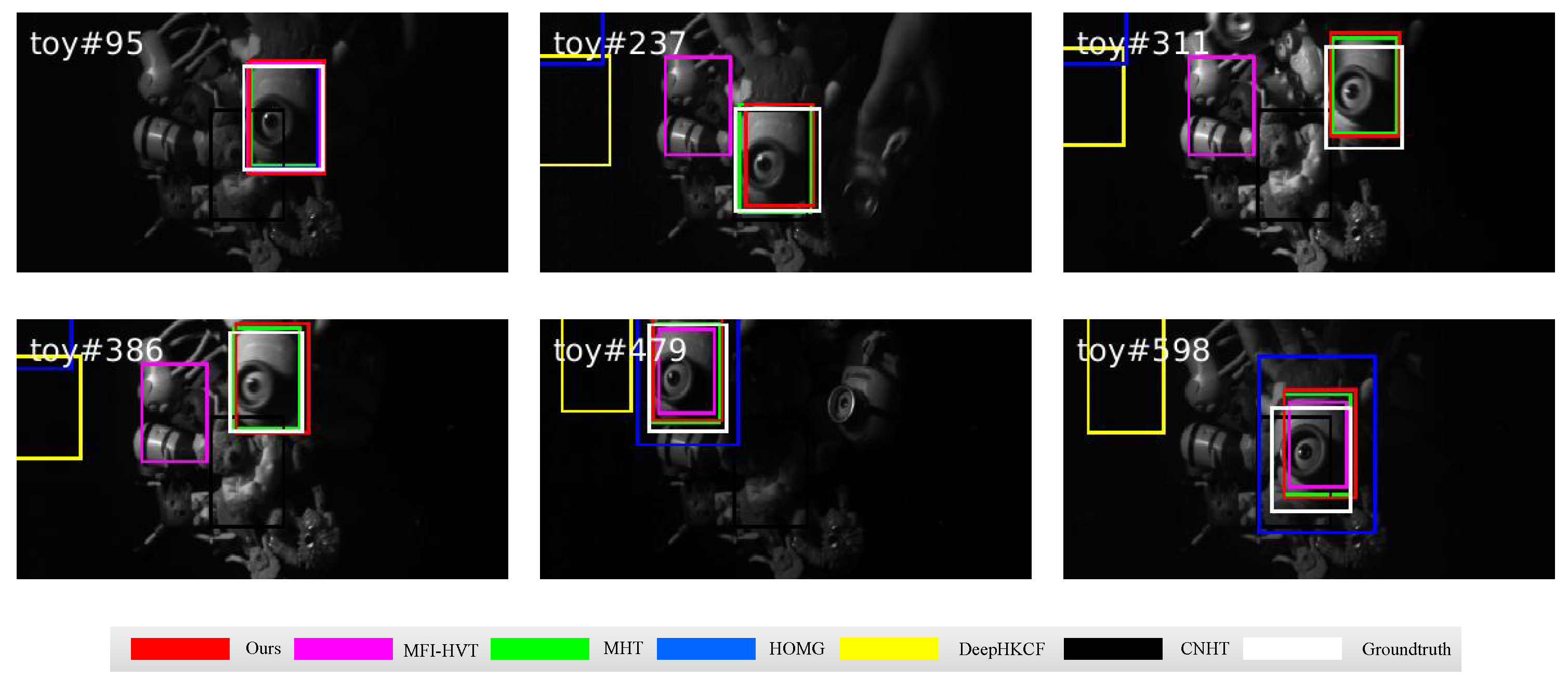
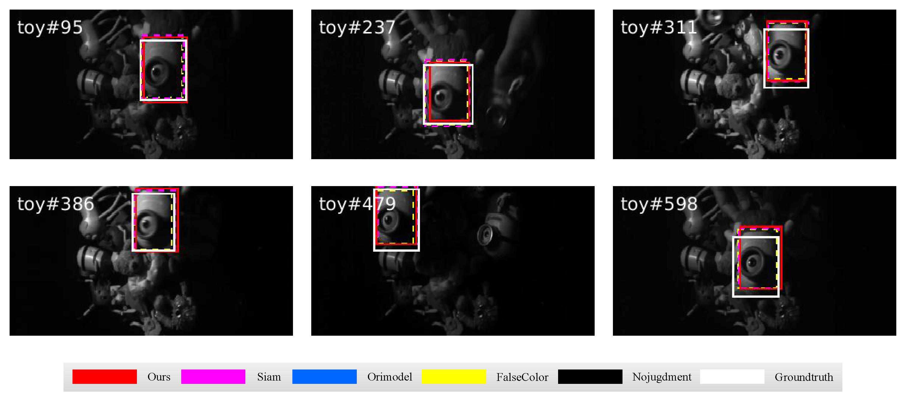
Remotesensing 15 01579 g010
Figure 11. Qualitative results on the toy sequence in comparative experiments.
Remotesensing 15 01579 g011
Figure 12. Quantitative results for all sequences in comparative experiments.
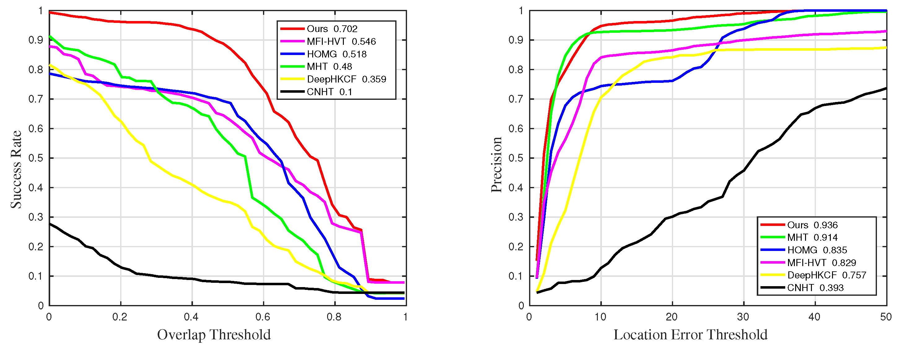
Remotesensing 15 01579 g012
Figure 13. Quantitative results for sequences with challenge BC in comparative experiments.
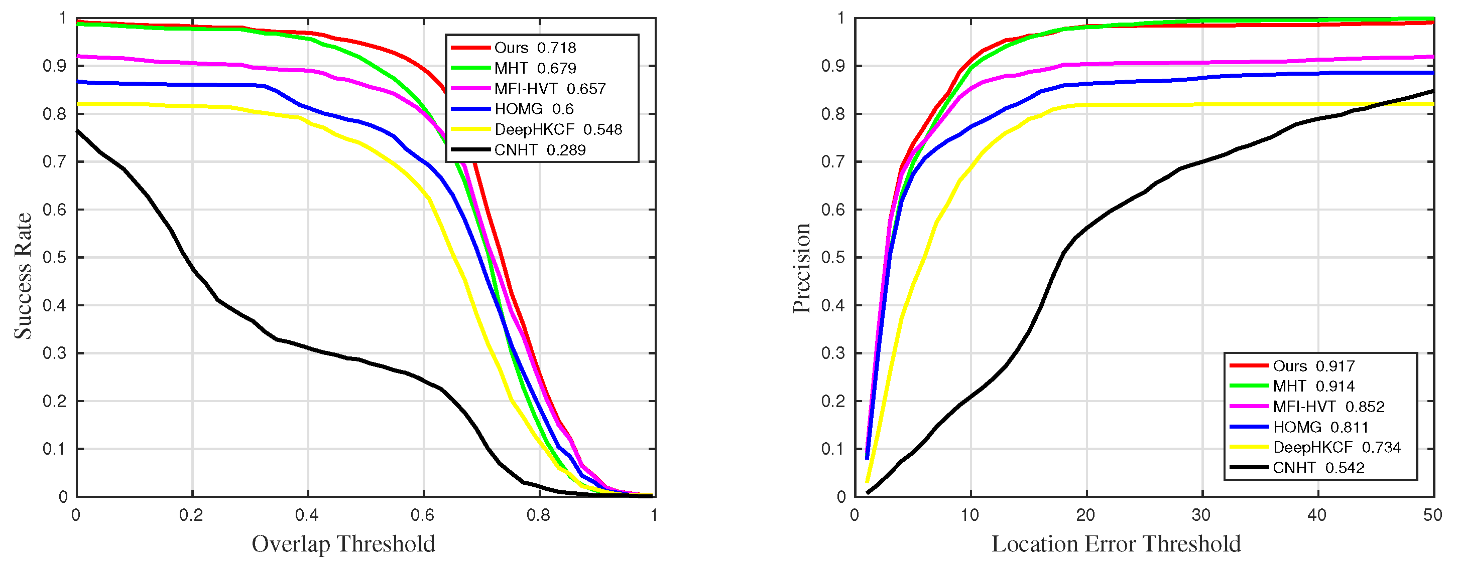
Remotesensing 15 01579 g013
Figure 14. Quantitative results for sequences with challenge IV in comparative experiments.
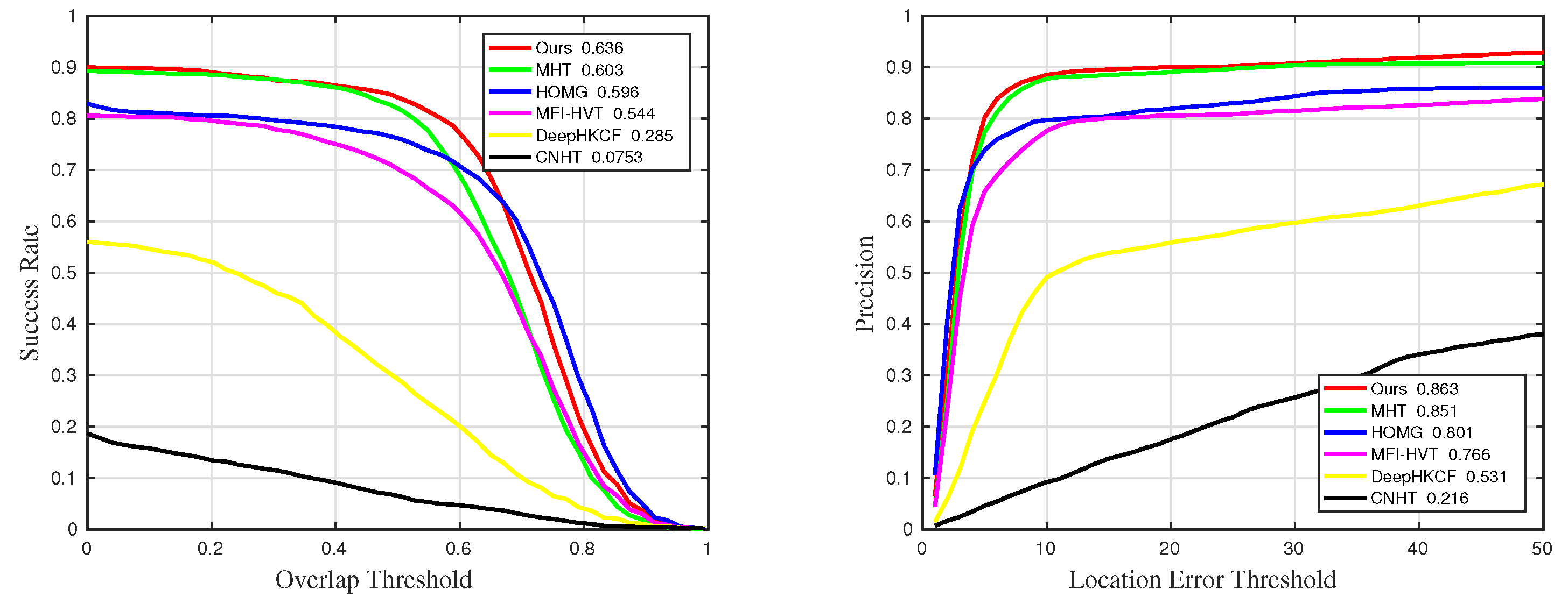
Remotesensing 15 01579 g014
Figure 15. Quantitative results for sequences with challenge OCC in comparative experiments.
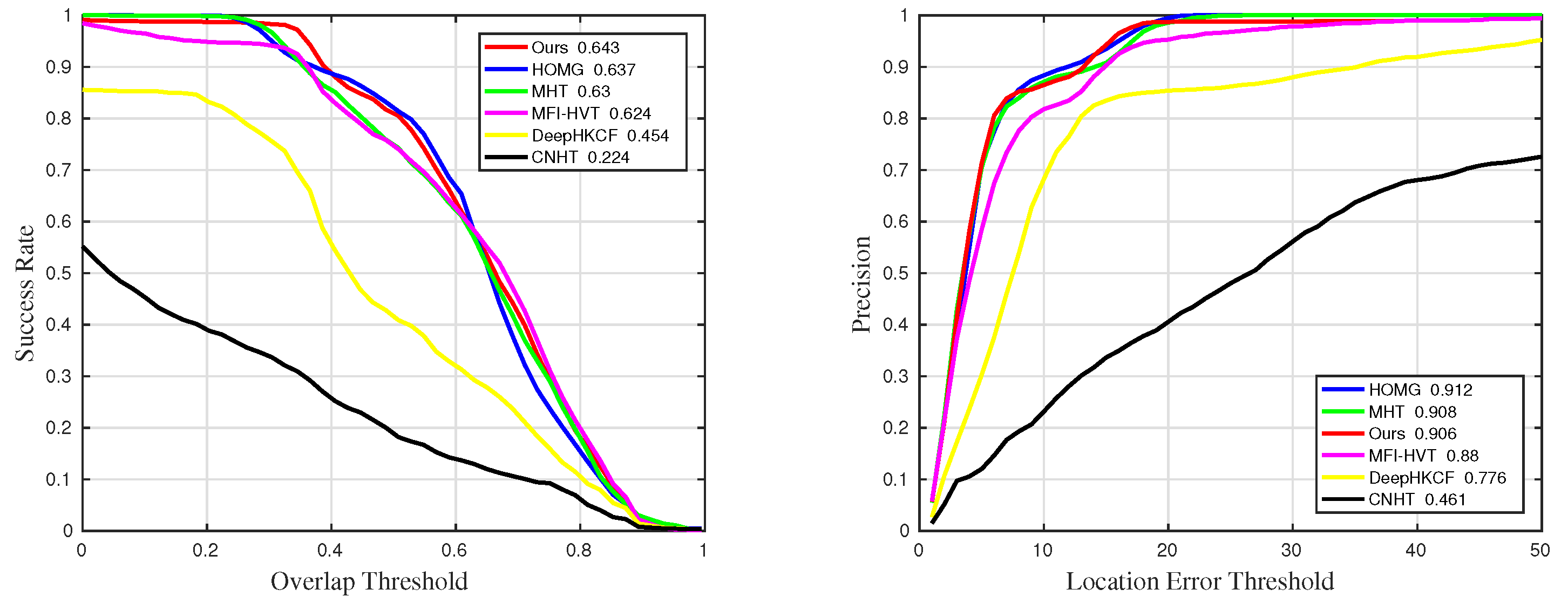
Remotesensing 15 01579 g015
Figure 16. Quantitative results for sequences with challenge RO in comparative experiments.
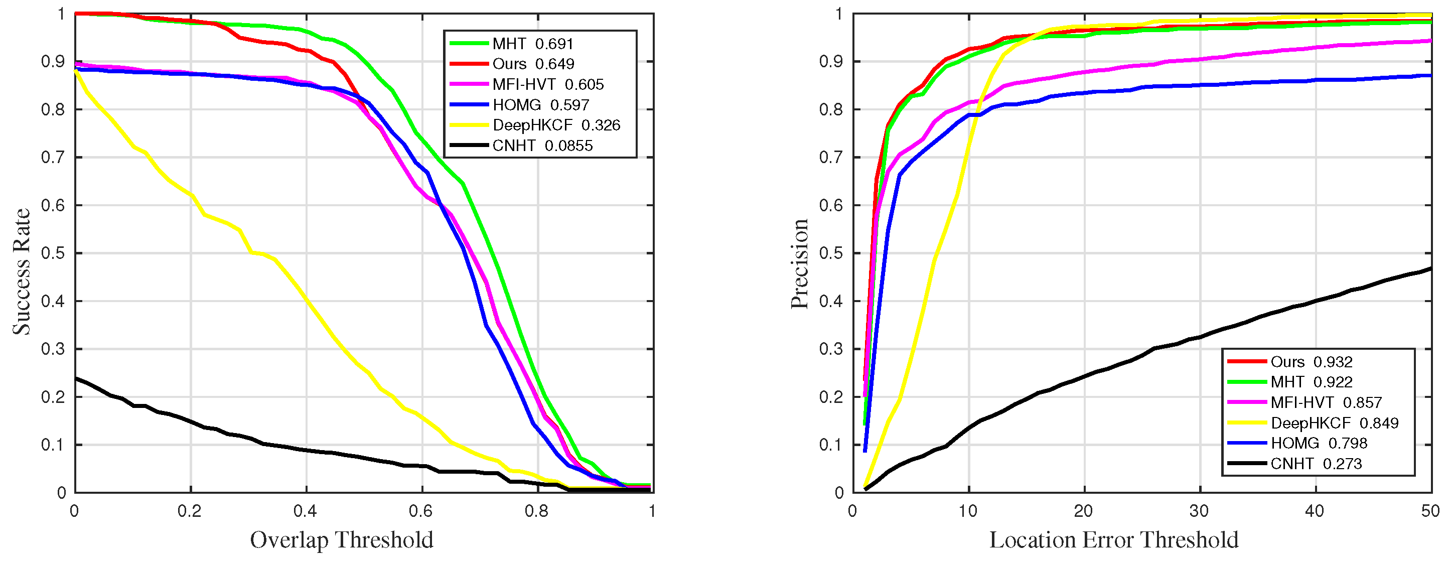
Remotesensing 15 01579 g016
Figure 17. Quantitative results for sequences with challenge SV in comparative experiments.
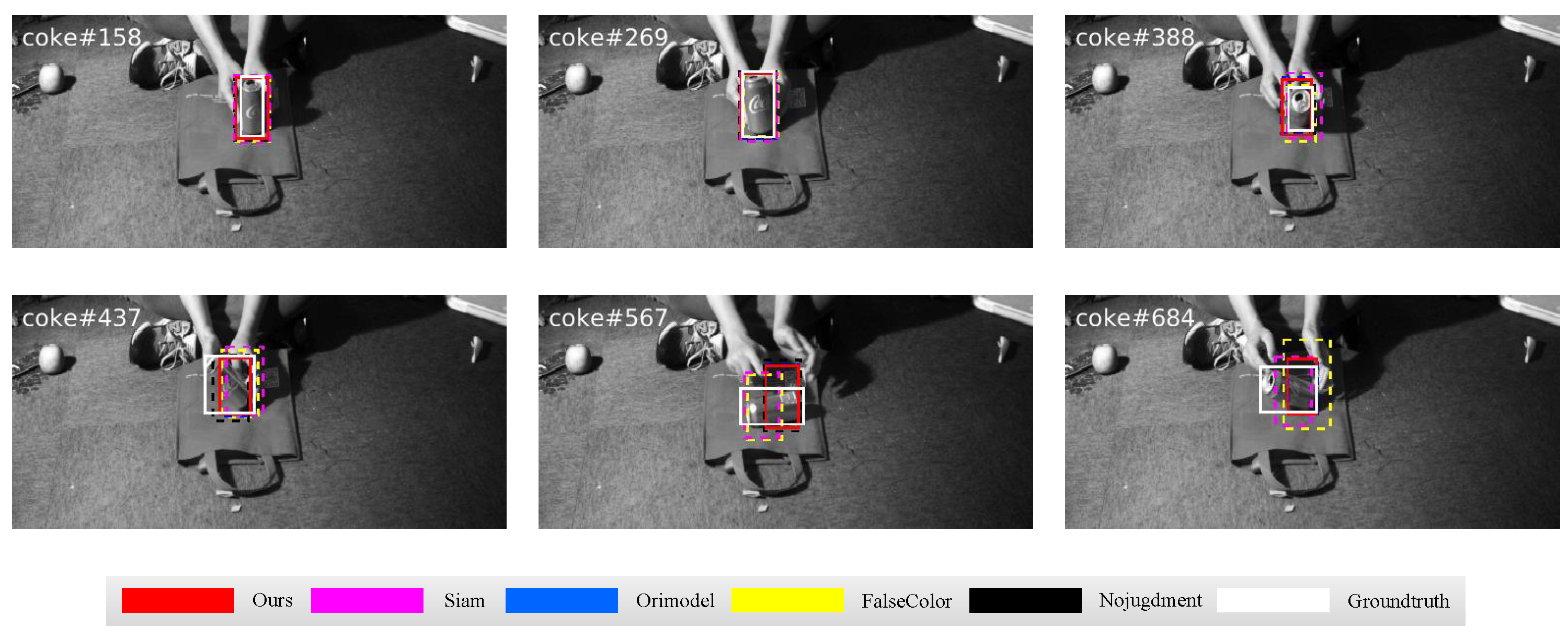
Remotesensing 15 01579 g017
Figure 18. Qualitative results on the coke sequence in ablation experiments.
Remotesensing 15 01579 g018
Figure 19. Qualitative results on the fruit sequence in ablation experiments.
Remotesensing 15 01579 g019
Figure 20. Qualitative results on the playground sequence in ablation experiments.
Remotesensing 15 01579 g020
Figure 21. Qualitative results on the rider sequence in ablation experiments.
Remotesensing 15 01579 g021
Figure 22. Qualitative results on the toy sequence in ablation experiments.
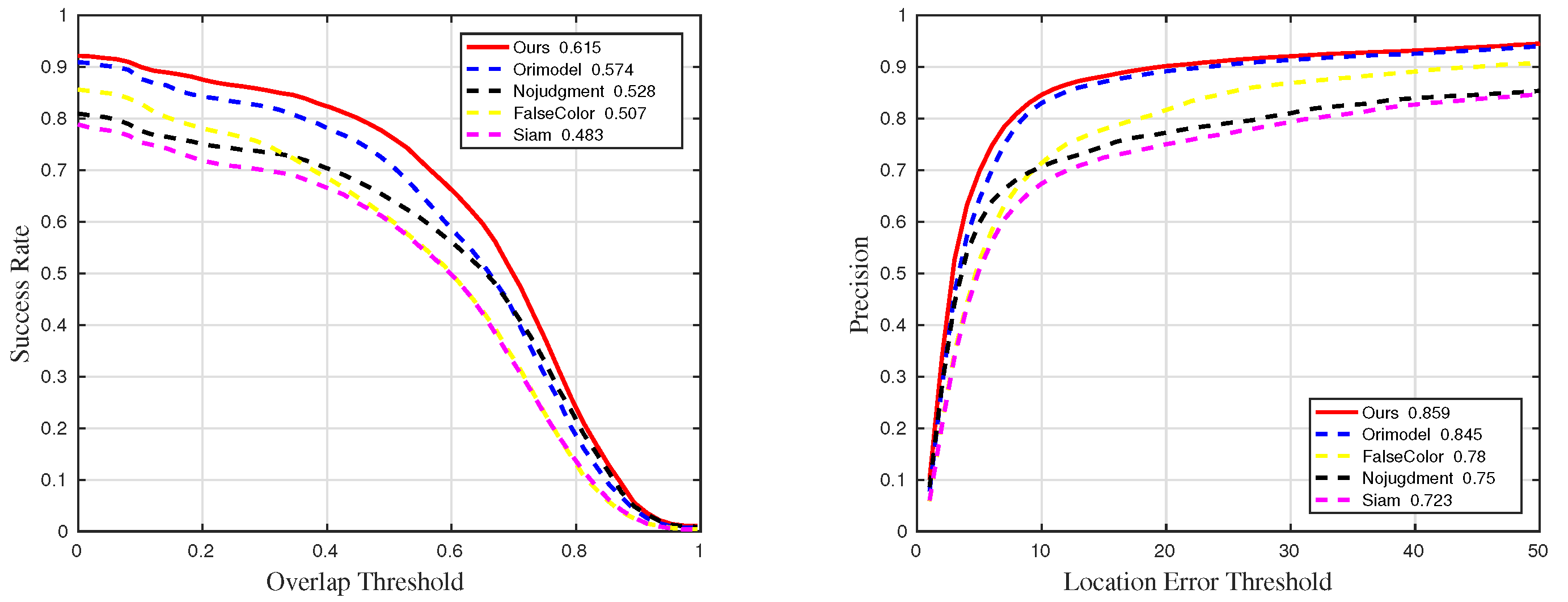
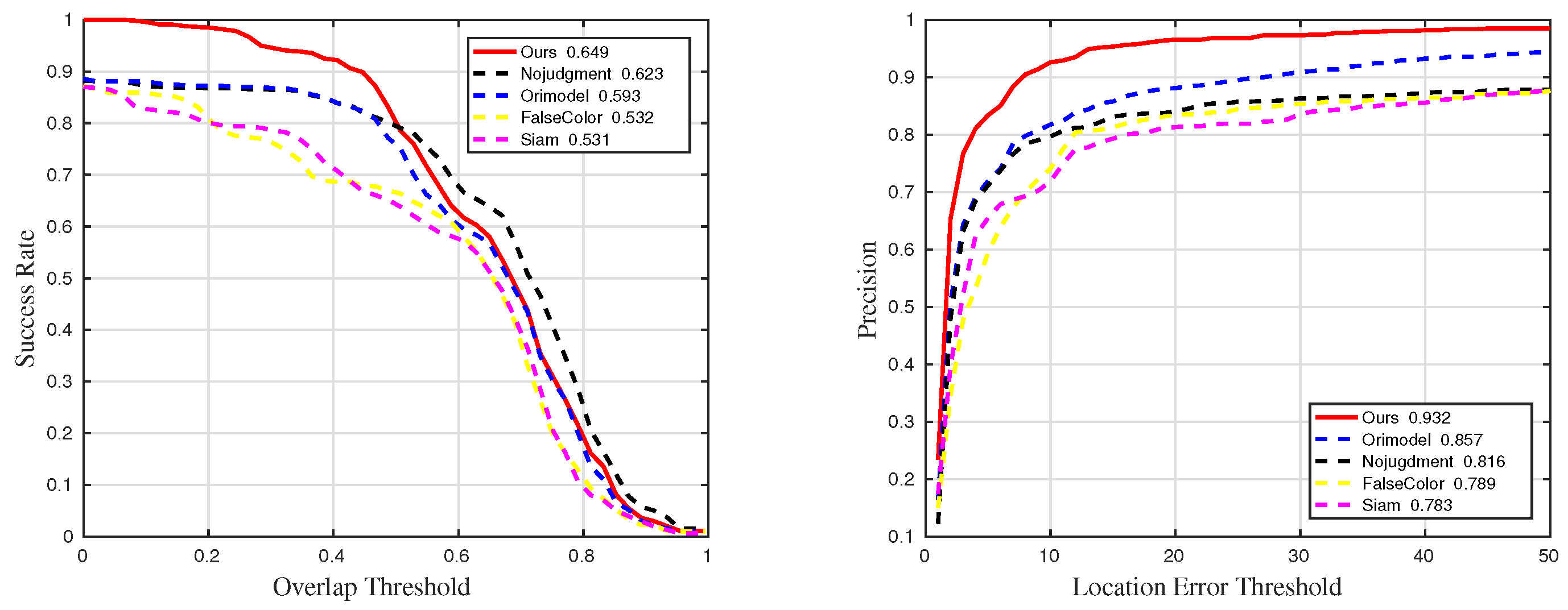
Remotesensing 15 01579 g022
Figure 23. Quantitative results for all sequences in ablation experiments.
Remotesensing 15 01579 g023
Figure 24. Quantitative results for sequences with challenge BC in ablation experiments.
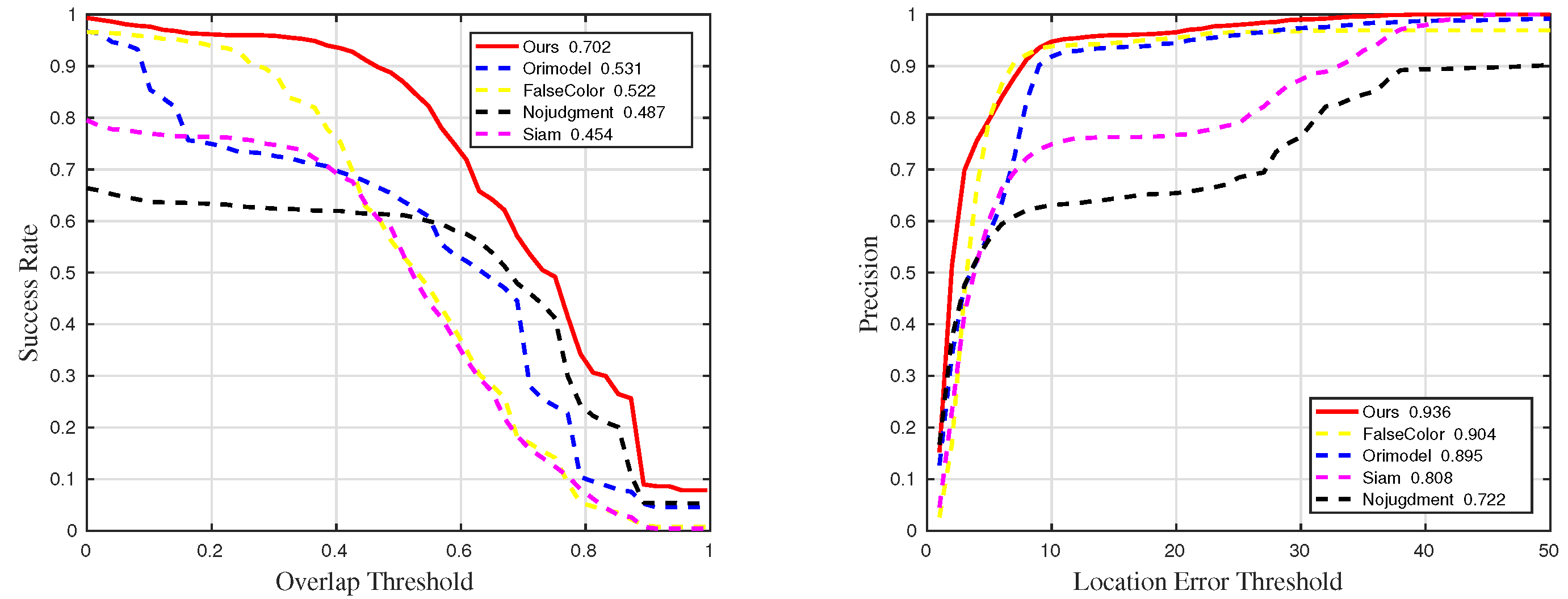
Remotesensing 15 01579 g024
Figure 25. Quantitative results for sequences with challenge IV in ablation experiments.
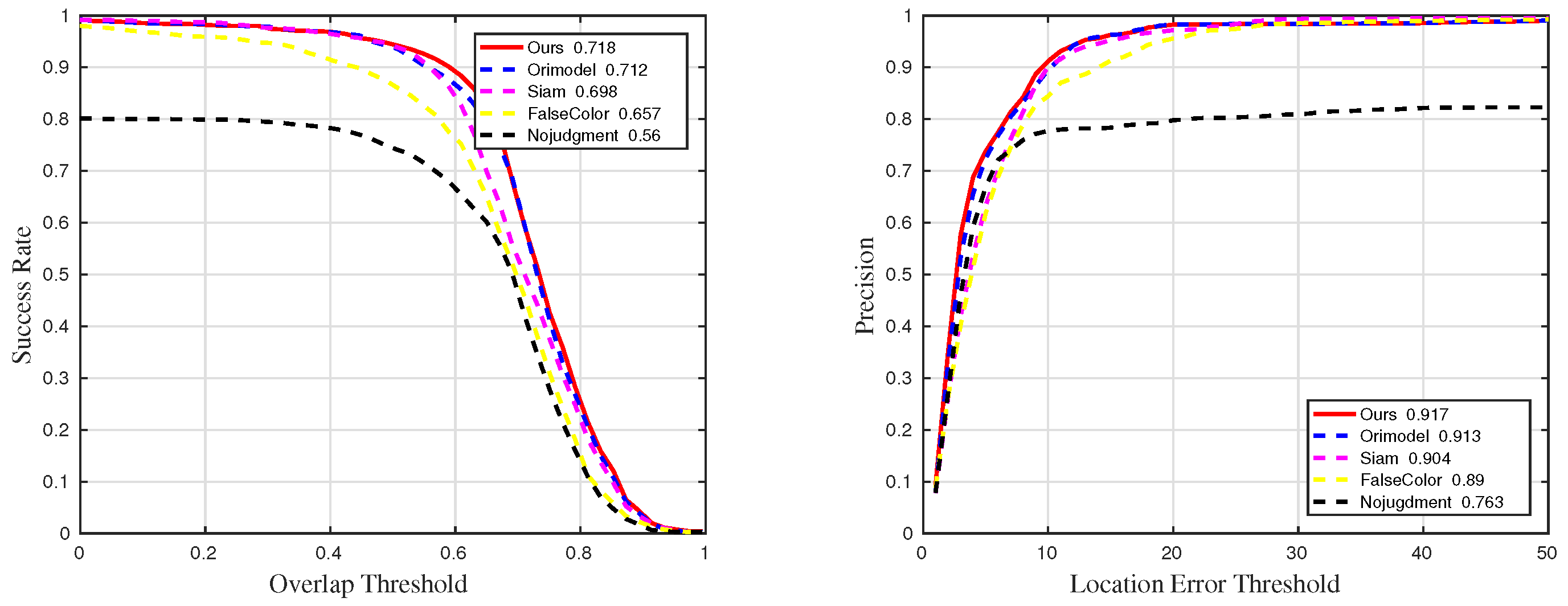
Remotesensing 15 01579 g025
Figure 26. Quantitative results for sequences with challenge OCC in ablation experiments.
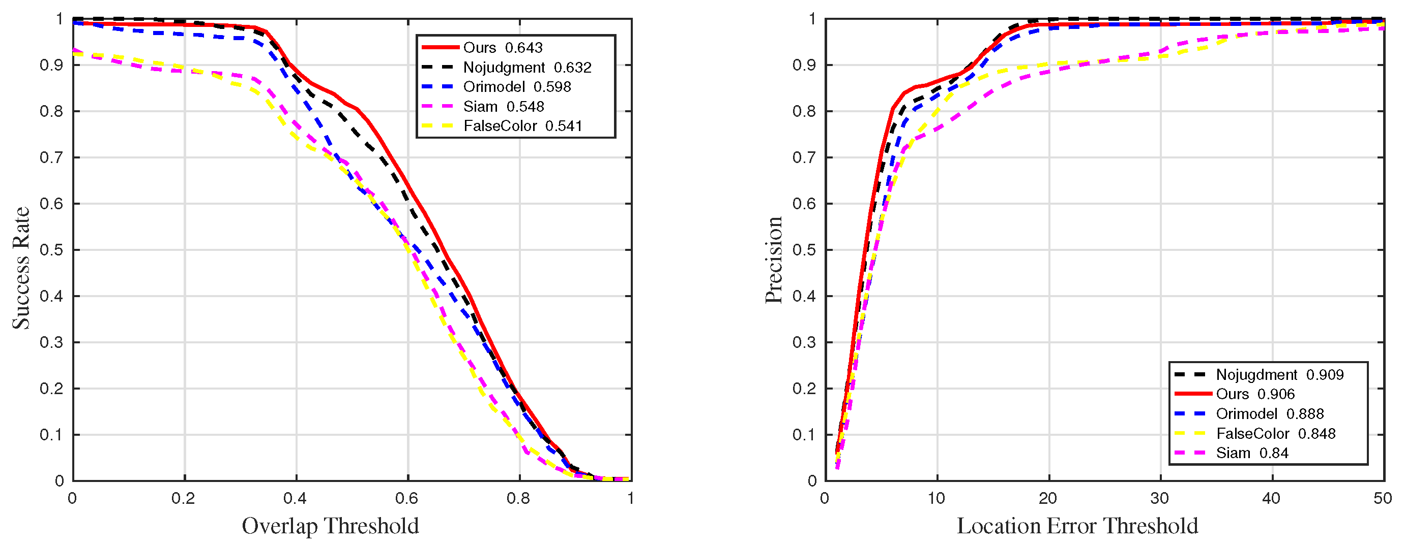
Remotesensing 15 01579 g026
Figure 27. Quantitative results for sequences with challenge RO in ablation experiments.
Remotesensing 15 01579 g027
Figure 28. Quantitative results for sequences with challenge SV in ablation experiments.
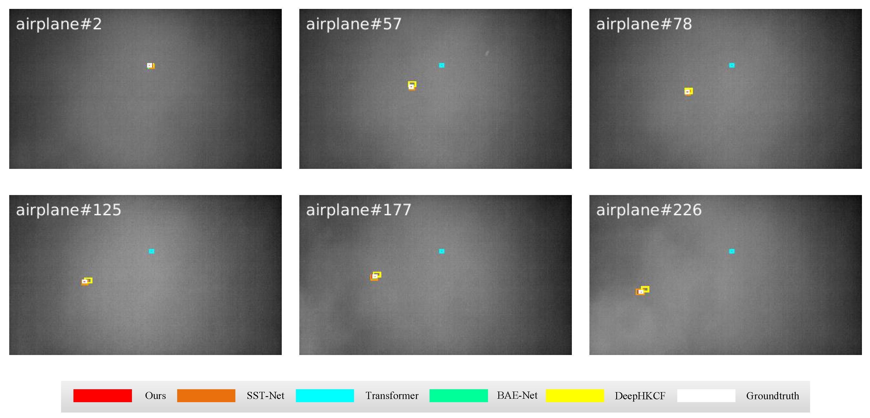
Remotesensing 15 01579 g028
Figure 29. Qualitative results of the airplane sequence in universality experiments.
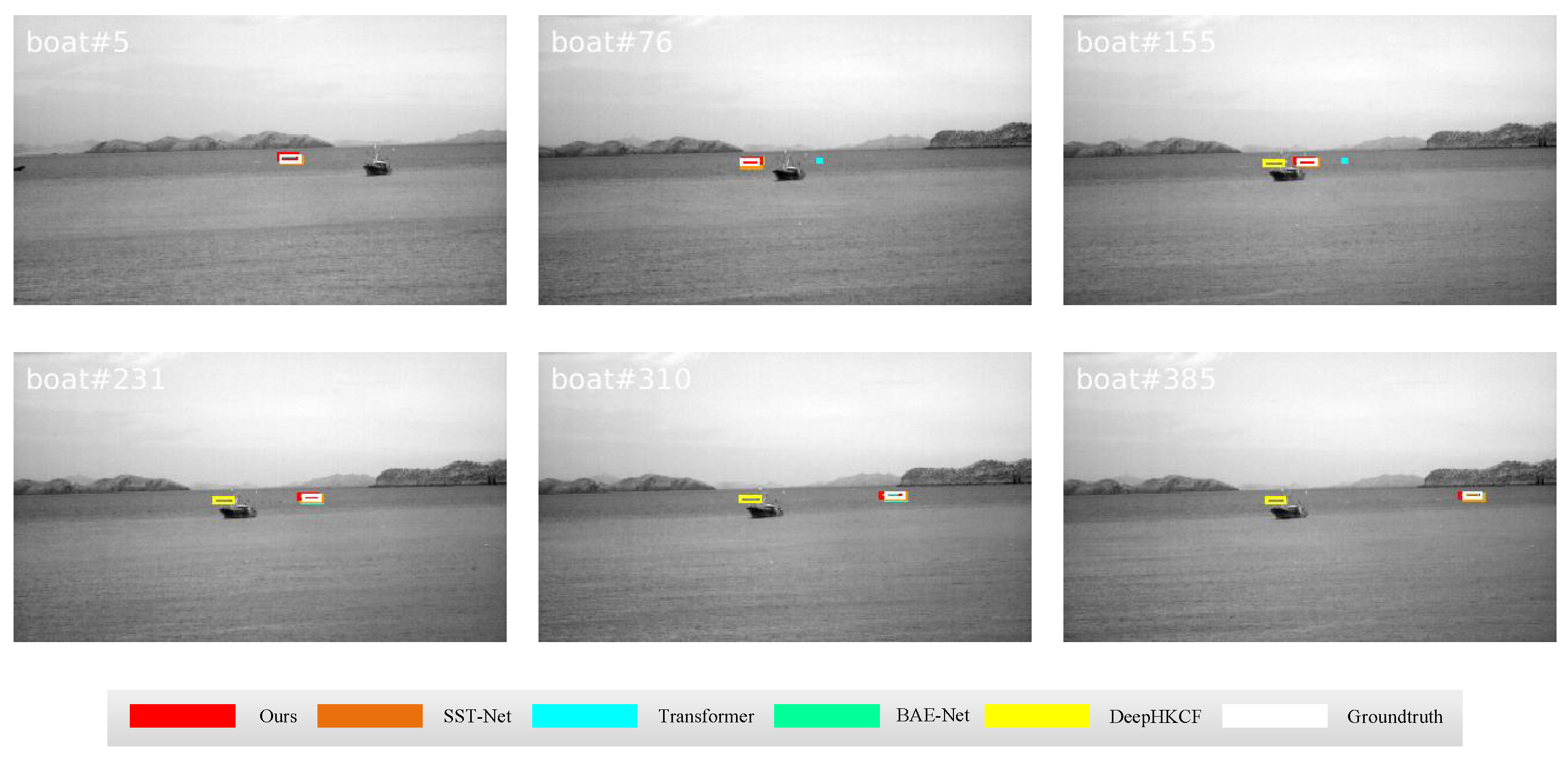
Remotesensing 15 01579 g029
Figure 30. Qualitative results on the boat sequence in universality experiments.
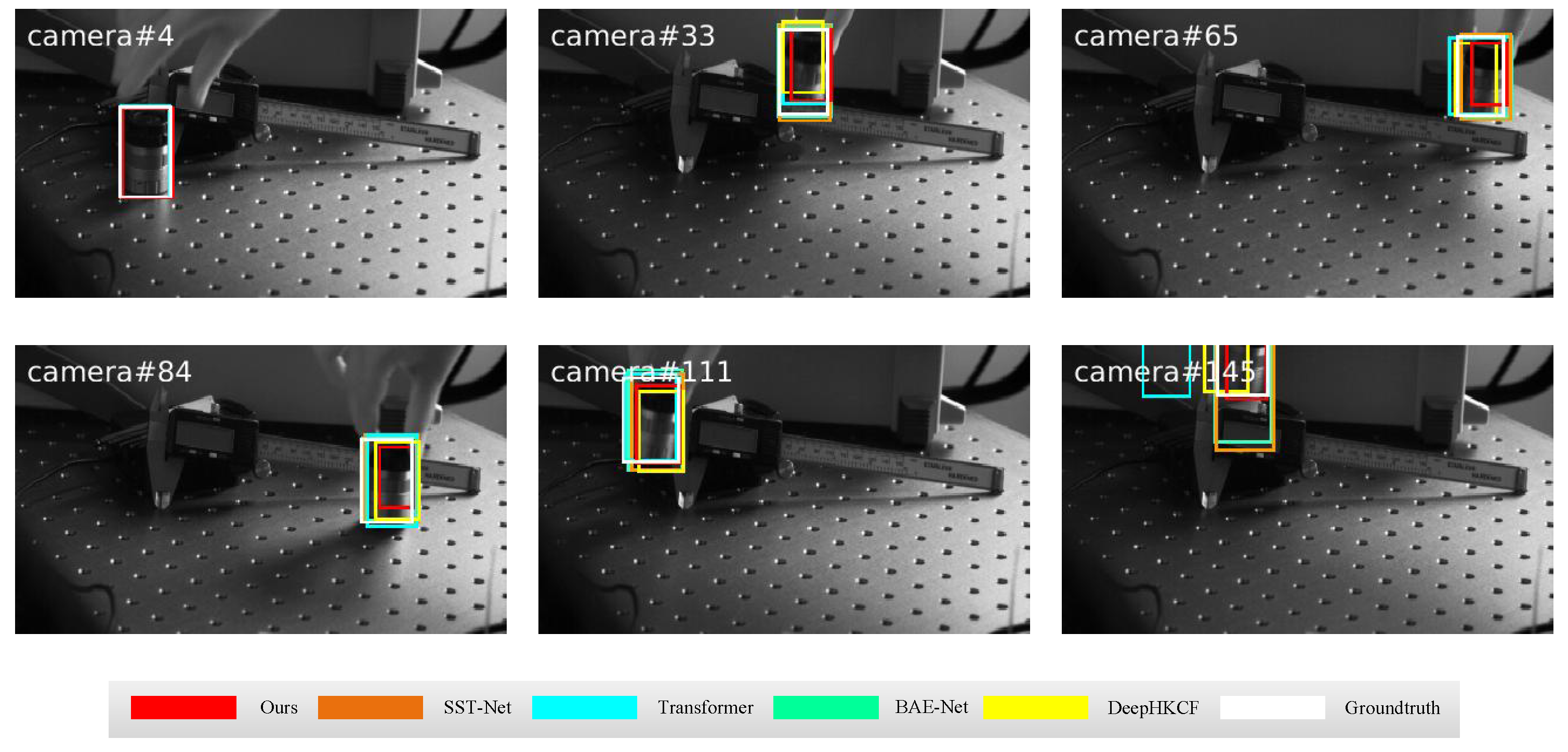
Remotesensing 15 01579 g030
Figure 31. Qualitative results on the camera sequence in universality experiments.
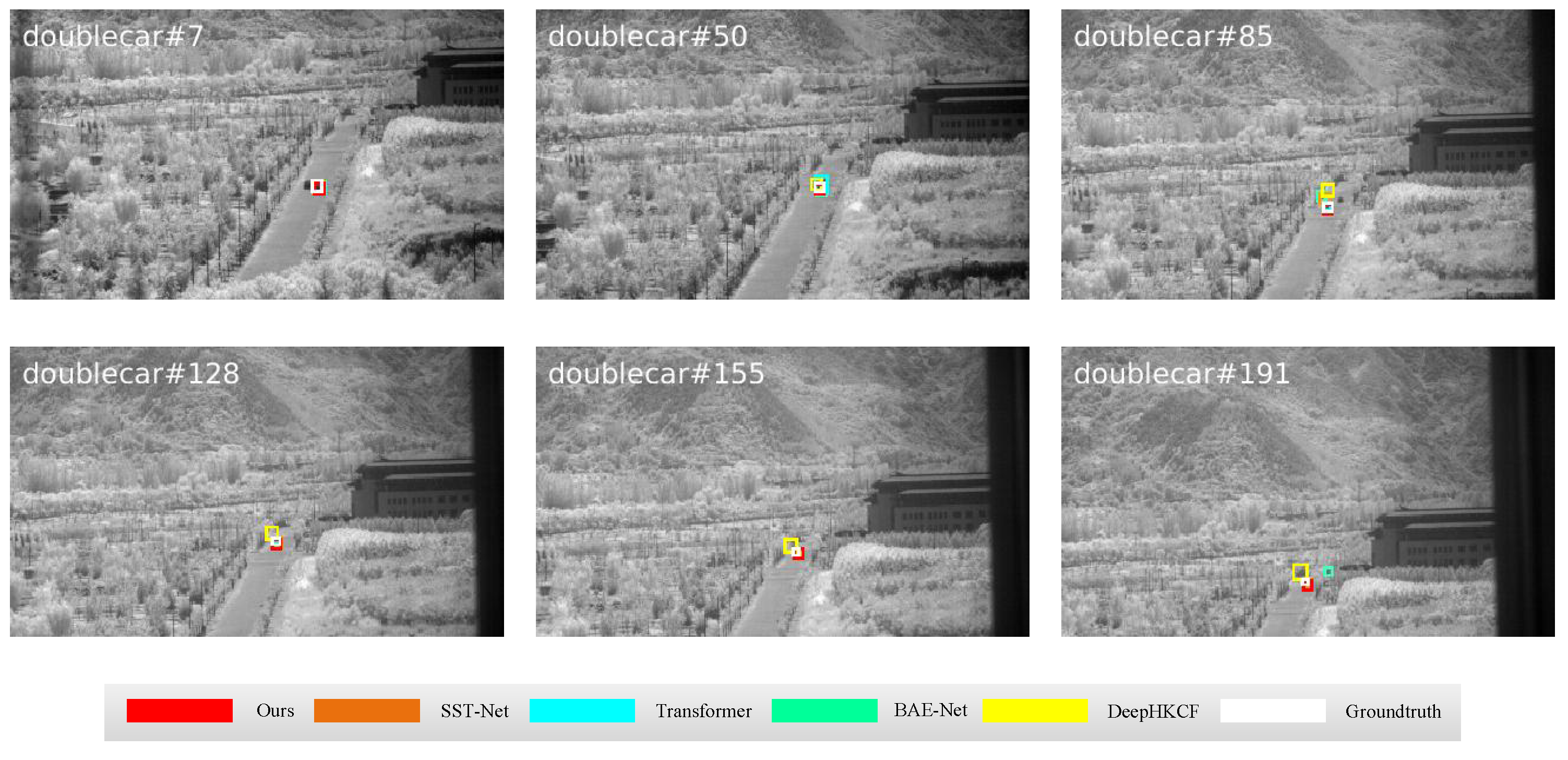
Remotesensing 15 01579 g031
Figure 32. Qualitative results on the doublecar sequence in universality experiments.
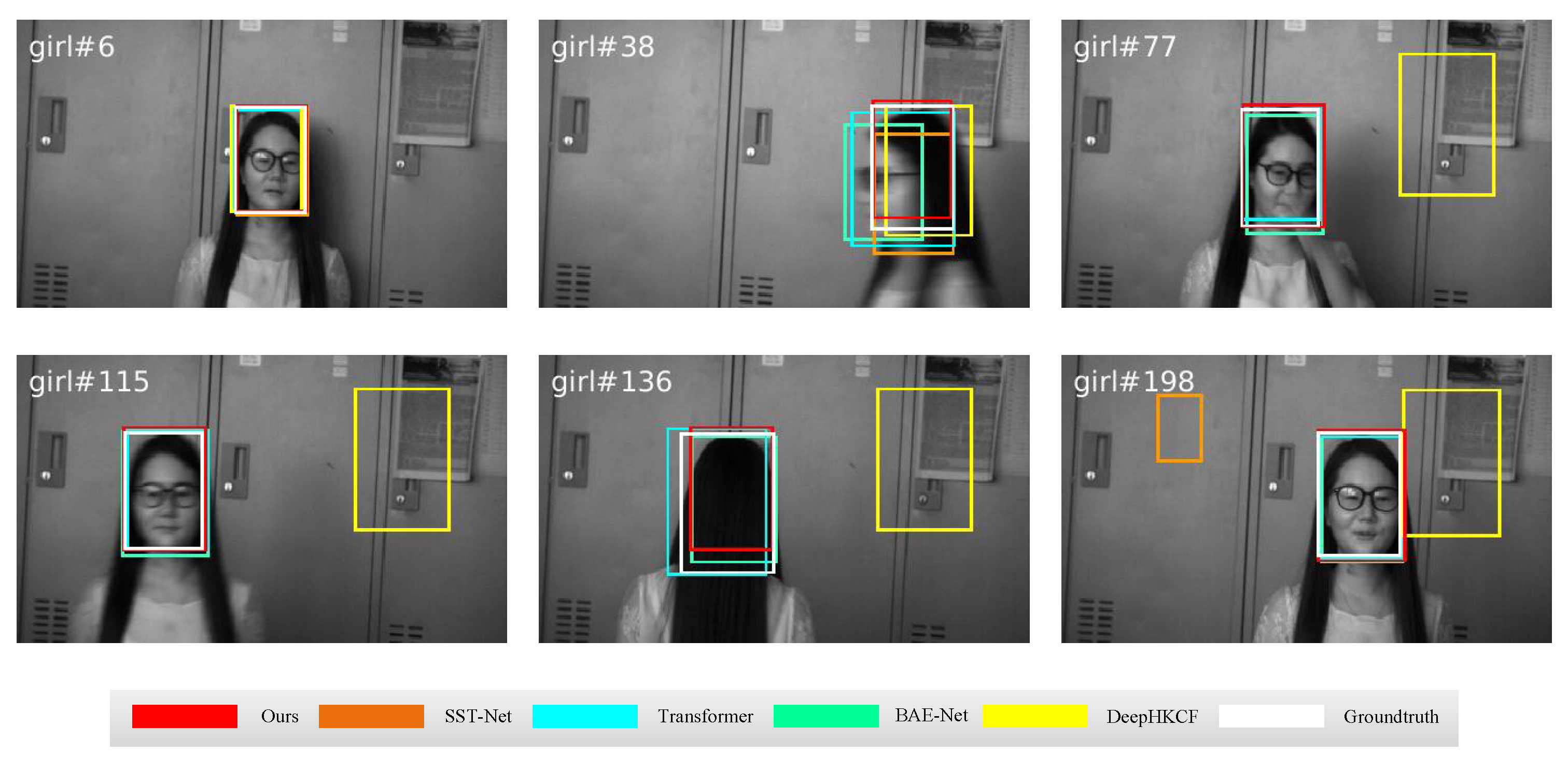
Remotesensing 15 01579 g032
Figure 33. Qualitative results on the girl sequence in universality experiments.
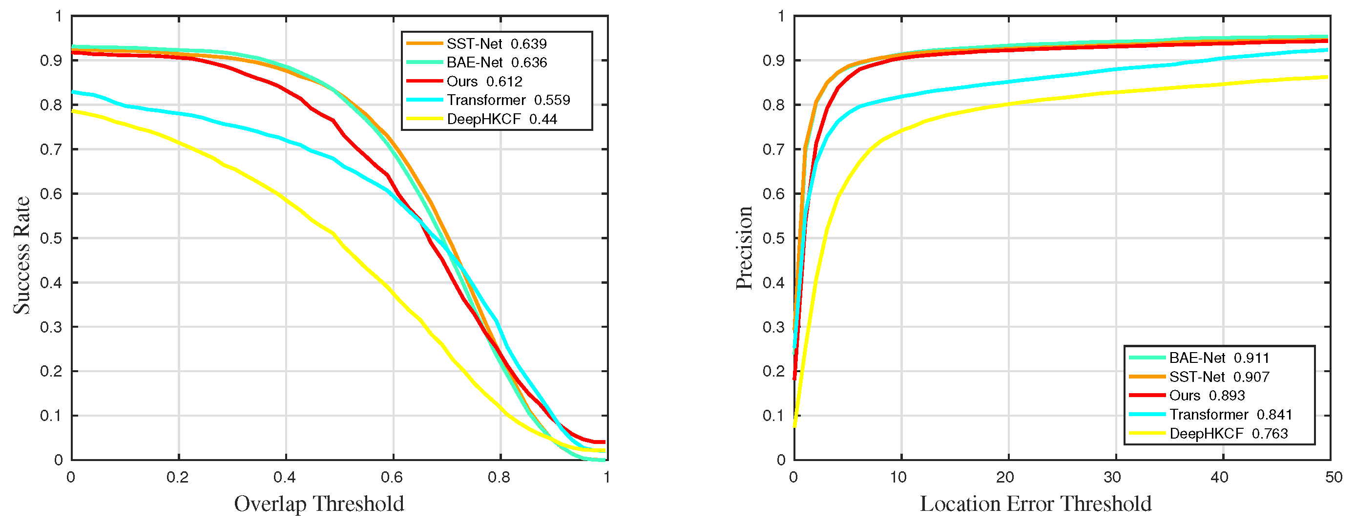
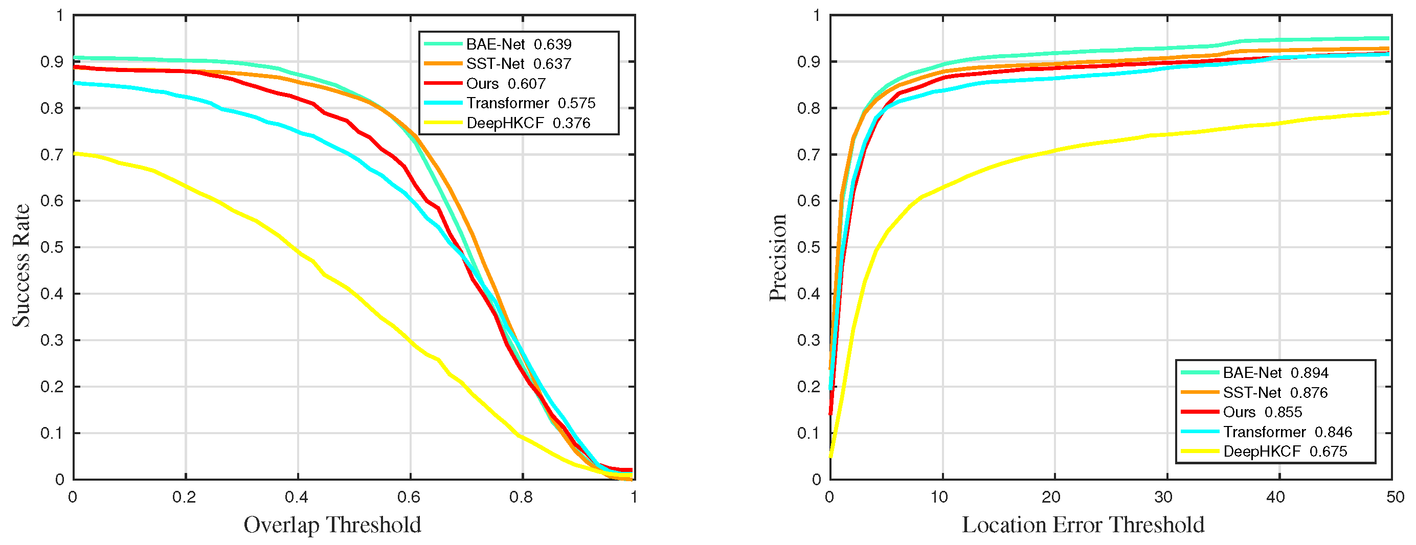
Remotesensing 15 01579 g033
Figure 34. Quantitative results for all sequences in universality experiments.
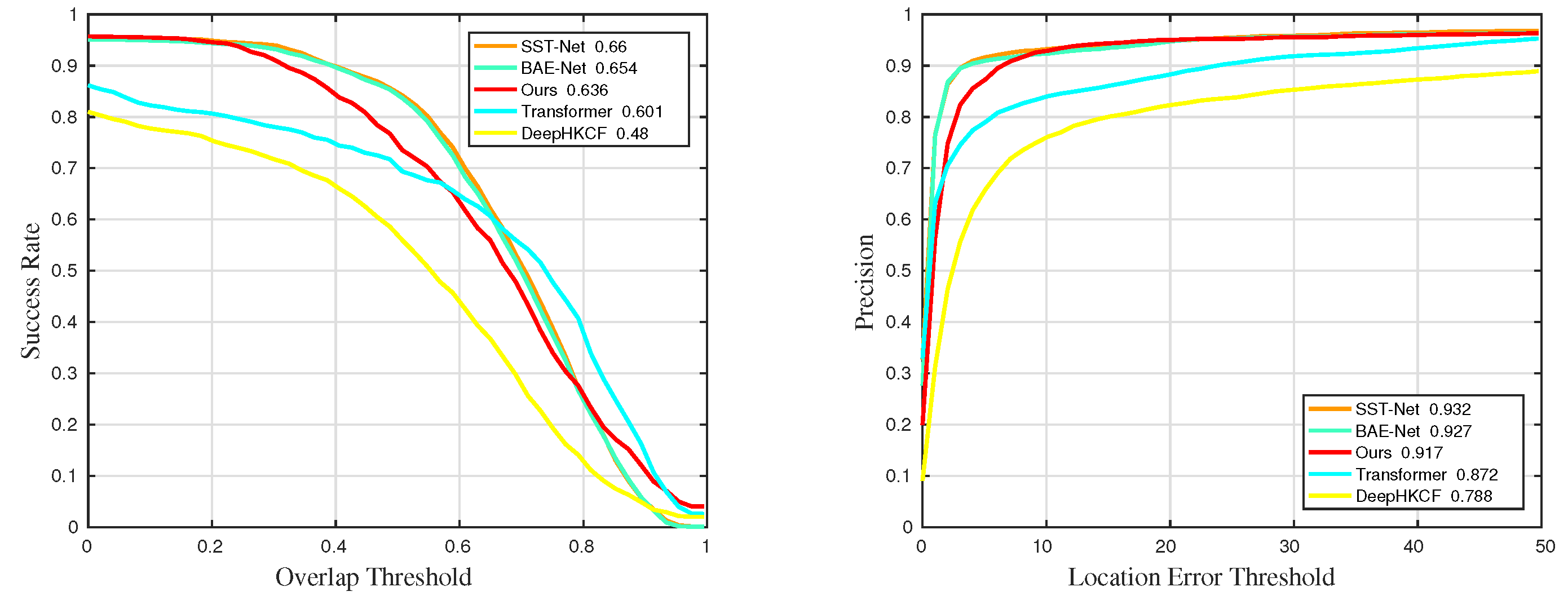
Remotesensing 15 01579 g034
Figure 35. Quantitative results for sequences with challenge BC in universality experiments.
Remotesensing 15 01579 g035
Figure 36. Quantitative results for sequences with challenge LR in universality experiments.
Remotesensing 15 01579 g036
Figure 37. Quantitative results for sequences with challenge OCC in universality experiments.
Remotesensing 15 01579 g037
Figure 38. Quantitative results for sequences with challenge RO in universality experiments.
Remotesensing 15 01579 g038
Figure 39. Quantitative results for sequences with challenge SV in universality experiments.
Remotesensing 15 01579 g039
Table 1. The details of success rate results in comparative experiments. The suffixes mean that the measurements are only counted in the sequences with the corresponding challenges. The best and the second-best results are marked in red and blue, respectively.
MethodsSucSuc_BCSuc_IVSuc_OCCSuc_ROSuc_SV
Ours0.6150.7020.7180.6360.6430.649
MHT0.5840.480.6790.6030.630.691
MFI-HVT0.5790.5460.6570.5440.6240.605
DeepHKCF0.3860.3590.5480.2850.4540.326
HOMG0.5710.5180.60.5960.6370.597
CNHT0.1580.10.2890.07530.2240.0855
Table 2. The details of precision results in comparative experiments. The suffixes mean that the measurements are only counted in the sequences with the corresponding challenges. The best and the second-best results are marked in red and blue, respectively.
MethodsPrePre_BCPre_IVPre_OCCPre_ROPre_SV
Ours0.8590.9360.9170.8630.9060.932
MHT0.8450.9140.9140.8510.9080.922
MFI-HVT0.8240.8290.8520.7660.880.857
DeepHKCF0.6760.7570.7340.5310.7760.849
HOMG0.8090.8350.8110.8010.9120.798
CNHT0.3460.3930.5420.2160.4610.273
Table 3. The details of success rate results in ablation experiments. The suffixes mean that the measurements are only counted in the sequences with the corresponding challenges. The best and the second-best results are marked in red and blue, respectively.
MethodsSucSuc_BCSuc_IVSuc_OCCSuc_ROSuc_SV
Ours0.6150.7020.7180.6360.6430.649
Orimodel0.5740.5310.7120.6010.5980.593
Nojudgment0.5280.4870.560.4590.6320.623
FalseColor0.5070.5220.6570.5070.5410.532
Siam0.4830.4540.6980.4850.5480.531
Table 4. The details of precision results in ablation experiments. The suffixes mean that the measurements are only counted in the sequences with the corresponding challenges. The best and the second-best results are marked in red and blue, respectively.
MethodsPrePre_BCPre_IVPre_OCCPre_ROPre_SV
Ours0.8590.9360.9170.8630.9060.932
Orimodel0.8450.8950.9130.8520.8880.857
Nojudgment0.750.7220.7630.6950.9090.816
FalseColor0.780.9040.890.7980.8480.789
Siam0.7230.8080.9040.7230.840.783
Table 5. The details of success rate results in universality experiments. The suffixes mean that the measurements are only counted in the sequences with the corresponding challenges. The best and the second-best results are marked in red and blue, respectively.
MethodsSucSuc_BCSuc_LRSuc_OCCSuc_ROSuc_SV
Ours0.6120.6360.5930.6270.6210.607
BAE-Net0.6360.6540.6010.5990.6630.639
SST-Net0.6390.660.5770.6110.660.637
Transformer0.5590.6010.4690.4030.6540.575
DeepHKCF0.440.480.4180.4950.4140.376
Table 6. The details of precision results in universality experiments. The suffixes mean that the measurements are only counted in the sequences with the corresponding challenges. The best and the second-best results are marked in red and blue, respectively.
MethodsPrePre_BCPre_LRPre_OCCPre_ROPre_SV
Ours0.8930.9170.9120.9580.8970.855
BAE-Net0.9110.9270.9070.9160.9240.894
SST-Net0.9070.9320.8710.9180.9240.876
Transformer0.8410.8720.8040.7550.9110.846
DeepHKCF0.7630.7880.8120.8360.7050.675
Table 7. The computational speed of the algorithms using the IMEC16 dataset.
MethodsOursMHTMFI-HVTDeepHKCFHOMGCNHT
FPS1.81.2 (CPU)0.851.71.4 (CPU)1 (CPU)
Table 8. The computational speed of the algorithms using the IMEC25 dataset.
MethodsOursBAE-NetSST-NetTransformerDeepHKCF
FPS0.860.480.40.80.94
Disclaimer/Publisher’s Note: The statements, opinions and data contained in all publications are solely those of the individual author(s) and contributor(s) and not of MDPI and/or the editor(s). MDPI and/or the editor(s) disclaim responsibility for any injury to people or property resulting from any ideas, methods, instructions or products referred to in the content.

