Abstract
Transmission line detection is the basic task of using UAVs for transmission line inspection and other related tasks. However, the detection results based on traditional methods are vulnerable to noise, and the results may not meet the requirements. The deep learning method based on segmentation may cause a lack of vector information and cannot be applied to subsequent high-level tasks, such as distance estimation, location, and so on. In this paper, the characteristics of transmission lines in UAV images are summarized and utilized, and a lightweight powerline detection network is proposed. In addition, due to the reason that powerlines often run through the whole image and are sparse compared to the background, the FPN structure with Hough transform and the neck structure with multi-scale output are introduced. The former can make better use of edge information in a deep neural network as well as reduce the training time. The latter can reduce the error caused by the imbalance between positive and negative samples, make it easier to detect the lines running through the whole image, and finally improve the network performance. This paper also constructs a powerline detection dataset. While the net this paper proposes can achieve real-time detection, the f-score of the detection dataset reaches 85.6%. This method improves the effect of the powerline extraction task and lays the groundwork for subsequent possible high-level tasks.
1. Introduction
The unobstructed transmission lines and safe operation of various electrical equipment are the hardware foundation for the stability and reliability of the power grid system. In order to ensure the safe and stable operation of the power system, major power grid companies must arrange regular inspections of the power supply equipment. In recent years, researchers have been attracted by the excellent performance of small aircrafts, such as drones in low-altitude scenarios, and have made many advances in multiple fields including transmission line detection. Compared with human inspectors, drones can be more cost-effective in terms of time and space, more efficient, and more operationally flexible. Using their carried cameras, drones can obtain image data. In the acquired image data, the straight-line features of power lines often exhibit the following characteristics:
- (1)
- The transmission cable extends widely through the global image. The transmission wire can be roughly represented as a straight line over the entire image from a UAV flying at a low altitude and from the UAV’s perspective.
- (2)
- It can be approximated as a straight line. Due to the close proximity to the cable in the UAV image, the gravitational radian can be disregarded, allowing for a close approximation of a straight line.
Long-term research has been conducted on transmission line detection, and numerous researchers have developed a transmission line detection approach based on conventional image algorithms. Traditional methods [1] are often based on prior knowledge or gradient changes in the image itself, which are easy to misdetect. The line segment identification algorithm, which depends on the Hough transform [2], frequently requires that the edges of the image are extracted first because it is not resistant to changes in light. Furthermore, the texture information in the image is ignored. With the rise of deep learning, the rapid development of target detection methods based on deep learning, YOLO (you only look once) series [3,4,5], Fast-RCNN (Fast Region-based Convolutional Network) [6,7,8], and other algorithms have been particularly good in recent years, and these methods have achieved excellent performance in many fields of computer vision. In addition, many academics have suggested integrating the deep learning approach into straight-line detection in order to incorporate the literature and to use the straight line as a type of target to detect the straight line using the given detection method.
In this paper, a deep learning network for the detection of transmission lines was proposed, where the line segment is represented with the midpoint and two offset endpoints from the midpoint. The network utilizes the FPN (Feature pyramid Network) structure with the introduction of the Hough transform, which has the advantage of using points to represent lines in the Hough domain and thus introduces a parameterized description of the lines into the network. Additionally, because the transmission lines frequently cover the entire image, the network is output at various scales in this scenario to improve its effectiveness. Finally, the results are fused using the NMS (Non-Maximum Suppression) algorithm. The experimental findings demonstrate that the addition of the Hough FPN can speed up convergence and enhance the ability to discern straight lines. This paper also created a dataset for line target detection that may be used to identify line targets by tagging the current line segmentation dataset with images of transmission lines found on the network. Using the dataset we suggested, the model of this paper performed with a 0.86 f-score, 0.85 precision, and 0.88 recall.
2. Literature Review
2.1. Hough Transform
The Hough transform (HT) was first put forth in ref. [2] for the automated interpretation of images taken in bubble chambers. Duda and Hart [9] use the corner radius rather than the slope–intercept parameter, which makes the computation even simpler and avoids the scenario where the slope of the line tends to infinity. Illingworth and Kittler [10] suggested an adaptive Hough transform for identifying two-dimensional shapes, identifying significant peaks in the Hough space utilizing accumulators and iterative concepts, and improving the storage and calculation efficiency of the Hough transform. Nahum et al. Kiryati and Bruckstein [11] suggested the “probabilistic Hough transform” to quickly choose sample points from a line, whereas O’gorman and Clowes [12] chose voting points based on the gradient direction of the image. In order to eliminate the reliance on prior knowledge in probabilistic HT and reduce the amount of work needed to detect line segments, Galamhos and Matas [13] suggested the Progressive Probabilistic Hough Transform (PPHT). In ref. [14], a method for adjusting the threshold in edge detection algorithms is proposed to address the issue of threshold selection in traditional edge detection methods and Hough transform methods. This method preserves the best parameters by creating a database and predicts the current best parameters based on the database using mechanism modeling. A better method for transmission line detection that targets the crowded background is proposed in ref. [15]. The transmission line detection is performed using the Canny operator and Hough transform after the picture has been removed with filtering in four directions and morphology. The literature [16] omits the Canny operator and instead approximates the edge information using contrast enhancement and non-maximum suppression before merging the Hough transform and clustering method to finish the extraction of transmission lines.
Using the Hough Transform in line detection is effective, but it has a large processing cost and unstable performance. In contrast, the works of refs. [17,18] use a kernel-based Hough transform to improve the original HT by performing Hough voting on collinear pixels with an elliptical Gaussian kernel. Additionally, John et al. [19,20] separate the input image into hierarchical image patches and then independently apply HT to each patch. Line detection is handled by Illingworth et al. Aggarwal and Karl [21] inside a regularization framework to reduce noise and clutter that correspond to non-linear image features. Numerous additional tasks also use Hough voting systems, including discovering picture correspondences [22] and locating the centroids of 3D forms in point clouds [23]. In ref [24], straight lines are represented as points in the Hough domain in order to detect semantic line segments in a picture.
2.2. Object Detection
For the first time, YOLO [25] assigns the target detection issue in the end-to-end target detection method to a Bounding Box, which divides the image into various grids and forecasts the offset in the smallest rectangle of the target with respect to the grid. The target scale and target overlap are improved in the next version [5], and new techniques such as the Anchor and multi-head output are added. In recent years, many deep learning models have simplified target detection to the detection of two bounding box endpoints by excluding anchor structures, such as Corner-Net [26].
2.3. FPN
The feature pyramid was first put forth in Faster-RCNN [27]. Using the deep convolution network’s built-in multi-scale and pyramid classification, which is a viable and accurate method for multi-scale target identification, the author builds the feature pyramid at a minimal additional cost. The structure of FPN has changed as a result of numerous later research studies. By merging high- and low-level features, PANet [28] adds a bottom-up path following the top-down path of FPN to enhance the effect of target detection. It should be highlighted that the shallow network’s FPN structure has richer edge properties, which is highly helpful for online segment recognition.
2.4. Powerline Detection Based on Deep Learning
As deep learning has advanced, several academics have suggested integrating the technique into line identification in order to detect transmission lines. The deep network in ref. [29] uses two pipelines for common wireframe detection networks: one for connection point prediction and one for line identification. A wireframe is then created by combining the output from the two pipelines. A segmentation network backbone was used by ref. [30] along with a visually appealing field map, where pixels vote for the line that is nearest to them.
In addition to the above-mentioned use of vision-based methods to detect transmission lines, there are numerous other sensor-based approaches to transmission line detection. Siranec M and Hoger M [31] developed a method for detecting power lines using LiDAR. Awrangjeb M [32] consider the influence of the height threshold on vertically overlapping objects and reduce the amount of point cloud data to improve computational efficiency.
The features of the transmission line itself are to blame for the tiny difference between this method and the aforementioned popular methods for wireframe detection. The present transmission line detection approach focuses more on reducing the error brought on by the complicated background. Pan [33] embeds a CNN to identify images prior to the final PLE. Benlıgıray and Gerek [34] categorize photos into two categories: those with and those without powerlines by first extracting powerline properties using a convolutional neural network (CNN). The partial derivatives of the classification loss function are then used to create a saliency map. For a better view, the map is finally overlaid over the picture of the electrical wires. In ref. [7], the network is deployed on the drone for powerline detection using migration learning in conjunction with mask-RCNN, and the segmentation result is then achieved. Zhu and Xu [35] suggest a Fast-PLDN network with low-pass and high-pass modules. The detection of transmission lines is viewed in this method as a semantic segmentation problem. Dai and Yi [36] suggest using rotation and the midpoint to identify the transmission line in the image. According to this method, the transmission line is represented in the image as a roughly two-dimensional straight line, and its location in the image is established by locating the line segment’s midpoint. Then, its rotational angle was anticipated to determine the straight line’s direction, which ultimately produced excellent results.
3. Methods
In this section, the proposed transmission line detection network will be introduced and each module’s specifics will be described.
3.1. Proposed Net Architecture
This deep learning model introduces the Hough transform into its architecture for several reasons. Firstly, the Hough transform can extract more edge information from shallow feature maps of the model, while the Hough transform itself is designed to focus on edge features. To better utilize these edge features, the Hough transform is introduced into the FPN (Feature Pyramid Network) structure of the model.
The network architecture can be divided into two parts: the encoder on the left side of Figure 1, which encodes the input image into a feature map, and the decoder on the right side of Figure 1, which decodes the encoded feature map. The final output of the network consists of five feature maps, four of which indicate the offset in the two endpoints of the line segment relative to the midpoint, and the remaining feature map represents the regression prediction of all center points. The network also uses some small tricks, such as the NMS algorithm combined with the neck structure.
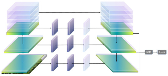
Figure 1.
Proposed net architecture.
The backbone of the network comes from Mobile net [37]. Each flat rectangle in the figure represents the convolutional structure consisting of convolution, bath normalization, and ReLU, where the convolution operation is a depth-wise separable convolution with a kernel of 3 × 3. Green means that the input and output feature maps are of the same size and transparent pink means that a downsampling or upsampling process has occurred. It is downsampling when on the left and upsampling when on the right. The rectangle in the middle of the image indicates the FPN structure, and the specific information is in Section 2.2.
All the convolution structures use Mobile net’s depth-wise convolution. In the depth-separable convolution, the number of channels in the input feature map is first changed to 6 times the original number, and then the output is the target number of channels, and the specific settings are the same as in Mobile net. For the part involving downsampling/upsampling, the resolution of the feature map is changed to 1/2 (downsampling) or 2 times (upsampling) of the original map.
The connection between upsampling and downsampling is made using the FPN structure, and the connection occurs when the feature maps have the same resolution. The connection of different feature maps is simply stacking, and there is no calculation of two feature maps involved. The connection above the FPN is the natural data flow of the model.
3.2. Hough FPN
The Hough transform is a well-known feature identification approach that uses specialized voting rules to identify objects with particular forms. Utilizing the duality of points and lines is its fundamental tenet. The lines in the image space correspond one by one to the points in the parameter space, as illustrated in Figure 2, and the lines in the parameter space correspond to the points in the image space.
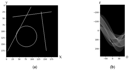
Figure 2.
Image and its matching Hough domain representation. (a) The original image. (b) The representation of image (a) in the Hough domain; the three lines in image (a) are represented as three points in the Hough domain.
For any straight line in any picture :
corresponds to a point in the parameter field , where represents the origin moment of the line and represents the angular direction of the line. Any point in the image is inserted into the picture corresponding to a curve in the parameter domain, the corresponding relationship in the two coordinate systems, the left drawing a straight line, and the right graph exhaustively enumerates the points on each line to get the representation of the Hough domain, and then draws it. The curves corresponding to all the points on the straight lines in the picture will pass through the same point in the Hough domain. As seen in Figure 2b, the point with the highest value in the Hough domain corresponds to the straight line in the main picture if each curve in the Hough domain is viewed as a vote from a pixel of the image.
As is shown in Figure 3, the FPN structure is combined with the Hough transform, which has the advantage of capturing more edge information in the shallow feature maps of the model. The Hough transform is introduced by combining it with the FPN structure to better utilize these edge features. The FPN consists of three identical layers, each composed of three sequential parts: an operator to transform the image domain to the Hough domain, a convolutional layer, and an operator to transform the Hough domain back to the image domain. The input to each layer of the FPN is a downsampled feature map generated with the model, with different scales of 1/2, 1/4, and 1/8 relative to the input image. The FPN outputs a feature map in the image domain, which is connected directly to the upsampling part of the decoder. Only the convolutional layers in the FPN have trainable parameters, and the output feature maps are simply stacked with one of the same size in the decoder part.
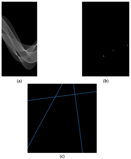
Figure 3.
The process of the Hough fpn: (a) complete the result mapping an image from the image domain to the Hough domain, (b) perform convolution operation on the result from (a) to suppress noise to achieve adaptive point detection, and then (c) map the result in the Hough domain back to the image domain.
The convolution with kernel size = 3 is used in each layer of FPN for the feature map transferred to the parameter domain with the Hough transform, and the padding is specified to guarantee that the feature ’ap’s size is maintained both before and after convolution. The convolution kernel is configured as follows in order to achieve point detection:
The convolutional layer output is activated at the ReLU layer after passing through the Batch Normalization layer, and the outcome is , where is the number of channels in the feature graph, which depends on the number of input channels. According to , the result is mapped back to the image domain, and the size of each pixel in the image is the corresponding value of .
The Hough transform cannot derive the gradient as a voting algorithm. This paper defines the backpropagation functions for the HT module and the IHT module, respectively, in order to achieve gradient backpropagation. The gradient’s backpropagation function for HT is:
where is the bins of the voting result of , that is, the gradient at is defined as the average value of the gradient of each pixel of the corresponding curve in the Hough domain. Similarly, when mapping from the Hough domain to the image domain, the gradient’s backpropagation is:
The gradient at is defined as the average value of each pixel gradient corresponding to the line in the picture domain, where represents the channel, represents the angle, and represents the radius
Various methods for expressing line segments ultimately have an impact on how the Loss function is designed and how the model performs. As a result, this paper uses the tri-points representation proposed by ref. [38]. A line is defined as a midpoint and two endpoints that are presented by the offset from the midpoint. The probability that a pixel is the midpoint of a line segment is predicted using one of the five output feature maps.
This paper uses Focal-Loss as the loss function in the center point classification task because we believe that the foreground line segment is very sparse in comparison to the background. By using Focal-Loss, the model could better utilize the loss produced by positive samples and raise the recognition rate of such samples. The Loss function is expressed as follows:
where is the probability of the correct prediction of a pixel in the output feature map, N is the total number of samples in the picture, γ is used to penalize difficult samples and is often set to 2, and means the loss of center. is the proportional coefficient of the modified positive and negative samples, and its value is expressed as:
In the above equation, represents the number of all samples, in this case the number of all pixels in a predicted image; represents the number of positive samples, in this case the number of midpoints of the labeled line segment; and represents the number of remaining pixels, i.e., the number of pixels in the image that are not positive samples.
There is a regression prediction task for two endpoints in addition to the classification goal of locating the midpoint in the feature map. In the regression prediction, is utilized as the loss function, and its expression is as follows:
where refers to the difference between the predicted value and the true value, and the final loss function of the output map is:
The model also uses the neck structure. The neck structure generates multi-resolution outputs, which are not used as final results but rather as inputs to the NMS algorithm. This method is used because there is a large imbalance between the number of foreground and background samples, and this structure can increase the number of positive samples, making better use of them. In addition, short lines are more accurately predicted in high-resolution feature maps, while long lines are more accurately predicted in low-resolution feature maps. The NMS algorithm combines the results from multiple scales into a single scale to address the discrepancy between the resolutions used during the prediction process.
3.3. Non-Maximum Suppression
The NMS (Non-maximum suppression) algorithm is necessary because it helps to avoid the problem of recognizing a single line as multiple branches in the recognition results, as is shown in Figure 4. NMS ensures that the model detects only one detection result for each item, and the algorithm is only applied to the detection results of the model. The exact procedure of the algorithm is given by Algorithm 1.
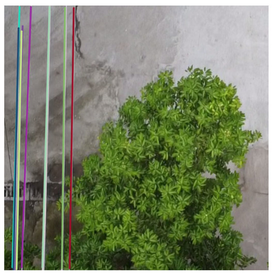
Figure 4.
The model detects one single line for multi-times. The transmission line on the left side of the figure was detected repeatedly.
Algorithm 1 is shown in the Table.
| Algorithm 1 Non-Maximum Suppression |
| Input: is the list of initial detection lines contains corresponding detection scores is the NMS threshold is the midpoint of the line is the midpoint distance threshold begin While do for do if then ; ; new ; ; ifthen ; ; end end return end |
In each round, the algorithm selects the prediction line with the highest score as . Then, for each remaining prediction line , the distance to is determined, where distance is defined as the distance between the two endpoints of to l1. All distances greater than the threshold are kept for the next round. The remaining lines are either suppressed or fused with and will not appear in the next round. Suppression directly deletes the line, while fusion accumulates the midpoint and length of the remaining lines, then averages them to obtain the fused line’s midpoint and length. Finally, the fused line is retained. Fusion and suppression are differentiated by the distance threshold , that is, the distance from the midpoint of the line to the line . This process is repeated until all lines are either retained or suppressed.
4. Results
In this section, the environment including hardware and software is introduced first. Then, give a brief introduction to the dataset we suggested is provided, and the proposed model is compared with other deep learning techniques and conventional methods used in transmission line extraction according to the experimental data. Finally, ablation tests are performed to demonstrate the impact of the suggested Hough-FPN as well as NMS.
4.1. Dataset
Since there are not many datasets currently available for transmission line detection, this paper assembles network images for manual annotation and produces the 1497 RGB images that make up the powerline detection dataset. Figure 5 displays some sample photographs, and the two transmission line endpoints are shown with the dataset. The images are partly taken with drones and partly from the web in a ratio of 2:1. This is for the purpose of improving the generalization of the model, as the diversity in the dataset allows the trained model to be applied to a wide range of scenarios. The parameters regarding the vehicle are as follows: the flight height is 5 m, and all images are finally scaled from 960 × 20 to a size of 512 × 512. In addition to the proposed dataset, the dataset [39] for line segment detection is also used for pre-training in order to enhance the network impact.
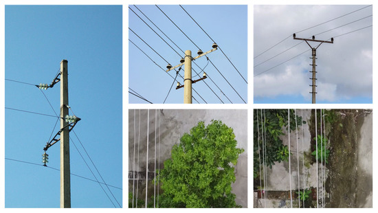
Figure 5.
Samples from the proposed dataset. The dataset includes transmission lines and powerlines, and some of the images are from the Internet. The dataset uses images taken from the drone’s perspective, which can be used for subsequent positioning and other work.
The data set is split into a training set and a test set in the ratio of 9:1 in order to evaluate the performance of the neural network. All the subsequent evaluations are based on the test set.
4.2. Implement Details
4.2.1. Experiment Environment
The hardware environment of the experiment is Nvidia GeForce RTX 3090 Intel i5-12600KF, and the software environment is Ubuntu 20.04 Magi PyTorch 1.8.0 Cudnn 8.2. In order to evaluate the inference speed of the network, the average inference speed of 150 images was calculated.
4.2.2. Training Detail
The initialization for the upsampling portion is bilinear, the initialization for the convolution operation in the Hough transform is (2), and the initialization for the network weight initialization is “kaiming Normal”. This paper uses the SGD (Stochastic Gradient Descent) optimizer, the learning rate decay technique, and the warm-up approach in the area of network training. The initial batch size is 8, and the final batch size 32 after gradient accumulation. A total of 50 epochs are trained on the wireframe dataset during the training phase, and then 150 epochs are trained on the suggested dataset. The training set is enhanced with cropping, rotating, etc.
4.3. Metric
Line segment detection based on a deep learning method can use similar evaluation criteria. First of all, as a geometric figure, the straight line itself can be intuitively represented in the picture, which makes the design of pixel-based evaluation criteria possible. In the transmission line detection task, we believe that the importance of the structural features between line segments is low, and the pixel representation of the final response line detection results is more important. In order to calculate the pixel-based evaluation index, and to facilitate the comparison of the output results of different algorithms, this paper chooses the heat map-based F-score. Next, we briefly introduce the metric and then analyze the results of a variety of algorithms under this metric.
The segment detection performance is frequently measured using the pixel-based F-Score and precision-recall curve, and its primary procedure is as follows:
By picturing the line segment, the endpoint representation of a given line segment creates a heat map. Each pixel is treated independently in order to compare it to the ground truth value. The precision and recall are then calculated based on the results of the matching, and the precision–recall curve is further created.
In this metric, the basic metrics are precision and recall, which are calculated with the following formula:
where TP denotes the proportion of pixels that are present in both the anticipated and actual heat maps, while FP denotes the proportion of pixels that are present exclusively in the predicted heat map and absent from the actual heat map. Recall and precision are two commonly used performance metrics in machine learning and information retrieval. Recall measures how many of the relevant instances in the dataset are identified with the model. A high recall score means that the model is able to identify most of the relevant instances in the dataset. Precision measures how many of the identified instances are relevant to the task at hand. A high precision score means that the model is able to accurately identify relevant instances and is less likely to include irrelevant instances in its results.
Additionally, because the transmission line has a specific width, the ground truth of picture 512 is scaled to 128 before the measurement is calculated in order to better assess the model.
4.4. Comparison with Other Methods
There are numerous techniques for detecting line segments at the moment. It is challenging to compare the conventional method with the method based on deep learning because the concepts are different, and the representation methods of line segments are also different. Based on this assumption, this paper chooses LSD [40] and the probabilistic Hough transform [11] as the method’s output references. The two techniques that are most frequently used in line segment detection are these two. LSD implements gradient-based line feature extraction. By transforming the line segment to the parameter domain, the Hough transform transforms line segment detection into point detection. As for the deep learning method, AFM [30] and DWP [29] are selected for comparison. These methods all select the recommended settings in the paper where the model is proposed, and the code is obtained from open source by the author.
Table 1 displays the summary result, the part marked in red means that the the best performance achieved by the proposed model. The approach this paper proposes had the best result and took the least amount of time. Our method outperforms LSD and HoughP in terms of performance significantly better for the conventional approach. Although our method may not be comparable to LSD and HoughP in terms of inferences per second, the model of this paper is still competitive because it was able to complete inference in real time using GPU. In comparison to previous deep learning techniques, our methods exhibit higher performance and faster inference times with the same or larger input quantity.

Table 1.
Comparison of results between all the algorithms.
First, this paper compares the proposed method with traditional methods. Since traditional methods may not be able to draw the precision–recall curve, this paper draws the kde-graph of precision and recall, as shown in Figure 6. It can be seen that traditional methods may have a slightly better performance in recall, but the proposed method has a significant advantage in precision as well as a tighter distribution and a higher score than the other two methods, which indicates the better and more stable performance of the proposed method.
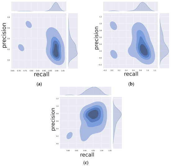
Figure 6.
The kde graph of precision and recall. (a) The kde graph of LSD, it can be seen that the recall is more concentrated and achieved the best recall among the three methods. (b) HoughP is similar to the LSD method, and the distribution of the precision is more dispersed, which means the inner uncertainties in practical application. (c) Our method is closer to the top-right corner in distribution; it could be a little scattered, but it has the best precision score.
As is shown in Figure 7, it is hard for traditional methods to distinguish the target line and the line in the background. With a more complex background, the more the methods are susceptible to noise. It should be noted that, for an image with simple background and foreground objects, such as Figure 7b–d, as can be seen, regardless of splitting one segment into several line segments, the traditional methods showed a great performance. However, in the complex background, a large amount of noise is detected, as can be noted in Figure 7a,d.
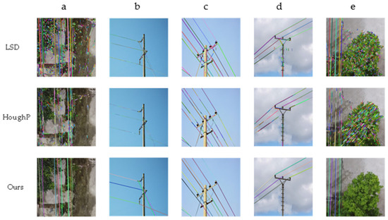
Figure 7.
Comparison of the results of the proposed model with the traditional algorithm (a–e). For simple background cases, such as (b–d), the conventional algorithm produces acceptable results, but there is an inability to perform filtering at the semantic level, such as results in (d), where a portion of the pole is detected as a transmission line, and subsequent screening is required.
To make a fair comparison between our methods and the deep learning-based line segment detector, the model was acquired from the open-source repository and the net was trained using the same techniques as described in Section 4.2.2. For the first round, the model was trained for 50 iterations using the wireframe dataset, and for the second round, 150 iterations using the dataset this paper proposes.
Figure 8 displays the performance of three nets obtained using our dataset. DWP performs well in the low-recall region, but as recall increases, a downward trend develops. AFM has a distribution that is somewhat comparable to DWP, but even with the same recall, AFM is a little lower. Compared to the other two models, the performance of our suggested method is competitive.
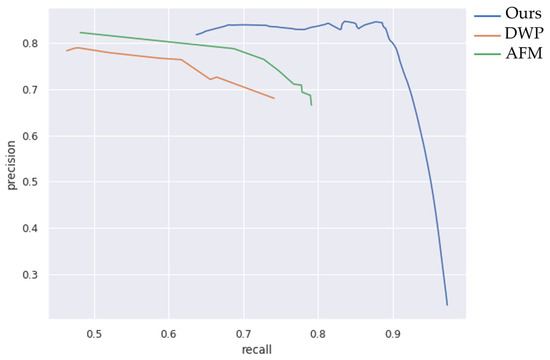
Figure 8.
Precision–recall curve of three models.
Figure 9 shows the result of different models. AFM and DWP are junction-based models, which detect junctions and lines, respectively, and soon afterward combine the junctions and line segments. This may result in the wrong connection, as is shown in Figure 9a,c. The model this paper proposes is based on midpoint detection, with the ability to avoid misconnections. On the other hand, the proposed Hough FPN structure is more advantageous in long straight-line detection, which is reflected in the suppression of noise. As is shown in Figure 9, with the most complex background, our methods detect the least noise.
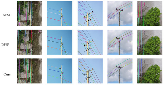
Figure 9.
Comparison of the results of our model and the other two-line detector based on deep learning.
The model proposed in this paper can obtain better line segment detection results and also has a better performance for the detection of long lines.
4.5. Ablation Study
In this section, a series of ablation experiments were conducted to analyze the proposed method.
First, this paper compares the output of the model with and without the Hough FPN and discusses how the training speed can be accelerated. As shown in Figure 10, the loss of the model without the Hough FPN is higher than the loss of the model with the Hough FPN throughout the training process. Therefore, this paper concludes that the proposed FPN structure can facilitate the training acceleration.
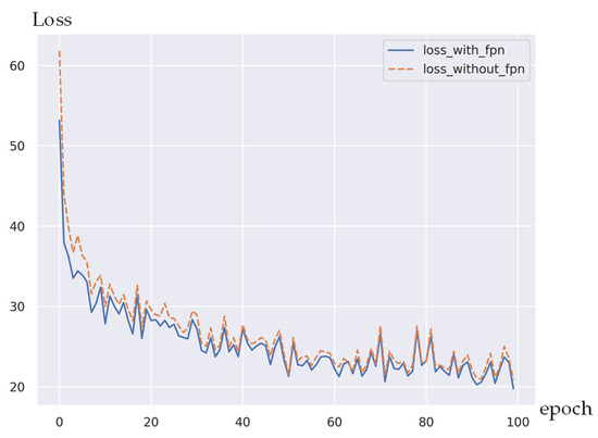
Figure 10.
Comparison between the speed of loss reduction with and without Hough FPN.
Next, this paper discusses the improvement in the proposed FPN structure in terms of the performance of the model. For a fair comparison, the NMS algorithm is not applied in the experiment. As shown in Figure 11, it can be observed that the introduction of this structure can better perceive the straight-line features in the image and suppress the interference of noise in the environment to a certain extent. It is speculated that this is because the introduction of Hough FPN increases the proportion of line segment features, thereby reducing the score of difficult backgrounds in the training process and finally optimizing the result. It can also be noted that the introduction of Hough FPN can reduce false detections. In Figure 11, the model without Hough FPN detected a line that does not exist. This paper speculates that the reason for this issue is that the model pays more attention to the texture rather than the line structure in the image, which can be alleviated using Hough FPN. In summary, this paper thinks that the Hough FPN can make the model pay more attention to the line structure rather than the texture.

Figure 11.
Comparison of performance in complex background performed using the models with or without Hough FPN.
The effect of introducing non-maximum suppression (NMS) on the model performance is also discussed in this paper. The model was based on detecting the midpoint of the line and taking multi-resolution feature maps as outputs, which resulted in frequent multiple detections of a single line. As shown in Figure 12, introducing NMS could eliminate redundant midpoints and merge adjacent lines into one line segment. For example, in Figure 12, the model without NMS detected a line segment multiple times, while the model with NMS identified false detections by measuring the distance between line segments and merging them into a single line. As can be seen from the data in Figure 13, the use of FPN layers obtains a larger precision with the same recall, which means that the introduction of FPN leads to more accurate line segment predictions. The introduction of the NMS algorithm reduces the model’s performance to some extent, as shown by the sharp drop in the performance of the model after the recall is greater than a certain value. This is mainly because the NMS algorithm removes or fuses some line segments, and the reduction in line segments lead to the reduction in pixel overlap, which in turn leads to the decrease in precision for the same recall. However, as can be seen in the actual results, the NMS algorithm can filter out the repeatedly detected line segments. We believe that guaranteeing the uniqueness of transmission line detection in the image is more important for subsequent tasks such as localization or flying along a straight line than for the evaluation results.
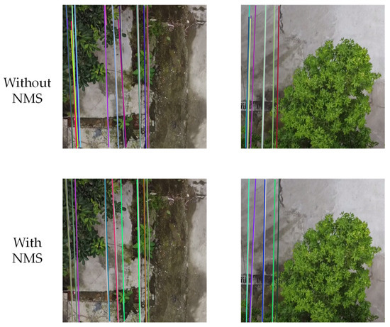
Figure 12.
Comparison of the result before and after NMS.
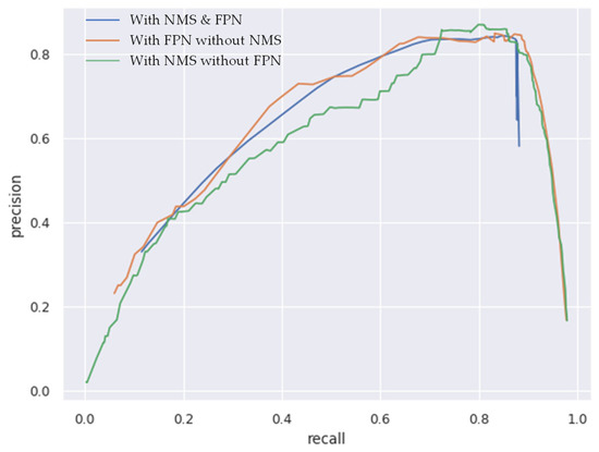
Figure 13.
Comparison of the pre–rec curve with or without FPN and NMS.
5. Discussion
A novel method for detecting transmission lines in images is proposed, which is based on the texture features of the images and incorporates the structural information of the images. This deep learning-based approach has several benefits over traditional manual detection, such as high accuracy, semantic information extraction, and avoiding multiple detections of the same line. The following paragraph will discuss some challenges and improvements of this method.
A limitation of the proposed method is that it assumes transmission lines to be long and straight, while in reality, they may be curved or irregular. The method can handle some degree of bending in the transmission lines, as shown in the results and analyses, but it fails to detect them in some extreme cases, such as in Figure 14.
Figure 14.
Curved transmission lines.
However, the model still faces some challenges in actual use. First, the model relies on the acceleration of the GPU, which may not be compatible with the arithmetic platform and power reserve of the UAV device. Therefore, there are still some technical gaps in real-time positioning and navigation in real situations. Second, due to the characteristics of deep learning, the model needs to re-establish the dataset and train in different scenarios. Moreover, as the device is often used outdoors, environmental changes caused by the seasons are also one of the problems to be considered. In practice, another issue that transmission line detection face is the presence of large obstacles, particularly large linear ones. In the experiments carried out so far, the network often encounters situations where the edges of windows, cracks in the ground, etc., are detected as transmission lines. In response to these problems, this paper has preliminary solutions to discuss.
- Selective training for real scenarios. In order to increase the generalization capability of the model, a large number of network images are introduced in addition to the proposed dataset. In real scenarios, the model may not need to recognize multiple styles of transmission lines, and more effective obstacle rejection may be achieved with reducing the generalization capability.
- This can be accomplished with establishing negative samples. To improve the obstacle rejection effect, we design the Loss function and mark the obstacles in the dataset as negative samples.
The detection of transmission lines alone is not sufficient for autonomous UAV localization. It also requires the computation of line segment descriptors and the construction of a feature dictionary under the scene to determine inter-frame relationships. The LBD operator can be applied in the situation where the UAV is located to match line segments between two frames, and reprojection errors can be used to estimate inter-frame poses. Furthermore, the computational effort can be reduced with the assumption of linear uniform motion of adjacent frames. These are future research directions.
6. Conclusions
This research proposes an end-to-end transmission line detection model based on the study and synthesis of the features of transmission lines in images. The model uses the three-point approach to characterize straight lines in images and develops a line segment extraction network to capture the line segments. The model also introduces the Hough FPN structure, which is designed for the transmission line, which often appears as a long straight line across the entire image. The Hough FPN structure enables the model to better utilize the edge features of the shallow layer of the network and also accelerates the model training. Moreover, the model applies a corresponding NMS algorithm to address the problem of multiple detections of a single straight line that may occur in the network detection results. The model achieves improved performance and lays the foundation for potential future high-level tasks. The model has advantages over traditional methods, such as higher accuracy, no segmentation of line segments, and the semantic level of the extracted lines. The model extracts line segments based on endpoints, which can provide line features that can be utilized for localization by UAVs and other devices, enabling them to achieve self-navigation and localization to a certain extent and consume less personnel. The model has a wide range of application possibilities.
Author Contributions
Conceptualization, C.G.; Methodology, C.G.; Software, J.H. (Jingwei Hu); Investigation, J.H. (Jing He); Project administration, J.H. (Jingwei Hu). All authors have read and agreed to the published version of the manuscript.
Funding
This research received no external funding.
Data Availability Statement
The data presented in this study are available on request from the corresponding author. The data are not publicly available due to privacy. And the model this paper proposed can be found here: https://github.com/iifeve/power_line_detection (accessed on 1 March 2023).
Conflicts of Interest
The authors declare no conflict of interest.
References
- Nasseri, M.H.; Moradi, H.; Nasiri, S.M.; Hosseini, R. Power Line Detection and Tracking Using Hough Transform and Particle Filter. In Proceedings of the 2018 6th RSI International Conference on Robotics and Mechatronics (IcRoM), Tehran, Iran, 23–25 October 2018. [Google Scholar]
- Hough, P.V.C. Method and Means for Recognizing Complex Patterns. U.S. Patent 3,069,654, 18 December 1962. [Google Scholar]
- Zhang, X.; Zhang, L.; Li, D. Transmission line abnormal target detection based on machine learning yolo v3. In Proceedings of the 2019 International Conference on Advanced Mechatronic Systems (ICAMechS), Kusatsu, Japan, 26–28 August 2019; pp. 344–348. [Google Scholar]
- Bao, W.; Ren, Y.; Wang, N.; Hu, G.; Yang, X. Detection of Abnormal Vibration Dampers on Transmission Lines in UAV Remote Sensing Images with PMA-YOLO. Remote Sens. 2021, 13, 4134. [Google Scholar] [CrossRef]
- Redmon, J.; Farhadi, A. Yolov3: An Incremental Improvement. arXiv 2018, arXiv:1804.02767. [Google Scholar]
- Zhai, Y.; Yang, X.; Wang, Q.; Zhao, Z.; Zhao, W. Hybrid knowledge R-CNN for transmission line multifitting detection. IEEE Trans. Instrum. Meas. 2021, 70, 1–12. [Google Scholar] [CrossRef]
- Vemula, S.; Frye, M. Mask R-CNN powerline detector: A deep learning approach with applications to a UAV. In Proceedings of the 2020 AIAA/IEEE 39th Digital Avionics Systems Conference (DASC), San Antonio, TX, USA, 11–15 October 2020; pp. 1–6. [Google Scholar]
- Liu, B.; Liu, H.; Yuan, J. Lane line detection based on mask R-CNN. In Proceedings of the 3rd International Conference on Mechatronics Engineering and Information Technology (ICMEIT 2019), Dalian, China, 29–30 March 2019; Atlantis Press: Paris, France, 2019; pp. 696–699. [Google Scholar]
- Duda, R.O.; Hart, P.E. Use of the Hough transformation to detect lines and curves in pictures. Commun. ACM 1972, 15, 11–15. [Google Scholar] [CrossRef]
- Illingworth, J.; Kittler, J. The adaptive Hough transform. IEEE Trans. Pattern Anal. Mach. Intell. 1987, 5, 690–698. [Google Scholar] [CrossRef] [PubMed]
- Kiryati, N.; Eldar, Y.; Bruckstein, A.M. A probabilistic Hough transform. Pattern Recognit. 1991, 24, 303–316. [Google Scholar] [CrossRef]
- O’gorman, F.; Clowes, M.B. Finding picture edges through collinearity of feature points. IEEE Trans. Comput. 1976, 25, 449–456. [Google Scholar] [CrossRef]
- Galamhos, C.; Matas, J.; Kittler, J. Progressive probabilistic Hough transform for line detection. In Proceedings of the 1999 IEEE Computer Society Conference on Computer Vision and Pattern Recognition (Cat. No PR00149), Fort Collins, CO, USA, 23–25 June 1999; Volume 1, pp. 554–560. [Google Scholar]
- Zhou, G.; Yuan, J.; Yen, I.L.; Bastani, F. Robust real-time UAV based power line detection and tracking. In Proceedings of the 2016 IEEE International Conference on Image Processing (ICIP), Phoenix, AZ, USA, 25–28 September 2016; pp. 744–748. [Google Scholar]
- Gerke, M.; Seibold, P. Visual inspection of power lines by UAS. In Proceedings of the 2014 International Conference and Exposition on Electrical and Power Engineering (EPE), Iasi, Romania, 16–18 October 2014; pp. 1077–1082. [Google Scholar]
- Jones, D.; Golightly, I.; Roberts, J.; Usher, K. Modeling and control of a robotic power line inspection vehicle. In Proceedings of the 2006 IEEE Conference on Computer Aided Control System Design 2006 IEEE International Conference on Control Applications, 2006 IEEE International Symposium on Intelligent Control, Munich, Germany, 4–6 October 2006; pp. 632–637. [Google Scholar]
- Fernandes, L.A.F.; Oliveira, M.M. Real-time line detection through an improved Hough transform voting scheme. Pattern Recognit. 2008, 41, 299–314. [Google Scholar] [CrossRef]
- Limberger, F.A.; Oliveira, M.M. Real-time detection of planar regions in unorganized point clouds. Pattern Recognit. 2015, 48, 2043–2053. [Google Scholar] [CrossRef]
- Yacoub, S.B.; Jolion, J.M. Hierarchical line extraction. IEE Proc.-Vis. Image Signal Process. 1995, 142, 7–14. [Google Scholar] [CrossRef]
- Princen, J.; Illingworth, J.; Kittler, J. A hierarchical approach to line extraction based on the Hough transform. Comput. Vis. Graph. Image Process. 1990, 52, 57–77. [Google Scholar] [CrossRef]
- Aggarwal, N.; Karl, W.C. Line detection in images through regularized Hough transform. IEEE Trans. Image Process. 2006, 15, 582–591. [Google Scholar] [CrossRef] [PubMed]
- Min, J.; Lee, J.; Ponce, J.; Cho, M. Hyperpixel flow: Semantic correspondence with multi-layer neural features. In Proceedings of the IEEE/CVF International Conference on Computer Vision, Seoul, Korea, 27 October–2 November 2019; pp. 3395–3404. [Google Scholar]
- Qi, C.R.; Litany, O.; He, K.; Guibas, L.J. Deep hough voting for 3d object detection in point clouds. In Proceedings of the IEEE/CVF International Conference on Computer Vision, Seoul, Korea, 27 October–2 November 2019; pp. 9277–9286. [Google Scholar]
- Lin, Y.; Pintea, S.L.; van Gemert, J.C. Deep hough-transform line priors. In Proceedings of the Computer Vision–ECCV 2020: 16th European Conference, Glasgow, UK, 23–28 August 2020; Springer International Publishing: Cham, Switzerland, 2020; pp. 323–340. [Google Scholar]
- Redmon, J.; Divvala, S.; Girshick, R.; Farhadi, A. You only look once: Unified, real-time object detection. In Proceedings of the IEEE Conference on Computer Vision and Pattern Recognition, Las Vegas, NV, USA, 26 June–1 July 2016; pp. 779–788. [Google Scholar]
- Law, H.; Deng, J. Cornernet: Detecting objects as paired keypoints. In Proceedings of the European Conference on Computer Vision (ECCV), Munich, Germany, 8–14 September 2018; pp. 734–750. [Google Scholar]
- Ren, S.; He, K.; Girshick, R.; Sun, J. Faster r-cnn: Towards real-time object detection with region proposal networks. Adv. Neural Inf. Process. Syst. 2015, 28. [Google Scholar] [CrossRef] [PubMed]
- Wang, K.; Liew, J.H.; Zou, Y.; Zhou, D.; Feng, J. Panet: Few-shot image semantic segmentation with prototype alignment. In Proceedings of the IEEE/CVF International Conference on Computer Vision, Seoul, Korea, 27 October–2 November 2019; pp. 9197–9206. [Google Scholar]
- Huang, K.; Wang, Y.; Zhou, Z.; Ding, T.; Gao, S.; Ma, Y. Learning to parse wireframes in images of man-made environments. In Proceedings of the IEEE Conference on Computer Vision and Pattern Recognition, Salt Lake City, UT, USA, 18–23 June 2018; pp. 626–635. [Google Scholar]
- Xue, N.; Bai, S.; Wang, F.; Xia, G.S.; Wu, T.; Zhang, L. Learning attraction field representation for robust line segment detection. In Proceedings of the IEEE/CVF Conference on Computer Vision and Pattern Recognition, Long Beach, CA, USA, 15–20 June 2019; pp. 1595–1603. [Google Scholar]
- Siranec, M.; Höger, M.; Otcenasova, A. Advanced power line diagnostics using point cloud data—Possible applications and limits. Remote Sens. 2021, 13, 1880. [Google Scholar] [CrossRef]
- Awrangjeb, M. Extraction of power line pylons and wires using airborne lidar data at different height levels. Remote Sens. 2019, 11, 1798. [Google Scholar] [CrossRef]
- Pan, C.; Cao, X.; Wu, D. Power line detection via background noise removal. In Proceedings of the 2016 IEEE Global Conference on Signal and Information Processing (GlobalSIP), Washington, DC, USA, 7–9 December 2016; pp. 871–875. [Google Scholar]
- Benlıgıray, B.; Gerek, Ö.N. Visualization of power lines recognized in aerial images using deep learning. In Proceedings of the 2018 26th Signal Processing and Communications Applications Conference (SIU), Izmir, Turkey, 2–5 May 2018; pp. 1–4. [Google Scholar]
- Zhu, K.; Xu, C.; Wei, Y.; Cai, G. Fast-PLDN: Fast power line detection network. J. Real-Time Image Process. 2022, 19, 3–13. [Google Scholar] [CrossRef]
- Dai, Z.; Yi, J.; Zhang, H.; Wang, D.; Huang, X.; Ma, C. CODNet: A Center and Orientation Detection Network for Power Line Following Navigation. IEEE Geosci. Remote Sens. Lett. 2021, 19, 1–5. [Google Scholar] [CrossRef]
- Sandler, M.; Howard, A.; Zhu, M.; Zhmoginov, A.; Chen, L.C. Mobilenetv2: Inverted residuals and linear bottlenecks. In Proceedings of the IEEE Conference on Computer Vision and Pattern Recognition, Salt Lake City, UT, USA, 18–23 June 2018; pp. 4510–4520. [Google Scholar]
- Huang, S.; Qin, F.; Xiong, P.; Ding, N.; He, Y.; Liu, X. TP-LSD: Tri-points based line segment detector. In European Conference on Computer Vision; Springer: Cham, Switzerland, 2020; pp. 770–785. [Google Scholar]
- Zhou, Y.; Qi, H.; Ma, Y. End-to-end wireframe parsing. In Proceedings of the IEEE/CVF International Conference on Computer Vision, Seoul, Korea, 27 October–2 November 2019; pp. 962–971. [Google Scholar]
- Von Gioi, R.G.; Jakubowicz, J.; Morel, J.M.; Randall, G. LSD: A line segment detector. Image Process. Line 2012, 2, 35–55. [Google Scholar] [CrossRef]


Disclaimer/Publisher’s Note: The statements, opinions and data contained in all publications are solely those of the individual author(s) and contributor(s) and not of MDPI and/or the editor(s). MDPI and/or the editor(s) disclaim responsibility for any injury to people or property resulting from any ideas, methods, instructions or products referred to in the content. |
© 2023 by the authors. Licensee MDPI, Basel, Switzerland. This article is an open access article distributed under the terms and conditions of the Creative Commons Attribution (CC BY) license (https://creativecommons.org/licenses/by/4.0/).