1. Introduction
Unmanned aerial vehicles (UAVs) play a vital role in remote sensing and are used as mobile measuring and monitoring devices, e.g., in precision agriculture (for observing the inter- and intra-variability of crops or for detecting pests) or in infrastructure inspection (for detecting defects or degradation such as corrosion). Many applications require both high-resolution 3D spatial and multi-band spectral data in order to infer the characteristics and behavior of various (living) materials. However, few hardware systems collect high-resolution 3D spatial and multiband spectral information simultaneously in one integrated airborne solution. In this work, we bridge the gap between LiDAR (Light Detection and Ranging) scanning and traditional imaging (such as RGB, hyperspectral, and thermal cameras), two complementary technologies. Our sensor fusion pipeline allows spectral, spatial and thermal data to be extracted and related to variables relevant to specific applications.
One of the application domains that benefit from multimodal data is infrastructure inspection or damage assessment. For example, in the case of wind farms, spatial data from LiDAR aids in the detection of concrete rot in the pedestals of the wind turbines, whereas the hyperspectral data is very well suited to detect corrosion on the blades. Similarly, in large-scale PV (photovoltaic) power plants, thermal data are used for the detection of hotspots, whereas hyperspectral images are very well suited to detect the erosion of the anti-reflectance coating. Other examples are bridges (concrete rot and coating delamination), transmission towers (corrosion and structural damages), or high-voltage power lines (overheating and sagging). A second application domain is precision agriculture and forestry. In the case of precision agriculture, hyperspectral imaging provides insight into the spectral reflectance of the crop, which may reveal information about the plant health, e.g., to infer nutrient status or the presence of biotic or abiotic stress [
1]. LiDAR data, on the other hand, provides information on the height or growth vigor of the crop. For example, parts of the crop may have stunted growth due to a lack of sunlight or overgrowing weeds. Similarly, hyperspectral imaging provides insights into the health and biodiversity of forests, their composition in terms of tree species, the presence of different types of stress (e.g., from beetles) and so on. The LiDAR data, in turn, provide information on the forest structure characteristics, including basal area, stem volume, dominant height, and biomass [
2].
The combination of LiDAR and traditional imaging has not yet been fully exploited in the scientific literature because not all required techniques on calibration, registration, corrections, optimal scanning strategies, etc., are fully optimized. As such, the generation of multispectral point clouds from UAV platforms remains imprecise or suboptimal to date. In our research, we aim at making the most of both LiDAR and traditional imaging by developing a fully synchronized multimodal UAV payload and an associated processing pipeline able to produce georeferenced multispectral point clouds with subcentimeter accuracy. To that end, we have improved several state-of-the-art algorithms in the field of multimodal calibration, point cloud registration, spatial corrections, and optimal scanning strategies. More specifically, we propose an optimized self-localization and mapping algorithm that combines advanced point cloud registration with photogrammetric bundle adjustment and the output of a precision GNSS/INS (Global Navigation Satellite System/Inertial Navigation System). The latter is able to generate high-frequency navigation outputs with centimeter accuracy. However, due to the highly dynamic movements and occasional under-measurements, the accuracy can be as poor as five centimeters, causing the generated point clouds to suffer from distortions or discrepancies, especially when the UAV turns abruptly at the end of the flight line. In those cases, our LiDAR registration algorithm is able to compensate for the abrupt movements and under-measurements of the INS, thereby preventing severe distortion.
This paper is organized as follows. In
Section 2, the related work is extensively described, in terms of both technology and applications. We discuss how our approach fits within their methodological frameworks, and equally importantly, where it deviates, allowing us to overcome inherent limitations. In
Section 3, the hardware set-up and the pipeline are described, including all contributions. In
Section 4, the experiments and results of the pipeline are discussed. Finally,
Section 5 contains the main conclusions of this research.
2. Related Work
On self-localization and mapping through the fusion of inertial, LiDAR, and visual data, several papers have been published in recent years. Many of these works were conducted in the context of autonomous driving, for which computation time is crucial. In 2015, Zhang et al. [
3] proposed their Visual–LiDAR odometry and mapping, better known as V-LOAM, which has been the best method for years according to the well-known KITTI odometry benchmark [
4], until it was beaten by SOFT2 [
5] in early 2022. Other well-performing and fast LiDAR–Visual SLAM methods are LIMO (LiDAR-monocular SLAM) [
6], DVL-SLAM [
7] and the method presented by Wang et al. [
8].
A common criticism regarding the KITTI benchmark, which is focused on autonomous driving, is that researchers tend to over-optimize to the specifications of that particular dataset, which limits the generality of the proposed methods. For example, in the case of a moving car, there are hardly any rotations around the roll axis and the “short-term” dynamics are very limited. In this paper, we deal with scenes and circumstances that are a lot more challenging in nature compared to the KITTI dataset. Since we consider data acquired from UAVs, all LiDAR points are captured from a relatively far distance (i.e., the height of the UAV flight trajectory), and many LiDAR points are sampled on a relatively flat ground plane (which could lead to a degenerate situation). Additionally, the drone is subject to many highly dynamic micro-movements, and often, the scene lacks structural elements or consists of large regions with a lot of repetitiveness (e.g., crops). On the other hand, since we focus on outdoor environments, we can use GNSS data to compensate for drift and to initialize self-localization prior to the actual point cloud registration. In addition, our use case does not require real-time execution since the final output (multispectral point clouds rather than the odometry itself) is mainly used for offline analysis.
The literature on the fusion of inertial, LiDAR, and visual data for UAV applications is much scarcer. Obviously, it is a lot harder to build multisensor payloads that fit under a UAV and do not surpass its maximum payload weight. Nagai et al. [
9] pioneered building a multisensor UAV platform, consisting of two regular RGB cameras, two infrared cameras, a SICK laser scanner, a GNSS receiver and an inexpensive IMU. They integrated the GNSS and IMU data using Kalman filtering to obtain position and attitude estimates that guide the search for tie points used to register the image data through bundle block adjustment (BBA). The output of the BBA, in turn, aids the Kalman filtering by initializing the position and attitude in the next step in order to acquire a much more accurate trajectory. The final trajectory is eventually used to register the laser range data and to obtain a digital surface model, for which the authors report an average error of approximately 10 to 30 cm. A major difference with our work is that we increase the accuracy of the position and attitude data from the INS using a dedicated point cloud registration technique, which leads to fewer (visual) artifacts but also contributes to the overall accuracy. Consequently, we obtain point clouds or digital surface models that are one order of magnitude more accurate.
More recently, Qian et al. [
10] presented a multisensor UAV payload and SLAM algorithm that is based on the fusion of Velodyne LiDAR data and RGB imagery. More specifically, they extract line and plane features from the LiDAR data and use them to compute the relative pose between consecutive frames in an ICP-based manner. Afterward, the relative pose is refined by combining it with visual odometry computed from the images. For that purpose, they use the relative pose error as a prior and subsequently minimize a photometric error. The work of Qian et al. is similar to ours in the sense that we also use the poses computed by LiDAR-based odometry (along with the output of the GNSS/IMU) as a prior for image-based reconstruction. However, we conduct a full 3D reconstruction using the image data (based on bundle adjustment) instead of limiting ourselves to visual odometry. The latter is justified, as we focus more on the overall mapping accuracy instead of the computation time. Note that our LiDAR and GNSS/INS-based self-localization itself is running in real-time. Finally, compared to [
10], our approach allows fusing data from different imaging modalities such as a multispectral, hyperspectral or thermal camera, which usually have a limited and different spatial resolution.
Haala et al. [
11,
12] presented another multisensor UAV platform consisting of a Riegl VUX-1 LiDAR Scanner, Applanix AP 20 GNSS/IMU-unit and Phase One iXM-RS150F camera. Based on the foundations laid in the previous work of Cramer et al. [
13], the authors apply hybrid georeferencing, integrating photogrammetric bundle block adjustment with direct georeferencing of LiDAR point clouds. They demonstrate that 3D point cloud accuracies of subcentimeter level can be achieved. This is realized by a joint orientation of laser scans and images in a hybrid adjustment framework, which enables accuracies corresponding to the ground sampling distance (GSD) of the captured imagery. Although the work of [
11] has some similarities with ours, the main difference is that it does not use a dedicated point-cloud registration algorithm to improve the position and attitude estimates of the GNSS, nor does it integrate data from multispectral or thermal cameras.
Bultman et al. [
14] propose a UAV system for real-time semantic fusion and segmentation of multiple sensor modalities. For visual perception, their UAV carries two Intel RealSense D455 RGB-D cameras mounted on top of each other to increase the vertical field-of-view and a FLIR thermal camera to alleviate person detection in search-and-rescue scenarios. For 3D perception and odometry, they additionally integrated an Ouster LiDAR scanner on their UAV. Unlike our work, the authors do not focus on the alignment of the scans and images, nor do they focus on the SLAM algorithm. They mention the multi-view aggregation of point clouds, but for that purpose, they use voxel hashing to save memory, as their main use case is real-time semantic segmentation. As a result, the resolution of the obtained map is low.
Besides the actual mapping, other problems need to be solved, one of them being the calibration between the different sensors. In this work, we adopt late fusion by precisely merging the different orthophotos from the cameras with the point cloud obtained by the LiDAR scanner. In the future, we plan to integrate a more tight coupling between the point cloud registration and photometric bundle adjustment, for which an accurate calibration between the LiDAR and cameras would be required. One such method is CalibRCNN, presented by Shi et al. [
15], which uses a Recurrent Convolutional Neural Network (RCNN) to infer the six-degrees-of-freedom rigid body transformation between the two modalities. For our current approach, only the calibration of the GNSS/INS device and the other sensors has to be estimated, which is described in detail in
Section 3.3.
Plenty of other research relies on data captured from a multi-sensor UAV payload. Most of those publications focus more on the specific application rather than on the technical challenges related to the mapping and fusion of multimodal data. As mentioned in the introduction, a lot of this research is conducted in the context of agriculture or forestry. For example, Zhou et al. [
16] used a DJI M600 UAV carrying a Pika L hyperspectral camera and an LR1601-IRIS LiDAR scanner for the purpose of detecting emerald ash borer (EAB) stress in ash. In [
17], the authors used the same setup to detect pine wilt disease at the tree level. Finally, the authors of [
18] fused UAV-based hyperspectral images and LiDAR data to detect pine shoot beetle. For more examples, we refer to the literature review by Maes and Steppe [
1].
3. Materials and Methods
3.1. Sensors
As shown in
Figure 1, our multisensor payload consists of an Ouster OS1-128 LiDAR scanner, a Micasense RedEdge-MX Dual camera system, a Teax ThermalCapture 2.0 thermal camera with an integrated FLIR Tau 2 sensor, and an inertial navigation system (INS) aided by an SBG Quanta GNSS (with a dual antenna system). The payload is controlled by an NVIDIA Jetson Xavier NX.
The Quanta has a roll/pitch accuracy of 0.015°, a heading accuracy of 0.035°, and a position accuracy of around 1 cm in post-processing (PPK). The Micasense cameras have an image resolution of 1280 × 960 and a field of view of 47.2° horizontally and 35.4° vertically. Consequently, they have a ground sampling distance (GSD) of 8 cm per pixel at a height of 120 m or 1.33 cm at a height of 20 m. Together, they cover 10 different wavelengths in the range between 444 nm and 842 nm. Every second, an image is captured for each band. The Teax ThermalCapture 2.0 has a 640 × 480 resolution and operates at 30 or 60 Hz. With a 13 mm lens and 17 μm pixel pitch, it has a GSD of 2.6 cm/pixel at a height of 20 m.
Finally, the Ouster LiDAR scanner has 128 scan lines, a horizontal FOV of 360°, and a vertical FOV of 45°. It has a precision of 1 to 3 cm and operates in the 865 nm wavelength. Furthermore, it supports three different scanning configurations (horizontal resolution × rotation rate): 1024 × 10, 1024 × 20, and 2048 × 10. The GSD depends on the rotation rate and horizontal resolution and is different in the vertical and horizontal directions. For the optimal setup of the LiDAR sensor for UAV swath surveys, we refer the interested reader to [
19]. The main specifications of the sensors are summarized in
Table 1.
3.2. Synchronization
The Ouster scanner is synchronized with the Quanta INS by time-stamping every firing of laser beams. The scanner supports three clock sources: (1) internal clock, (2) external PPS (Pulse Per Second) sync pulse from a GNSS/INS, and (3) external Precision Time Protocol (PTP). In our case, we adopt the PPS time synchronization to query the GNSS time from the Quanta and write it in the data frame of the LiDAR scan. In other words, every time the Ouster scanner fires 128 laser beams, a GNSS timestamp is saved in its data frame. Depending on the configuration, either 1024 (possible at a rotation rate of 10 Hz or 20 Hz) or 2048 (in case of 10 Hz rotation rate) timestamps are saved. The time precision, i.e., the minimum increment for the time, is 10 ns. The Micasense and the ThermalCapture cameras each have their dedicated GNSS receiver, and the GNSS timestamp is written in the metadata of the acquired images. By matching the timestamps of the cameras with the INS output from the Quanta, high-precision position and attitude information can be fetched for every image.
3.3. Calibration of the Sensors
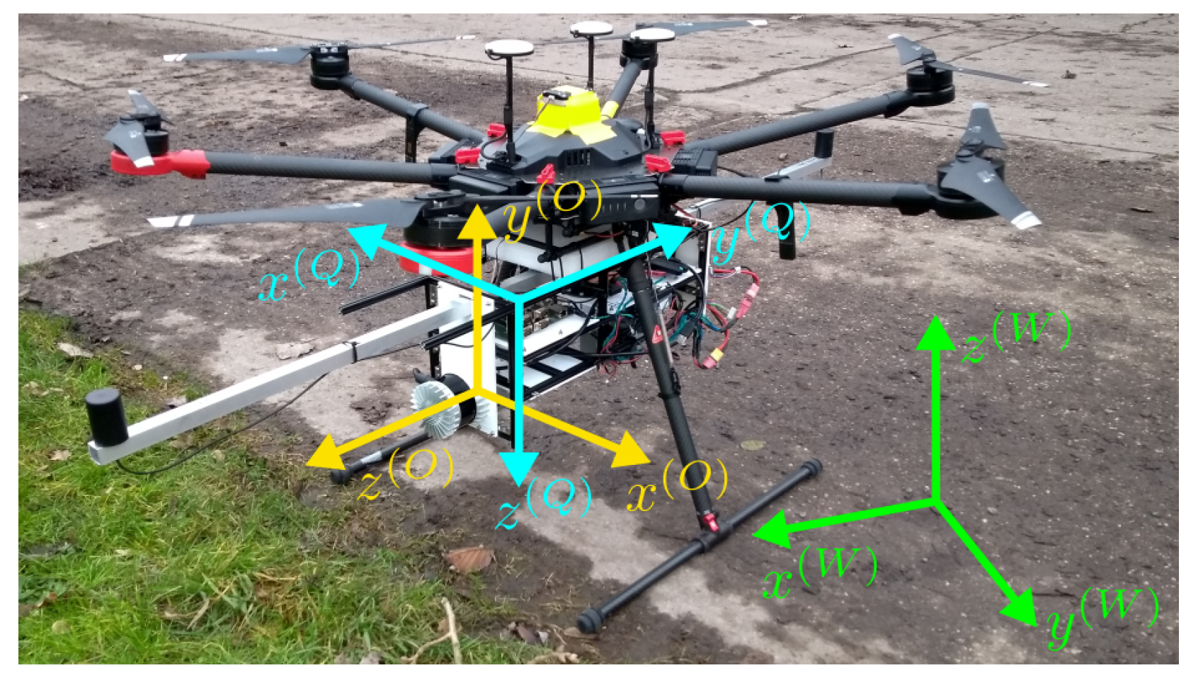
For the extrinsic calibration between the different sensors, we look for the rigid body transformations mapping each sensor’s coordinate frame to the Quanta GNSS’s frame. Due to the right-angled nature of our sensor rig and mounting configurations, specifying the rotational parts is straightforward. For example, in
Figure 2, the LiDAR’s
-direction coincides with the UAV’s forward direction, which is, in our mounting configuration, the Quanta’s negative
-direction. Similarly, all other sensor axis directions coincide with one of the Quanta’s axis directions. If we intentionally mount a sensor at an oblique angle, we can specify the rotation via Euler angles in a convenient order so that two Euler angles are a multiple of 90° and the third is our intended oblique angle (which we usually know in advance, or we can simply measure if not). The translational parts of the transformation matrices, i.e., the location of the sensor frame’s origin in local Quanta coordinates, can also be measured using a simple ruler.
However, unknown deviations from the right-angled nature of the mounting can occur, for example, if some screws are fixed tighter than others. Therefore, we will use the calibrations described above as the initialization for an optimization method, which will refine the calibration parameters. For this purpose, we make use of a 97 cm by 96 cm calibration plate, shown in
Figure 3. As can be seen, it has a 2 × 2 black-and-white checkerboard pattern, allowing us to use standard (grayscale) techniques to detect it in the multispectral images. Since we actively cool the white parts with ice (and the black parts should also become warmer than the surrounding through reflecting sunlight less), the same can be said for the thermal images. Together with a calibration flight, where we fly over the plate at different heights and at different angles, and with ground measurement of the plate center’s location, we can optimize the external camera calibration parameters.
To detect the calibration plate in the LiDAR data, we found intensity/reflectivity information to be insufficient, and we therefore placed the plate on a table approximately 1.5 m high. This allowed us to separate the plate from the ground directly from the 3D LiDAR information, at least if the calibration error remains within reasonable margins. This would not be the case if we used all scans from the entire calibration flight. However, if we only take scans on the same flight line, where the UAV’s orientation is approximately constant, we are indeed able to segment out the calibration plate. For this purpose, we found a simple -threshold (made somewhat adaptive by declaring it in terms of a -quantile) to work sufficiently well. To find the plate center in the data, we used a componentwise median to be more robust to noise. Using the distance between the data-detected plate center and its ground truth location as a loss function, we can improve the calibration parameters using gradient-descent-based techniques by going through the different flight lines multiple times.
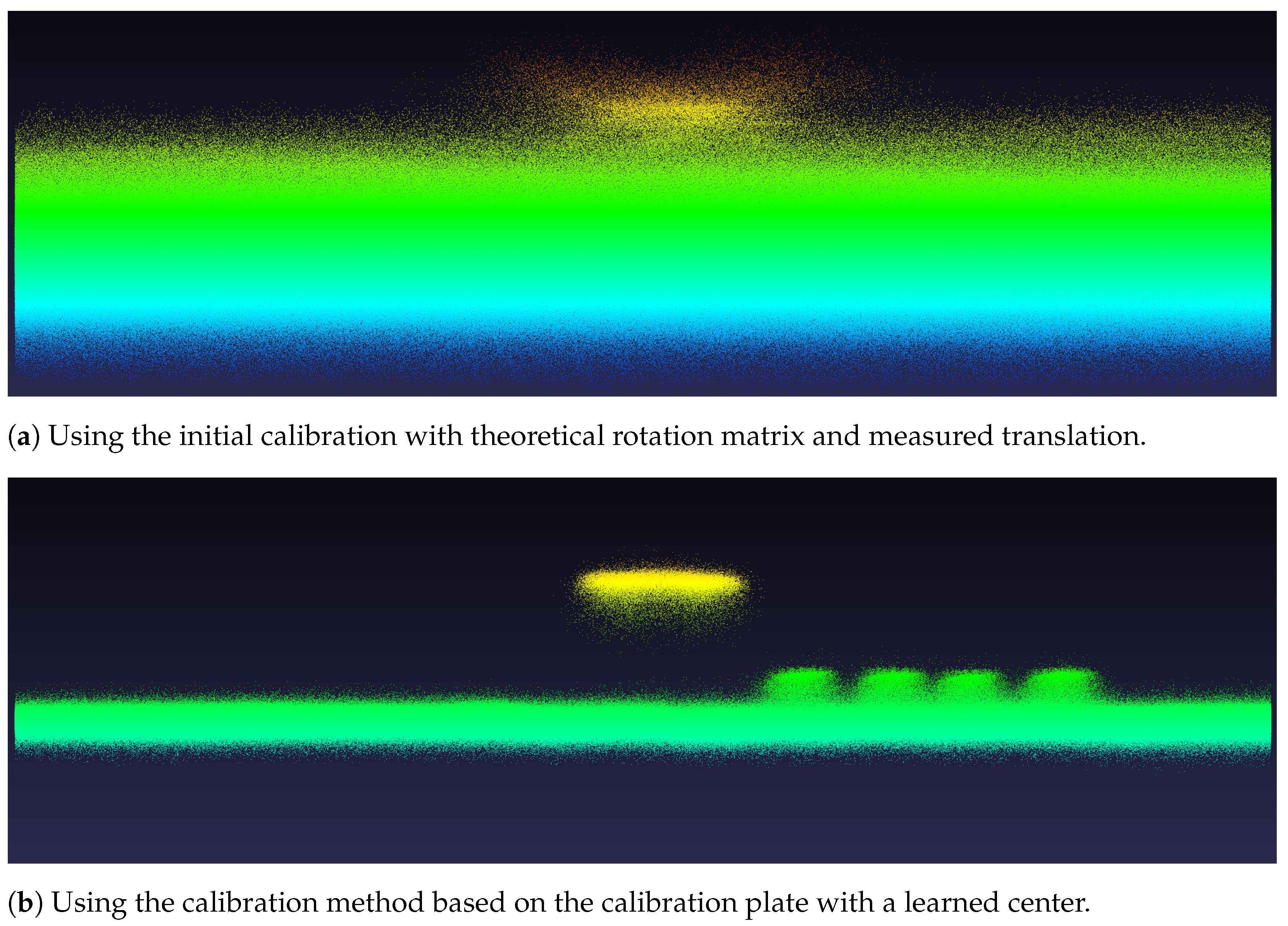
The in-field location was measured using Belgian Lambert 72 coordinates, whereas the Quanta GNSS and hence the LiDAR data use WGS coordinates, which we can easily convert to UTM 31N. Unfortunately, the conversion between Lambert 72 and UTM is not well defined and has only a low accuracy, meaning we cannot actually use this in-field measurement as ground truth. Instead, we also estimated the location of the calibration plate, simply by adding three extra learnable parameters, which we initialized at the converted measured coordinates. Thus, instead of training for consistency with the ground truth, we now trained for internal consistency across all flight lines. We found this approach to work reasonably well, reducing the average error from 1.07 m to 0.186 m. In
Figure 4, we show qualitative results. One can observe that our approach already cleans up most of the calibration noise. Of course, there is still some room for improvement. We plan to employ further consistency measures, such as entropy (for minimization) and consistency in the overlap region between multiple flight lines (i.e., strip adjustment, for maximization). However, this is only important if for the LiDAR registration we would rely solely on the GNSS/IMU data and extrinsic calibration. Instead (see
Section 3.5), we use a dedicated LiDAR point cloud registration algorithm, for which we now have a very good initialization.
3.4. Post-Processing of INS Data
The attitude and position information provided by the Quanta GNSS-aided INS is used to initiate a preliminary alignment of the point clouds captured by the LiDAR scanner. However, GNSS satellite signals are subject to atmospheric effects and to reflection and diffraction caused by interference between radio waves, which in turn leads to multipath errors. To deal with this, the GNSS data are first corrected through post-processed kinematic (PPK), which uses two receivers (one on a nearby base station and one on the Quanta device) instead of one.
Eventually, the raw Quanta data are processed using the Qinertia software from SBG [
20], which applies an extended Kalman Filter (EKF) to couple the GNSS and inertial sensors, allowing the former to correct inertial drift while keeping high frequency (200 Hz) navigation outputs. In
Figure 5, an example of Qinertia’s post-processing is shown. The yellow dots denote the raw GPS point at 1 Hz, whereas the green line denotes the 200 Hz EKF-improved trajectory of the sensor and the drone.
After Qinertia’s post-processing, the standard deviation on the latitude and longitude is about 1 cm. The standard deviation on the altitude is slightly higher and averages around 2.4 cm. While this is reasonably good, minor synchronization errors, time quantization errors (although rather small as the navigation output from the Quanta is 200 Hz), and occasional under-measurements can further affect the accuracy of the resulting point cloud. In addition, the measurements of the Ouster LiDAR scanner have a limited precision of approximately 3 cm for points at a far distance. All this means that the point cloud generated by aligning the scans using the post-processed Quanta data still suffers from significant discrepancies. For that reason, we further improved the alignment by applying a proper point cloud registration technique. As the LiDAR data are particularly challenging (sparse measurements, inhomogeneous point density, etc.) and the circumstances are quite challenging (all points captured from a far distance, few structural elements, and many points sampled on a rather flat ground plane), we developed a novel dedicated point cloud registration algorithm, which is described in detail in the next section.
3.5. Dedicated Point Cloud Registration
Our dedicated point cloud registration consists of two main parts. First, two consecutive point clouds are aligned (scan-to-scan alignment), known in the literature as scan matching. The result is an initial estimate of the relative pose of the sensor. Subsequently, the second point cloud is transformed using the initial estimate combined with the previously computed pose (so-called dead reckoning) to put it in the world coordinate reference system. Then, a second matching is performed between the transformed point cloud and the aggregated point cloud built so far (scan-to-map alignment). The result from the second scan matching increases the accuracy of the final pose estimation since the aggregated point cloud is less sparse compared to the one acquired during one single scan (which often leads to wrong point correspondences). The outline of this point cloud registration work flow is depicted in
Figure 6. Note that, since the aggregation of all point clouds would eventually inflate memory usage, we use a downsampled version derived from an underlying octree data structure.
3.5.1. Scan Matching
The scan matching is computed using a variant of ICP (“Iterative Closest Point”), an algorithm that iteratively determines corresponding point pairs between two point clouds—the source and the target—and uses these to estimate the transformation between the two that maximizes their overlap. Several cost functions to estimate the transformation have been proposed in the literature, such as point-to-point, point-to-plane, and plane-to-plane. The plane-to-plane variant rapidly declines when the scene lacks planar surfaces, which is often the case for outdoor environments such as agricultural fields or vast open areas. The point-to-point cost function lacks overall robustness, making the point-to-plane distance the cost function of choice.
The point-to-plane distance still requires point normals to be calculated for each point in the point cloud. The latter should be performed with care since the accuracy of the estimated pose will largely depend on it. In addition, a proper selection of candidate points is required to achieve a good pose estimation. Points sampled on stable areas, not subject to, for instance, wind (such as the leaves of trees), are preferred as surface normals can be more accurately computed in those regions. Among stable areas are solid surfaces, which are oftentimes planar in the case of constructed environments. In outdoor environments these are less common, but when present (for example facades or rooftops of houses, they should be exploited.
Points that are part of under-sampled or unstructured areas on the other hand should be avoided as they can compromise an accurate pose estimation. However, we should make sure that—at all times—the selected points provide enough
“observability’ of the translation and orientation components along all of the three axes
,
and
. This observability denotes the extent to which the sampled points are able to explain the translation and orientation of the sensor. For example, when the drone is in stable hovering orientation, ground points provide observability of the translation along the
-axis (perpendicular to the ground plane; recall
Figure 2). Facades, in turn, provide observability of the translation along the
- and
-axis (aligned to the ground plane).
We therefore propose two improvements over the original ICP method. First, we proportionate the rotational and translational observability by selecting a proper set of points to make sure that the transformation is not biased towards one particular direction. Second, we incorporate low-level features to add more importance to planar areas. Note that the lack of planar areas in outdoor environments such as agricultural fields does not imply that the scan matching will necessarily fail in those cases. It just will not be able to exploit planarity to increase accuracy.
3.5.2. Proportioning Rotational and Translational Observability
Points sampled on an “empty” flat ground plane will always result in the same pattern in the point cloud, making it impossible to estimate the translation in the directions parallel to the - and -axes. Likewise, if the number of points sampled on the ground plane is too dominant compared to points sampled on objects perpendicular to the ground plane, the standard ICP-based scan matching will fail. Indeed, in that case, ICP will converge to the identity transformation since the way the points on the ground are sampled is the same along consecutive scans. Hence, it is important to select an equal amount of points on structures that are perpendicular to the ground plane; otherwise, ICP will be biased towards the identity transformation (of course, we assume that there are such structures present in the point cloud of a single scan; if not, this would be a degenerate case).
In order to fulfill this constraint, we start by defining the following six “observability” values for each point in the point cloud: , , , . In all these definitions, , , and (in Ouster coordinates), and represents the normal vector of the point . The former three values indicate the contribution of a point to the observability of the three unknown components of the translation vector. The last three values indicate the contribution of a point to the observability of the different unknown angles (pitch, yaw, and roll) of the UAV. Note that points located further away from the sensor contribute more. The idea is to sample points equally distributed among those that score high for each of the six observability values.
3.5.3. Incorporating Low-Level Features
In addition to maximizing the rotational and translational observability, it is also beneficial to select points that are sampled on solid objects such as the facades of houses. One way to deal with this is to scale the observability values from the previous section with an additional value denoting the planarity of the point’s neighborhood, which is defined as , in which , , and are the eigenvalues corresponding to the eigenvectors , , and computed from the covariance matrix of a set of neighboring points of . We thus propose updating the values as follows: , , , , in which denotes the planarity of point . In this way, we give a higher weight to those points that are sampled on “robust” planar regions.
Eventually, we sort the points based on all six values, generating six ordered lists. For every sorted list, we select the N highest-valued points. Note that this implies that fewer than points can be selected in total, as the same point can be part of multiple selected shortlists. The exact value of N is determined through experimental evaluation.
3.6. Stitching of Camera Data
To create georeferenced orthomosaics for the multispectral and thermal image data, we apply structure from motion (SfM) and multiview stereo using the Metashape software from Agisoft [
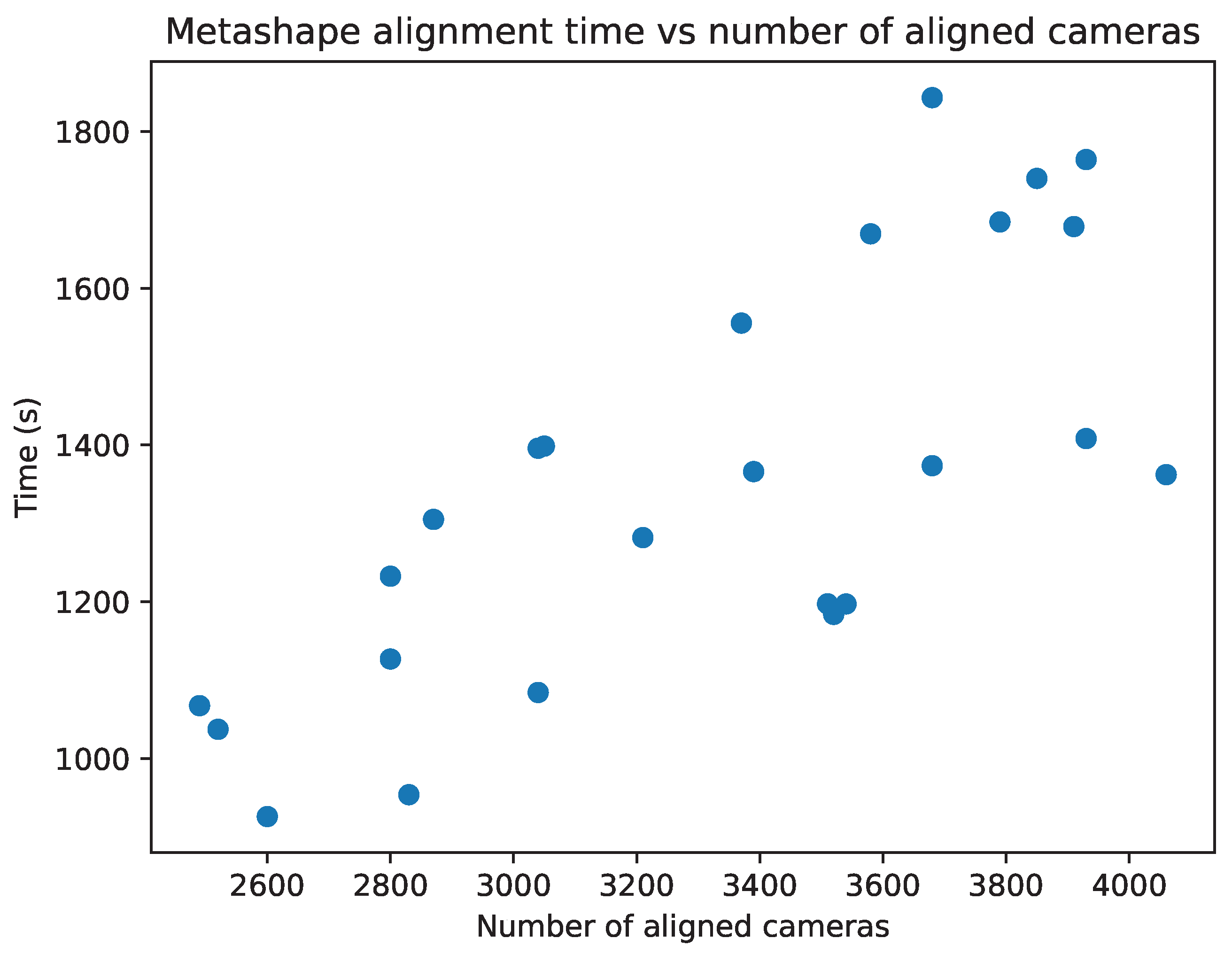
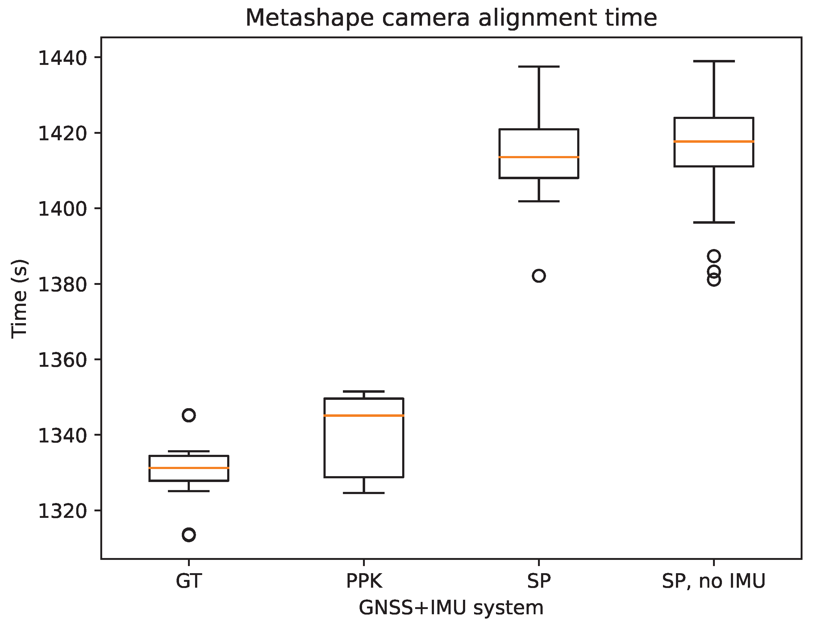
21]. First of all, we calibrate the reflectance via panels we placed in the field and via irradiance sensor data that measure incoming sunlight. We also disable all images obtained while turning the UAV between flight lines or during takeoff and landing. Since all images can be georeferenced with the Quanta GNSS data, this filtering of images is rather easy. Additionally, the GNSS+IMU data, in combination with basic extrinsic calibration between the cameras and the Quanta, allow for a good initialization when aligning the cameras (i.e., computing their poses). After this alignment, we obtain a sparse point cloud, which we filter both using the criteria provided by Agisoft Metashape and by manually removing outliers. Next, we optimize the camera poses and disable those cameras that still have a pixel error greater than 1, followed again by pose optimization.
Given the camera poses, which are now of high quality, we build the dense point cloud, digital elevation model (DEM), and orthomosaic. Using this orthomosaic, we can easily locate our GCP markers in the field and fill in the coordinates we measured on the ground, where we leave the conversion from Belgian Lambert 72 coordinates to Agisoft Metashape. Finally, we optimize the camera alignment again with this new information and rebuild the dense point cloud, DEM, and orthomosaic, which is now properly and fully georeferenced.
3.7. Georeferencing LiDAR Point Cloud and Data Fusion
For the georeferencing of the LiDAR point cloud, we again use the GNSS data from the Quanta (recall that it outputs 200 Hz attitude and position information), albeit in a different way than the image data. For every “firing” of the laser beams, we know the absolute position of the LiDAR sensor (of course after combining it with the Quanta–Ouster calibration), as explained in
Section 3.2, from which we can compute the absolute position of each point. Obviously, since we improved the point cloud registration (and thus the location of the drone), the geolocation of each point was updated accordingly.
To eventually merge the image data from the multispectral and thermal cameras with the LiDAR point cloud, we currently adopt late fusion. The point clouds derived from the structure of the motion process (cfr.
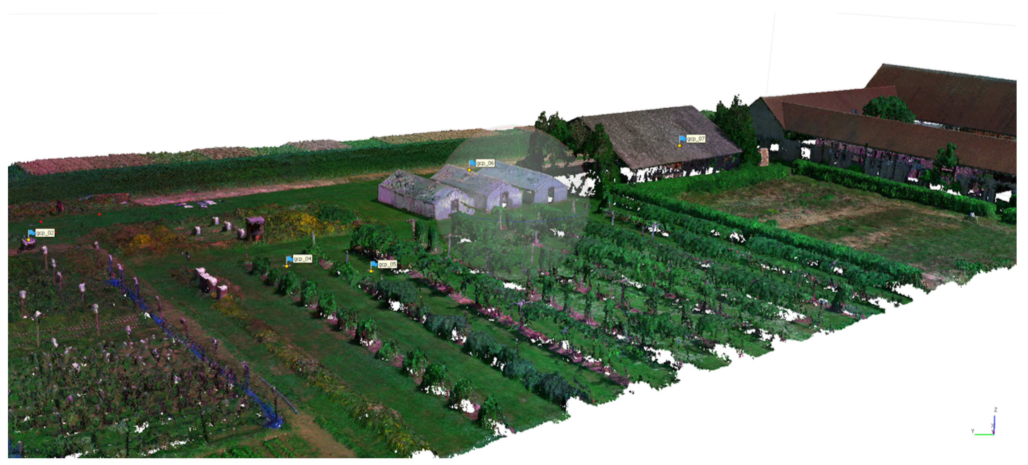
Section 3.6) are inherently aligned with the point cloud generated using LiDAR SLAM through georeferencing. Although we aim for an early fusion approach in the future, late fusion between the multispectral, thermal, and lidar point cloud through georeferencing is quite straightforward. More specifically, we use the accurate (and dense) LiDAR point cloud (or its 2D orthoprojection) as the basis and attribute the spectral information from the multispectral and thermal orthomosaic to each corresponding point. In this manner, we obtain a multispectral point cloud.
5. Conclusions
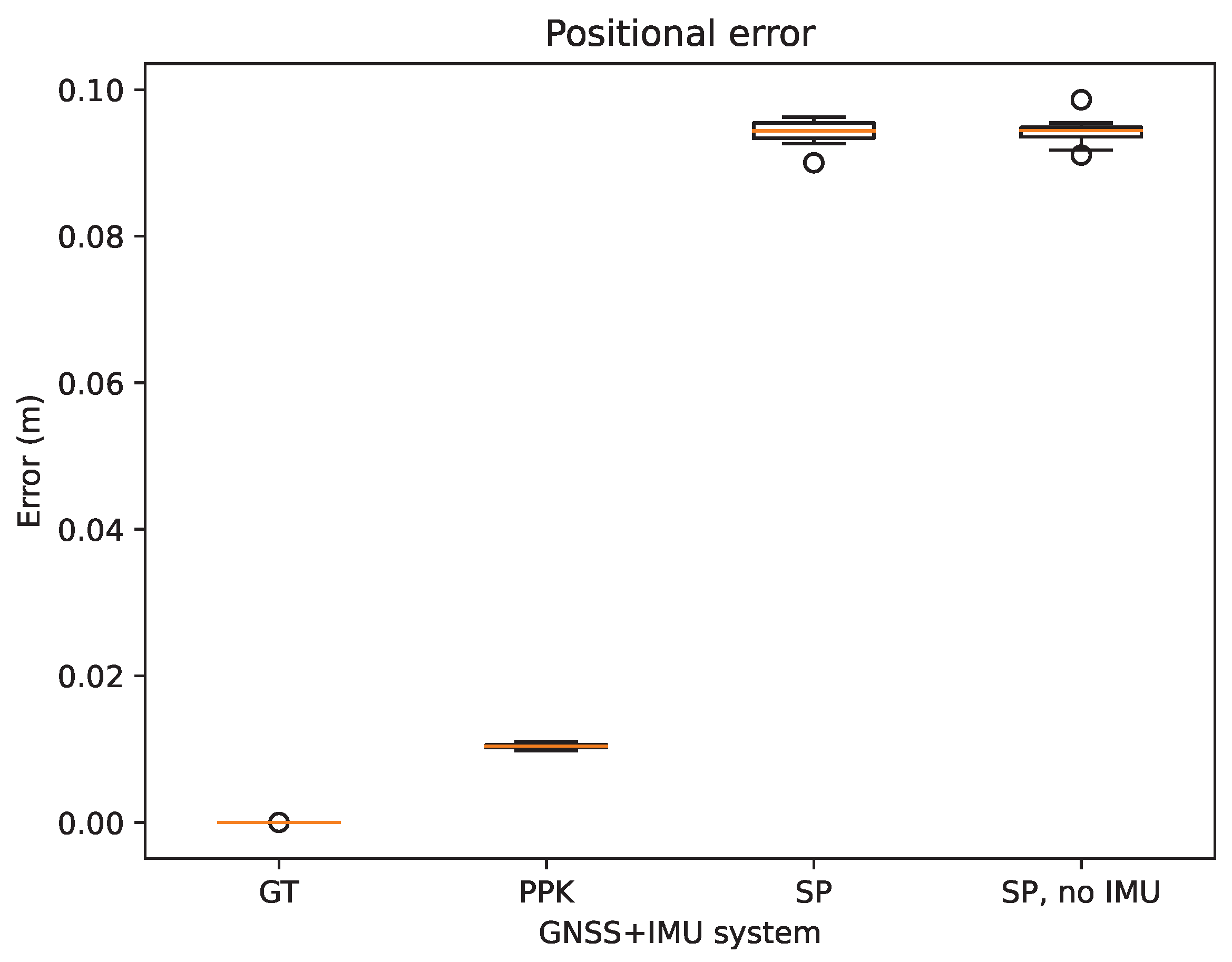
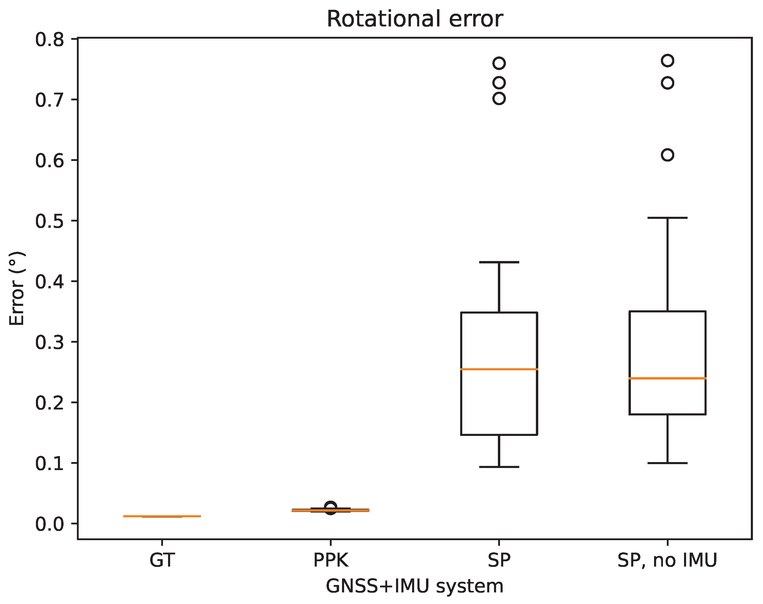
In this paper, we presented our multimodal UAV payload and processing pipeline. The payload consists of an Ouster LiDAR scanner, a Micasense RedEdge dual multispectral camera system, a Teax ThermalCapture 2.0 thermal camera, and a professional-grade GNSS system from SBG. Thanks to the combination of high-frequency navigation outputs from the GNSS and a dedicated point cloud registration algorithm, we obtain highly accurate position and attitude information, which is used to precisely align the data from the different modalities. In addition, for the structure-from-motion process, having access to a high-quality GNSS yields significant improvements, but at least for aerial photography, we found that an IMU is rather optional.
At this moment, late fusion is used to combine the data from the different modalities into one single data structure, being a 14-dimensional point cloud (3 spatial, 1 thermal, and 10 multispectral dimensions) which has subcentimeter accuracy. In the future, we plan to integrate early fusion of the multimodal data in our pipeline in order to more tightly couple the point cloud registration and photometric bundle adjustment, thereby resolving the remaining minor artefacts.

