Article

Method of Infrared Small Moving Target Detection Based on Coarse-to-Fine Structure in Complex Scenes

1
Aerospace Information Research Institute, Chinese Academy of Sciences, Beijing 100094, China
2
Key Laboratory of Technology in Geo-Spatial Information Processing and Application System, Chinese Academy of Sciences, Beijing 100190, China
3
School of Electronic, Electrical and Communication Engineering, University of Chinese Academy of Sciences, Beijing 100049, China
*
Author to whom correspondence should be addressed.
Remote Sens. 2023, 15(6), 1508; https://doi.org/10.3390/rs15061508
Submission received: 6 February 2023 / Revised: 3 March 2023 / Accepted: 6 March 2023 / Published: 9 March 2023

Abstract

:
In the combat system, infrared target detection is an important issue worthy of study. However, due to the small size of the target in the infrared image, the low signal-to-noise ratio of the image and the uncertainty of motion, how to detect the target accurately and quickly is still difficult. Therefore, in this paper, an infrared method of detecting small moving targets based on a coarse-to-fine structure (MCFS) is proposed. The algorithm mainly consists of three modules. The potential target extraction module first smoothes the image through a Laplacian filter and extracts the prior weight of the image by the proposed weighted harmonic method to enhance the target and suppress the background. Then, the local variance feature map and local contrast feature map of the image are calculated through a multiscale three-layer window to obtain the potential target region. Next, a new robust region intensity level (RRIL) algorithm is proposed in the spatial-domain weighting module. Finally, the temporal-domain weighting module is established to enhance the target positions by analyzing the kurtosis features of temporal signals. Experiments are conducted on real infrared datasets. Through scientific analysis, the proposed method can successfully detect the target, at the same time, the ability to suppress the background and the ability to improve the target has reached the maximum, which verifies the effectiveness of the algorithm.

1. Introduction

Infrared imaging has the advantages of strong anti-interference ability, strong concealment, and all-weather work [1]. Due to the development of modern military technology, active radar imaging and visible light imaging cannot meet the actual application. Therefore infrared imaging is widely studied in various fields [2,3,4]. The Society of Photo-Optical Instrumentation Engineers (SPIE) describes a small target as follows [5]:
  • The contrast ratio is less than 15%.
  • The target size is less than 0.15% of the whole image.
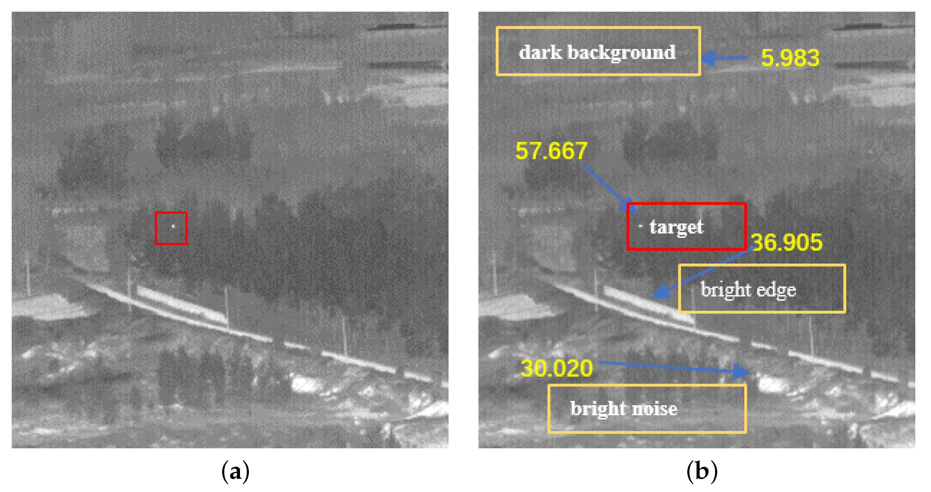
Figure 1 shows two typical infrared images. Targets are marked with red boxes and are shown enlarged. Through the image and the definition above, it can be seen that the target is dim and small. Dim targets mean that the target has a low signal-to-noise ratio (SNR) due to interference from system noise and a large amount of background clutter. Small targets mean that the proportion of the target in the image is very small and the target has no obvious texture features [6]. These characteristics have increased the difficulty of detection. In addition, in the spatial domain, it is difficult to accurately distinguish the target and the noise through the slight difference between the target and the point noise. In the time domain, the target has moving characteristics and the noise is static. This feature can be used to distinguish the target and noise points very well [7]. Although there is a sea of infrared target detection approaches, how to quickly and accurately detect dim and small infrared targets in complex backgrounds, especially for moving targets in the changing backgrounds, the existing methods still face huge challenges [8].
At present, methods based on sequence information and single-frame information are the mainstream approaches in the field of infrared target detection. Methods based on the single-frame information use only limited information from a single image to detect targets [9]. By analyzing the imaging characteristics of the target and the spatial information of the target, a model can be constructed to highlight the target components and suppress the background components [10]. Finally, the results of multiple single frames are formed into a sequence result. This detection method ignores the features in the time domain, resulting in a waste of effective information. However, there is no need to wait for information between frames to accumulate [6]. In the case of high timeliness requirements and general detection effect requirements, more consideration can be given to some of these methods.
Methods based on sequence information use the spatial information of a single image and the temporal information of inter-frame images for detection. This type of detection method comprehensively considers the imaging characteristics of the target and the key information between frames. Multiple information is fused to build a model for target detection [8]. This type of method makes full use of effective information but requires the accumulation of inter-frame information [11].
We proposed an infrared method of detecting small moving targets based on a coarse-to-fine structure (MCFS) in complex scenes. This method makes full use of spatial information and temporal motion features, which has excellent background suppression ability while accurately detecting targets.

1.1. Related Works

The single-frame infrared small target detection methods based on local contrast information have been extensively studied. Extract the information of the target by calculating the contrast feature between the target and the background [12]. Inspired by the human visual system (HVS), Chen et al. [13] constructed a filtering sliding window to obtain the local contrast measure (LCM) of the infrared image to highlight the targets. Wei et al. [14] extracted the target by multiscale patch contrast measure (MPCM) which achieves better performance while some background is still preserved. Moreover, Han et al. [15] used both ratio and difference as computational metrics to calculate the relative local contrast measure (RLCM), which improved detection speed and effectiveness. Chen et al. [16] proposed a small infrared target detection method based on fast adaptive masking and scaling with iterative segmentation by exploiting gradient information to suppress the background components. Furthermore, Han et al. [17] firstly filtered out the low-frequency components of the image and then established a three-layer filter including the target layer, the middle layer, and the outer layer to obtain the three-layer local contrast measurement (TLLCM) of the image, which effectively suppressed the background. Based on the three-layer window, Wu et al. [18] relied on the differences between the three regions to measure the contrast and proposed a double-neighborhood gradient method (DNGM). Lv et al. [19] proposed a computational metric to measure the regional intensity levels (RIL), which received a higher accuracy in the grayscale estimation of infrared images. Inspired by TLLCM and DNGM, and to solve the problem of background clutter, Cui et al. [20] proposed a new RIL (NRIL) weighting function and a weighted three-layer window local contrast measure (WTLLCM) algorithm to further suppress the background residuals. Han et al. [21] proposed an improved RIL (IRIL) calculation method, which solved the problem of noise interference in the traditional RIL and thus proposed the weighted strengthened local contrast measure (WSLCM) to detect the target more accurately. Ma et al. [22] proposed an infrared small target detection approach based on the smoothness measure and thermal diffusion flowmetry through a new thermal diffusion operator. Nasiri and Chehresa [23] proposed an infrared small target enhancement algorithm based on the variance difference (VAR-DIFF) by analyzing the region variances in the three-layer window region. Chen et al. proposed the improved fuzzy C-means clustering for infrared small target detection (IFCM) combined with the idea of multi-feature fusion [24]. Dai and Wu [25] transformed the detection problem into a separation problem by building and solving a tensor model. In order to suppress sparse interference. Guan et al. [10]. introduced the l 112 norm constraint, and added the proposed contrast feature method to propose infrared small target detection via non-convex tensor rank surrogate joint local contrast energy (NTRS). By introducing prior information and calculating the rank, Zhang et al. [26] proposed infrared small target detection based on the partial sum of the tensor nuclear norm (PSTNN). Kong et al. [27] introduced the space-time total variation (TV) norm into the model and used the log operator to approximate the traditional L 0 norm and proposed infrared small target detection via non-convex tensor-fibered nuclear norm rank approximation (LogTFNN). Yang et al. [28] divided the image into different regions and rebuilt the patches to the tensors with the same attributes, and proposed a group image-patch tensor model for infrared small target detection (GIPT).
However, the received images are usually sequential, and only utilizing the information of a single frame image will result in a lack of temporal information. Therefore, many detection algorithms based on multi-frame information have been proposed. Liu et al. [29] proposed small target detection in infrared videos based on a spatio-temporal tensor model by exploiting the local correlation of the background to separate sparse target components and low-rank background components. Du and Hamdulla [30] introduced a spatio-temporal local difference measure (STLDM) method. Zhu et al. [31] proposed an anisotropic spatial-temporal fourth-order diffusion filter (ASTFDF), which first performs background prediction, and then obtains the target image by subtracting it from the original image. Hu et al. [8] proposed the multi-frame spatial-temporal patch-tensor model (MFSTPT) by modifying the construction method of tensors and choosing a more accurate rank approximation. All indicators are greatly improved under the premise of sacrificing a certain amount of time.
In addition, some deep neural networks are also used in infrared dim and small target detection. Hou et al. [32] proposed a robust infrared small target detection network (RISTDnet) combining a deep neural network with hand-extracted features, which successfully and accurately detected the target. Zhao et al. [33] built a five-layer discriminator and added L2 loss to propose a novel pattern for infrared small target detection with a generative adversarial network, which can automatically acquire features. However, due to the imaging particularity of infrared dim and small targets [34] and the lack of datasets [35], the development of deep neural networks is limited to a certain extent. Fang et al. [36] proposed an algorithm for residual image prediction via global and local dilated residual networks (DRUnet). This method proposes a global residual block model and introduces it into U-net [37] with multiscale, leading to successful target detection.

1.2. Motivation

Some existing sequence-based detection methods are effective for detecting targets in simple backgrounds and strong correlations. However, when the background becomes complex and the target varies rapidly, the detection results of either the single-frame-based detection method or the sequence-based detection method are both not ideal. Furthermore, the detection by simple contrast difference can indeed enhance the target, but much clutter, including noise points and bright edges, will be highlighted and falsely detected. Some advanced methods, such as TLLCM, WTTLCM, etc. use Laplacian filtering to smooth the backgrounds which can indeed suppress some background information, but the intensity of the target is also weakened. In this paper, the weighted prior information of the target is combined with the smooth background information to improve the contrast of the target. To solve this problem, multiscale local contrast features (MLCF) and multiscale local variance (MLV) are proposed to extract the potential region of the target (PRT), which can greatly reduce the existence of false alarms while successfully highlighting the target. In addition, the existing calculation method of regional complexity is not accurate enough to estimate the target in the face of dim and small targets in the complex background, resulting in many targets being missed. Thus, a novel robust region intensity level (RRIL) method is proposed. Weighting the spatial features of potential targets by RRIL can more accurately characterize the complexity of the target and suppress the background. Furthermore, in the HVS-based methods [38,39,40], many methods including the sequence-based method do not use the motion information which is very effective in the time domain. Therefore, to employ the temporal information and achieve superior performance, a novel method is proposed for the potential target region by using the motion information of the target. The proposed method is sequence-based detection. Not only the space domain information is used to finely weight the target, but also the time domain kurtosis feature of pixels in different regions is calculated to extract the target and suppress the background. The single-frame image to be detected is in the center of the sequence. Since the information on adjacent frames is needed, we only utilize its spatial information to detect the target at the beginning and end of the sequence, which will reduce the accuracy of some frames and it is also the direction we need to continue to improve. The main contributions of this paper consist of four aspects as follows.
1.
A novel method for extracting coarse potential target regions is proposed. The preprocessed image is obtained by smooth filtering through a Laplacian filter kernel and enhanced with a new prior weight. Next, the multiscale local contrast features (MLCF) and multiscale local variance (MLV) are proposed to compute the contrast difference and obtain the potential region of the target (PRT).
2.
A novel robust region intensity level (RRIL) method is proposed to weight the spatial domain of the PRT at a finer level.
3.
A new time domain weighting approach is proposed through the kurtosis features of the temporal signals to eliminate the false alarms further and finely.
4.
By testing on real datasets as well as qualitative, quantitative, comparative, ablation and noise immunity experiments, the proposed coarse-to-fine structure (MCFS) can achieve superior performance for infrared small moving target detection.
The rest of the article is arranged as follows. The second section introduces the proposed algorithm, including PRT acquisition and weighting in the spatial and temporal domains. The third part demonstrates the experiments and analysis while the fourth and last sections are the discussion and our conclusion.

2. Proposed Algorithm

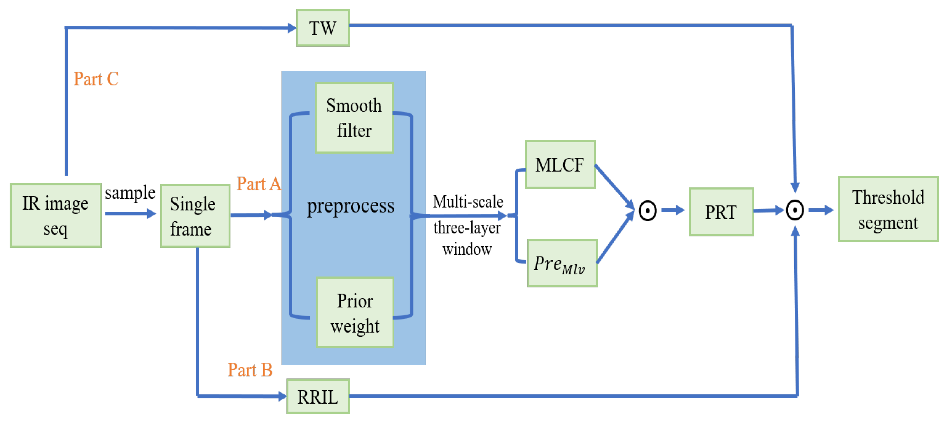
The flow chart of the proposed MCFS is shown in Figure 2. It is mainly composed of three parts: the extraction part of the PRT, the weighted temporal information and the weighted spatial information.
The specific calculation process of the proposed algorithm is as follows:
1.
Firstly, the image is smoothed by Laplacian filtering and combined with the proposed weighted prior weight for image preprocessing, and afterward, the proposed MLCV and MLV incorporating multi-scale strategies are used for local feature calculation to obtain PRT.
2.
Secondly, using the proposed algorithm to calculate a robust region intensity level (RRIL) to obtain the spatial weight of the target.
3.
Then, by using the different moving information of the target and background components, the time domain characteristics of the target are obtained to calculate the temporal weight (TW).
4.
Finally, use the temporal and the spatial weight to finely weigh the PRT and detect the target through threshold segmentation.

2.1. Calculation of PRT

2.1.1. Smoothing Filter

Through the hierarchical model, more contrast features of the target can be obtained to highlight the target and suppress the background. Based on the HVS [38], the brightness of the target is greater than its surrounding background pixels in the infrared image [41], which is due to the local intensity properties [42]. Inspired by Hsieh et al. [43], we build a hierarchical gradient model. It consists of three parts: the target with the larger gray value is located in the center region, and the background with a smaller gray value is located in the outer layer and the transition region, as shown in Figure 3a. Therefore, sliding the layered model as a window in the whole image can obtain contrast information and separate the target from the background.
The energy distribution of the infrared small target is gathered around the center [20]. Therefore, a two-dimensional Gaussian function can be used to simulate a small target [44]. Combined with the idea of a hierarchical gradient model, the Laplacian filter kernel [45,46] is set as shown in Figure 3b. The target information is concentrated in the target layer and the background information is concentrated in the background layer. In general, regions with larger gradient values are more likely to be targeted. In this paper, a common 5∗5 Laplacian kernel is utilized for smoothing and the smoothed image I G is expressed as:
I G ( x , y ) = m = 2 2 n = 2 2 C G ( m , n ) I ( x + m , y + n )
where ( x , y ) is the coordinates of the pixel and C G is the gradient kernel. It can be observed that the weights of the gradient kernels behave as the surrounding energies move toward the center, which can suppress the background components to some extent.
Figure 4a is the original image and Figure 4b is the image after smoothing. The real target is marked with a red box. It can be seen that the background is indeed smoothed.

2.1.2. Weighted Harmonic Prior

Although the Laplacian filter kernel suppresses the background, the intensity of the target is also affected. This means that the background is smoothed, but the contrast of the target is also reduced. To solve this problem, an algorithm to enhance the target is proposed in this paper. Gao et al. [47] pointed out that there are two eigenvalues λ 1 and λ 2 in the structure tensor of each pixel in the image. λ 1 and λ 2 have different relationships when the pixels are at different locations. When λ 1 λ 2 0 , λ 1 λ 2 0 , λ 1 λ 2 0 , the corresponding pixels are located at the flat edge region, the corner region, and the edge region, respectively. The structure tensor is calculated as [47]:
J ρ = K ρ D ρ D ρ = J 11 J 12 J 21 J 22 = K ρ I x 2 K ρ I x I y K ρ I x I y K ρ I y 2
λ 1 = 1 2 J 11 + J 22 + J 22 J 11 2 + 4 J 12 2
λ 2 = 1 2 J 11 + J 22 J 22 J 11 2 + 4 J 12 2
where ∇ represents the gradient calculation, ⊗ represents the kronecker product, I y and I x refer to derivative calculations in both directions, K ρ represents the Laplacian kernel operation, and ρ means the variance.
The edge indicator is more sensitive to the edge information, while the corner indicator tends to highlight the corner information [9]. The parameters of the edge information can be calculated as [26]:
E ( x , y ) = λ 1 λ 2
where E means edge indicator. The parameters of the corner information can be calculated as [48]:
C ( x , y ) = det ( S T R ( x , y ) ) t r ( S T R ( x , y ) ) = λ 1 λ 2 λ 1 + λ 2
where C is the corner indicator, STR is the structure tensor mentioned above, tr is the representation of the trace in the mathematical matrix, and det is the representation of the determinant in the mathematical matrix.
The target is moving and the background is also changing in the image. Only utilizing the edge information to enhance the target may miss the target because the small target is point-like in most cases, and thus the edge indicator does not indicate the structure of the corner. However, it is also unreasonable if we only employ the information of the corners for image enhancement. When the target moves to the edge of the bright background, if only the characteristic of the corners is concerned, the features of the target will be ignored. This can lead to missed targets [49]. Therefore, in the proposed method, we choose the weighted harmonic averaging method for image enhancement as follows:
P I = 1 m 1 C + m 2 E
P = P I min P I max P I min P I
where m 1 and m 2 are the weights of corner information and edge information. PI represents the weight. max P I represents the maximum value in PI, and min P I represents the minimum value in PI. The final normalized weight is P.
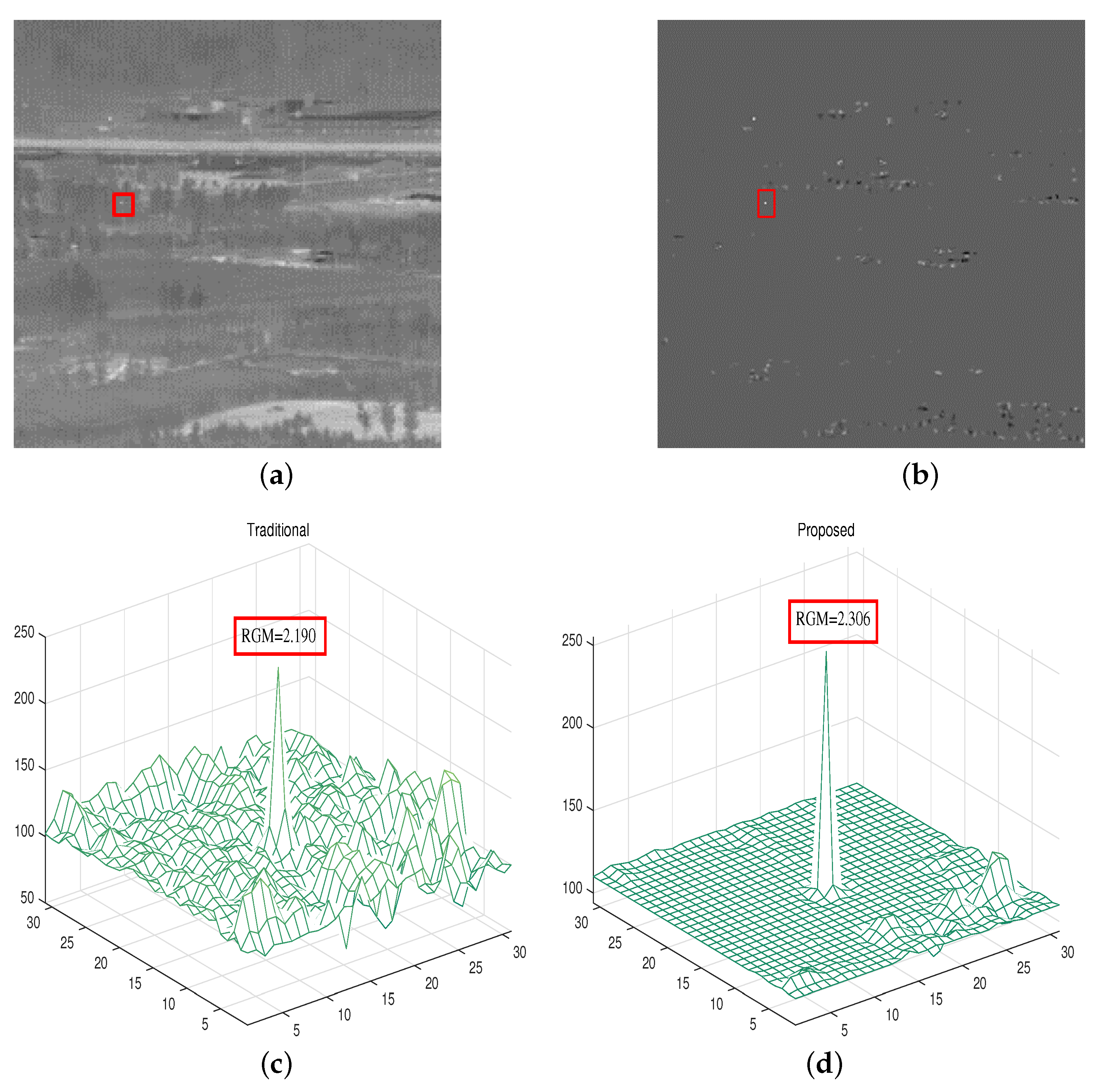
In the experiment, we give large weight to the corner features, which means that we pay more attention to the features of the corners. The image after smooth filtering and weighted prior processing is defined as the preprocessed image, and the calculation of the preprocessed image is shown by
I pre = P I G
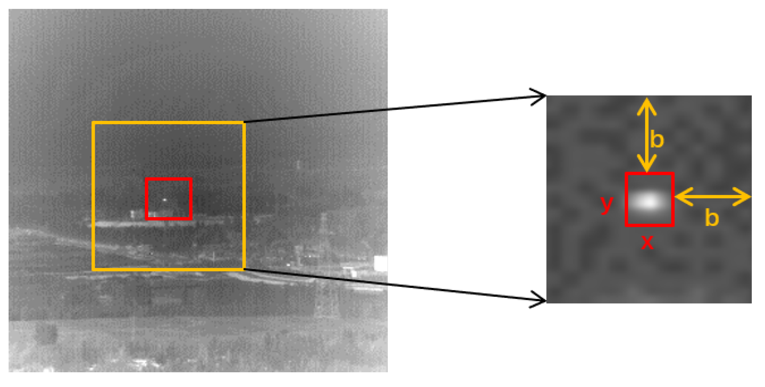
We fix m 2 to 1 and thus when m 1 is less than 1, more attention is paid to the edge information while a heavy weight is assigned to the corner information when m1 is greater than 1. From our previous analysis, we prefer to highlight the features of the corners and set m 1 = 2, m 2 = 1 in this method. Figure 5a shows an infrared image with a complex background, and the real target is marked with a red box. The image is processed by the proposed preprocessing algorithm (Formula (8)), and the result is shown in Figure 5b. The three-dimensional display of the target local region in Figure 4b is shown as Figure 5c, and the three-dimensional display of the target local region in Figure 5b is shown as Figure 5d. Since the comparison of the results of the processed images is not obvious qualitatively, we propose the concept of the ratio of the gray mean (RGM). The meaning of RGM is to calculate the ratio of the gray mean value of the target to the gray mean value of its surrounding local pixels. Here, the size of the surrounding pixels is taken as 25∗25, as shown in Figure 6. From Figure 5 we can see that the RGM of Laplacian filtering merely is 2.190 while our proposed method can achieve 2.306. Therefore, the background is suppressed and the target is enhanced. This proves the effectiveness of the proposed method.

2.1.3. Calculation of MLCF and MLV

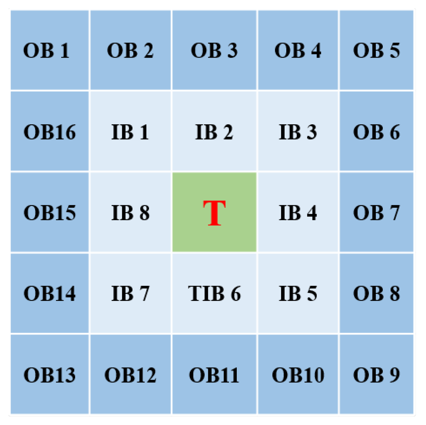
After the preprocessing, the proposed algorithm extracts the PRT in the next step. To detect small targets, Wu et al. [18] designed a filter with a three-layer window as shown in Figure 7. The center window is the region where the target may appear. The outer neighborhood of T has 16 sub-windows and the inner neighborhood of T has 8 sub-windows to compute the contrast differences between the inner and outer neighborhoods. The target is highlighted by the difference in the grayscale shown by.
G ( IB ) = m T max m ( I B i ) , m T > max m ( I B i ) 0 , else
G ( OB ) = m T max m ( O B i ) , m T > max m ( O B i ) 0 , else
L C F = G ( I B ) G ( O B )
where OB is the outer neighborhood. IB refers to the inner neighborhood. m T represents the mean of the target region. m ( I B i ) represents the mean value of the i t h inner neighborhood. m ( O B i ) represents the mean value of the i t h outer neighborhood.
The average value is used to reduce the influence of the highlighted region in the background. However, when facing the corners or edges with strong radiation, the local contrast calculated by that method may also be high, so some background interference is also enhanced, especially for some point interference. The infrared image of Figure 8a is calculated by LCF (Formula (12)), and the result is shown in Figure 9a. The red marks are the target components that we want to highlight. The green marks are false alarm components that we do not want to highlight. It can be seen that some strong interference is also highlighted, which is not the desired result. Through our research, we found that the local variances (LV) of the target and background regions are different. The concept of local variance here is to calculate the variance of each sub-window in Figure 7, including the variance of the target window, the variances of eight windows in the inner neighborhood, and the variances of 16 windows in the outer neighborhood. The variance is calculated as:
L V = 1 n x 1 x ¯ 2 + x 2 x ¯ 2 + x n x ¯ 2
where x 1 x n is the gray value of the pixel in the local region. n is the number of pixels in the local region, and x ¯ is the average gray level in the local region.
We use the LV to acquire the PRT, as shown in Figure 9b, which can be seen that the point noise is suppressed to a certain extent, but some edge clutter is still preserved.

2.1.4. Multiscale Strategy

The size of the small target is generally less than 0.15% of the whole image [5,50]. Although the target is relatively small, the uncertainty of the target size between 2∗2–9∗9 also needs to be considered. For example, for an aircraft target, the entire fuselage can be captured by the infrared probe during the day, but only the engine position can be captured at night, which will cause a small change in the size of the target in the image [51]. Moreover, the movement status of the target may be varied, such as from far to near, from high to bottom and so on. When the target is close to the detector, there are relatively many pixels occupied by the target in the captured image, as shown in Figure 10a. When the target is far away from the sensor, there are relatively few pixels occupied by the target in the captured image, as shown in Figure 10b. To improve the robustness to different target sizes, the sub-window size which is x∗x and determined by the target size, shown in Figure 7, should be flexible and adjustable so that the PRT is extracted by multiscale LCF (MLCF) and multiscale LV (MLV) in this work. Therefore, the final PRT is obtained as:
I P R T = I M L C F I p r e M L V
where I p r e M L V represents the MLV of the preprocessed image. Therefore, we combine the local variance and LCF to calculate the contrast feature of the target. We process Figure 8a through the proposed algorithm (Formula (14)), and the result is shown in Figure 9c. The results illustrate that the target has been enhanced, and the background components have been greatly suppressed, which proves the effectiveness of the proposed method.

2.2. Calculation of Spatial Weighting Map

After the PRT is obtained in the first section coarsely, a finer extraction is required to obtain a more accurate position of the target. The RIL [19] improves the accuracy, but is easily affected by high-intensity noise. In other words, the existing calculation methods are not robust, and the evaluation is inaccurate when the target is located in a uniform background. When the target moves to the edge of the high radiation region or there is a bright background region around the target, the evaluation effect needs to be improved. Therefore, a robust RIL (RRIL) calculation method is proposed in this paper. R R I L i is calculated as:
A R R I L i = M k ( i ) min ( m e a n ( i ) , m e d i a n ( i ) )
B R R I L i = M k ( i ) M k m i n ( i )
R R I L i = A R R I L i B R R I L i
where M k ( i ) , m e a n ( i ) , m e d i a n ( i ) , M k m i n ( i ) represent the mean value of the top k largest pixels, the mean value of the pixels, the median value of the pixels, and the mean value of the last k smallest pixels in the i t h region in Figure 7, respectively. ARRIL and BRRIL calculate the RRIL at the same time to ensure that the target region always has a larger response value.
The positional relationship between the target and the background can be roughly divided into four cases in Figure 11. The gray value of the small target in the infrared image may not be the largest in the whole image, but it is generally larger than its surrounding local area [18]. The numbers, for example, in the figure are grayscale values. The green cell is the target, represented by the grayscale values of 255. The blue cell is the bright background, represented by the grayscale value of 210 and the gray cell is the dark background, represented by the grayscale value of 10.
1.
In most cases, the relationship between the target and the background in infrared images is shown in (a). The target is bright, and all the surrounding background areas are dark. At this time, the response of the target processed by either ARRIL or BRRIL calculation is large. So the multiplied response must also be large.
2.
There is sparse point-like bright noise around the target, as shown in (b). The response of the target calculated by BRRIL is large. Due to the existence of the median value in ARRIL, the calculated response is also large. So the multiplied response is also large.
3.
There are multiple point noises around the target or the target is at the edge of the bright background region, as shown in (c). At this time, although the response obtained by the target through ARRIL is small, the response obtained by BRRIL is large. So the response of the final target is large.
4.
The target is in the highlighted background region, as shown in (d). Although both ARRIL and BRRIL will be small, the background response is smaller. At the same time, this situation will be suppressed during the extraction of PRT.
Finally, the spatial weighting map is computed as:
R R I L = max ( R R I L T mean R R I L T O B i , R R I L T mean R R I L T I B i ) I L V
where R R I L T is the RRIL of the target area. R R I L O B i , and R R I L I B i are the RRIL calculated by the i t h area of the outer and inner neighborhoods, respectively. I L V represents the local variance of the original images. The purpose of using the mean is also to improve robustness.

2.3. Calculation of Temporal Weighting Map

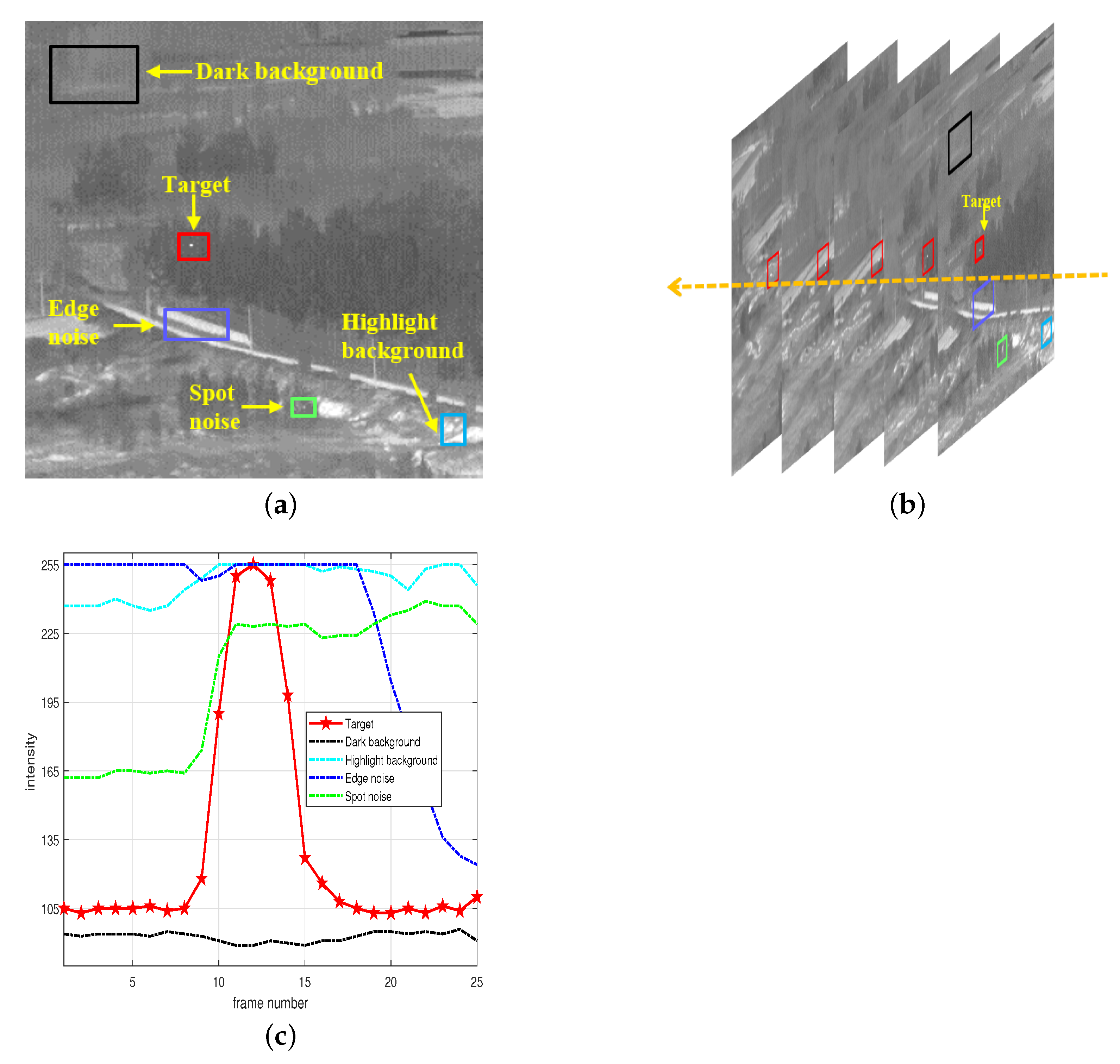
After coarsely obtaining the PRT, the time domain weighting is required to suppress more clutter and increase the detection accuracy at a finer level. In infrared images, targets are generally brighter than the surrounding background [17]. When the infrared small moving target passes through a certain position, the gray level of this position will vary from dark to bright and then from bright to dark. Figure 12a is a typical infrared image with multiple types of local regions which are marked with boxes in different colors. The cumulative change of the pixels at each position over time is recorded. Figure 12b shows the gray intensity change curve of each region in the time domain. The time-domain intensity distribution curve formed by the target movement is similar to Gaussian [7] distribution. In probability theory and statistics, kurtosis is a measure of the “tailedness” of the probability distribution of a real-valued random variable. The kurtosis can describe the steepness and gentleness of the distribution [52]. A normal distribution has a kurtosis of 3.
The variation characteristics of pixels in different regions are reflected in different magnitudes of kurtosis. Therefore, different positions can be weighted by calculating the kurtosis features of the time-domain signals formed by the pixel values of the infrared sequence images. The kurtosis of a distribution is defined as:
k = E X μ σ 4
where μ is the mean, σ is the standard deviation, and E is the expectation operation.
The part C in Figure 2 is to finely weight the coarse target through the temporal weight. The temporal weighting (TW) map can be calculated as:
T W = k u r t o s i s ( I s e q )
where I s e q is the pixel gray value in the input image sequence. Coarse targets are finely weighted by spatial and temporal information.

2.4. Calculation of Target Feature Map

Combining the information in the spatial and temporal domains, the target feature map T of the target is finally formed as:
T = I P R T R R I L T W
Finally, the position of the target is obtained through the adaptive threshold as:
m + v v a r
where m and var are the mean and the variance of the target feature map, respectively, and v is an adjustable parameter to determine how much to weight the variance in the threshold segmentation.

3. Experiment and Analysis

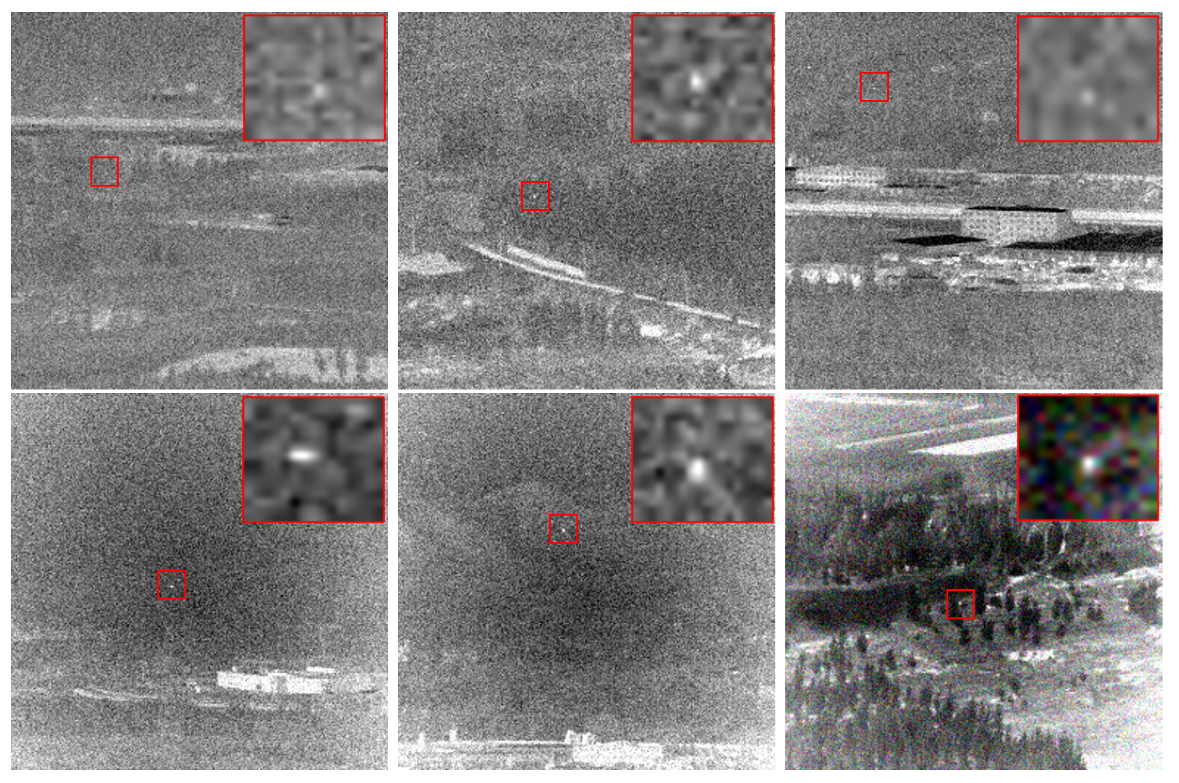
In this section, we tested six real infrared sequences, and nine state-of-the-art methods are employed for comparisons.

3.1. Dataset Introduction

This data set is used in low-altitude aircraft target detection and tracking [53]. The data information is shown in Table 1.

3.2. Parametric Analysis

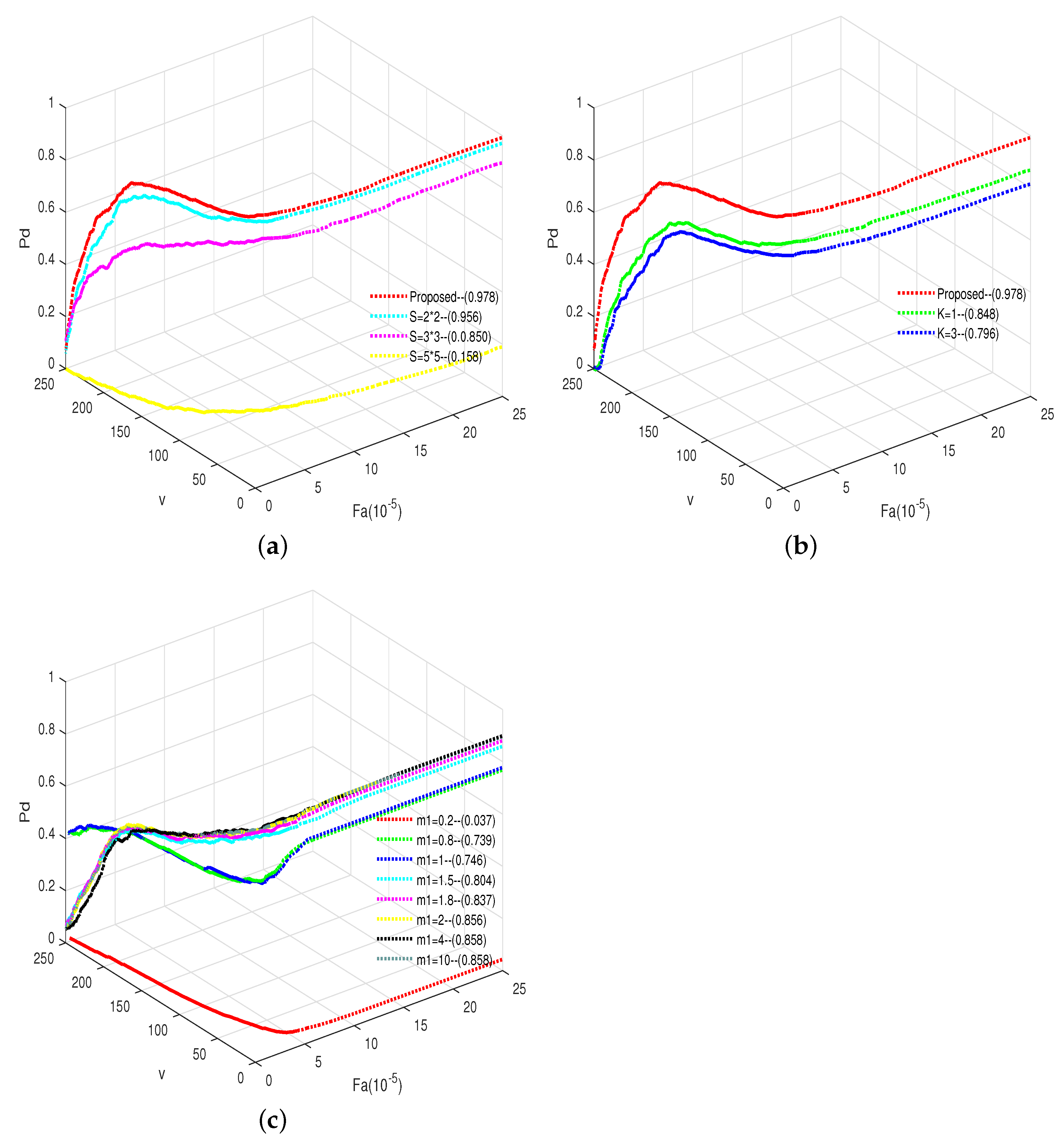
To obtain accurate parameters, we performed a parametric analysis. It mainly includes the setting of parameters in multiscale, the size of K in RRIL and the size of the assigned weight in the prior weight. Since the size of the target in this dataset is no larger than 3∗3, the multiscale parameters are set to 2∗2, 3∗3 and 5∗5 for analysis. The comparison performance is shown in Figure 13a. Since the smallest scale parameter is 2∗2, the size of K must be less than 4. Thus, K was set to 1, 2 and 3 in the analytical experiments and the results are shown in Figure 13b. In the experiment, m2 is fixed to 1. Different weights are obtained by changing the size of m1 and the obtained results are shown in Figure 13c. Numbers in the legends show the area under the curve (AUC) [54].
It can be seen that setting the size of the window to 2∗2 or 3∗3 alone gives much better results than 5∗5. This is determined by the size of the target in the image. However, as mentioned above, setting the window to a fixed size has certain drawbacks. The proposed method sets the window to 2∗2 and 3∗3 with multiscale strategies, which is added to Figure 13a–c. It can be seen that the obtained results are indeed improved, which verifies the effectiveness of the method. Moreover, the weight obtained by the spatial weighting is greatly affected by K. Since K is less than 4, it can be seen from the results that the AUC obtained by setting K to 2 is the highest. Different m 1 and m 2 mean different specific gravities. In addition, when m1 is less than 1, more attention is given to the edge and the AUC is relatively small, which is in line with the theoretical analysis. When m 1 is greater than 2, such as m 1 = 4 and m 1 = 10, the results are no longer significantly improved. So we set m1 to 2 in this method.

3.3. Ablation Experiments

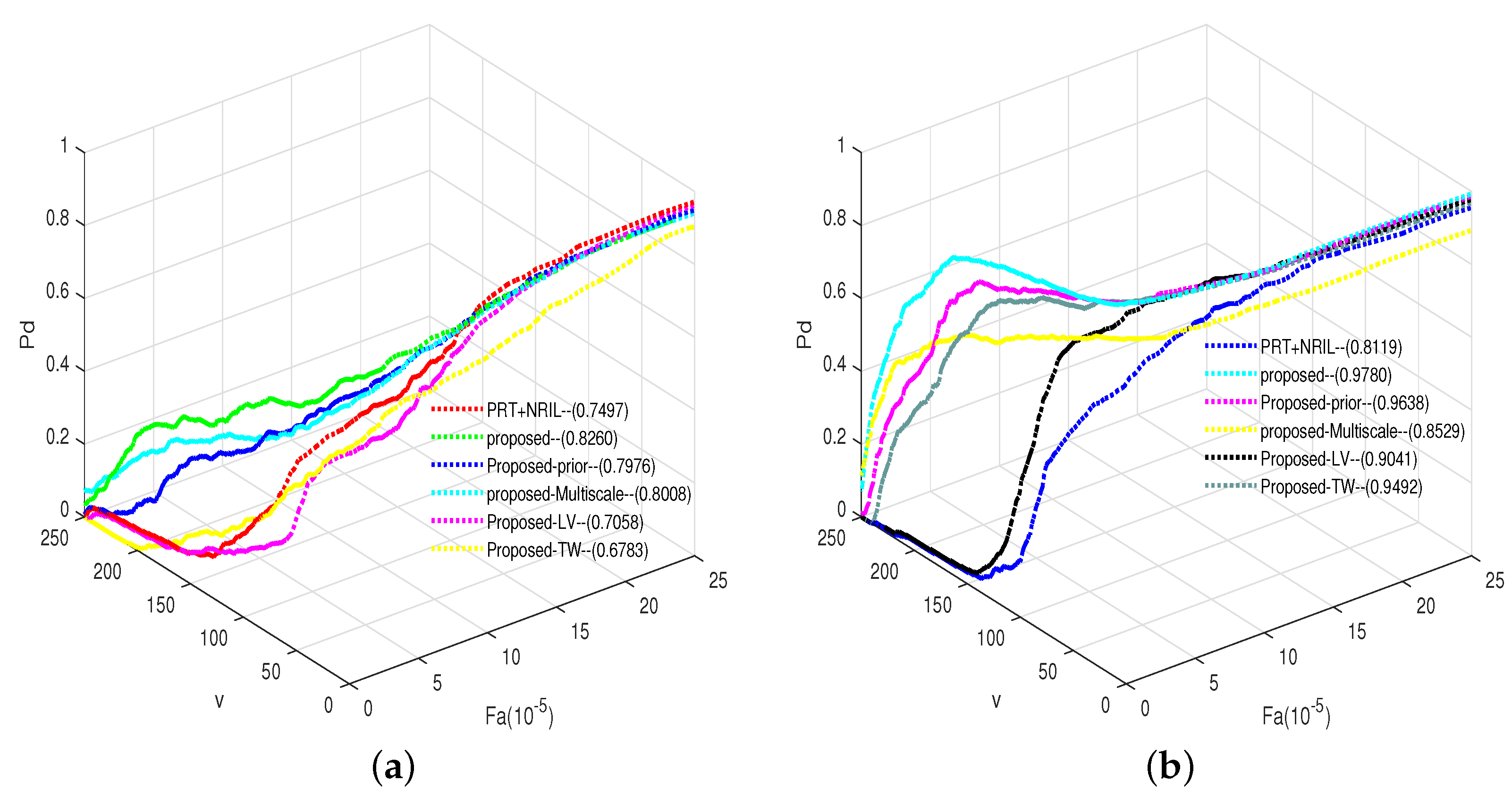
To verify the effectiveness of each part, we performed the ablation experiment as shown in Figure 14. Ablation experiments were performed separately in two sequences. The “-” in the legend is the experiment performed by removing a certain part of the proposed algorithm.
It can be seen from the results of the ablation experiments in Figure 14 that the performance of the proposed complete algorithm is superior to removing or replacing any one module, which proved that each part can improve the detection performance.

3.4. Qualitative Analysis

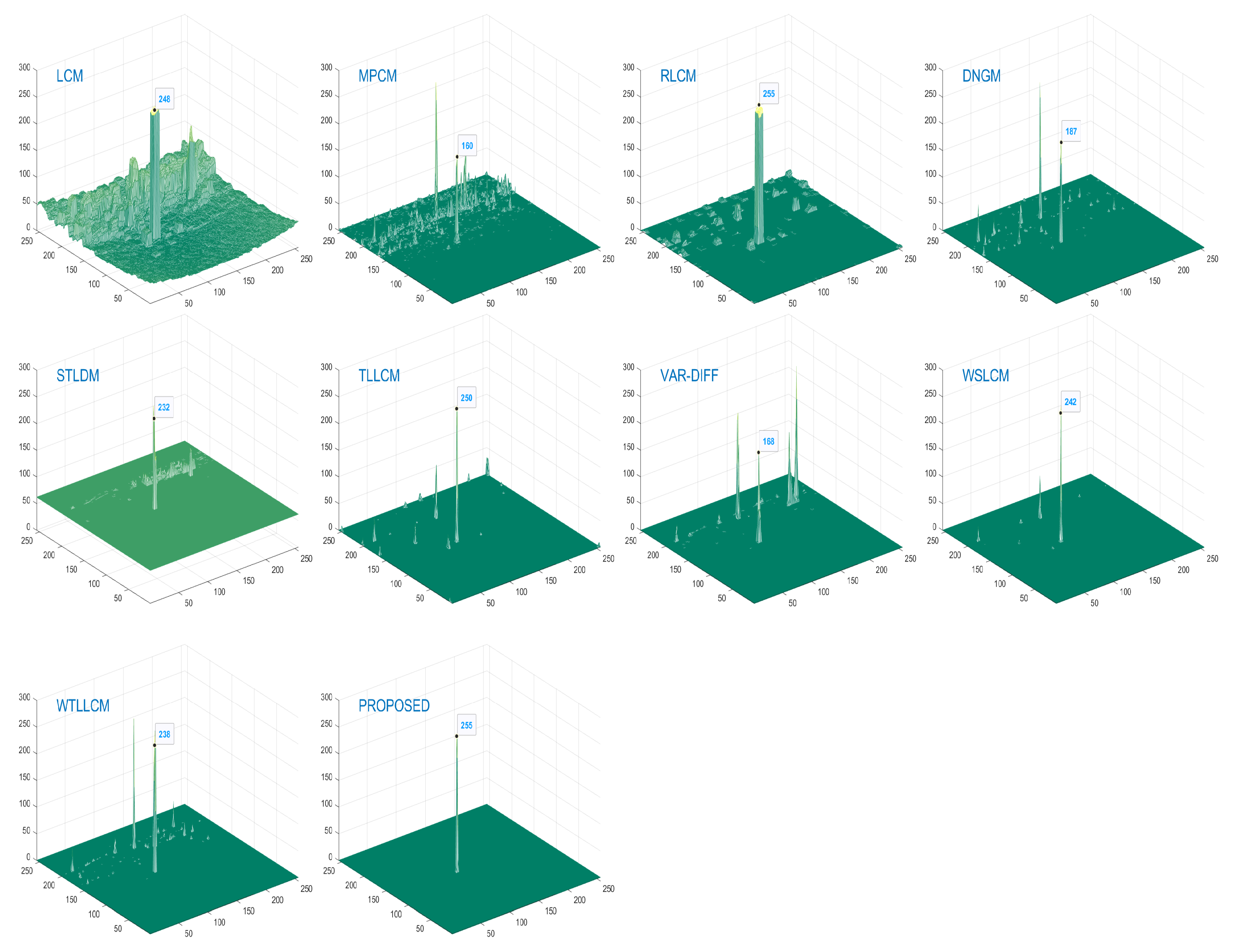
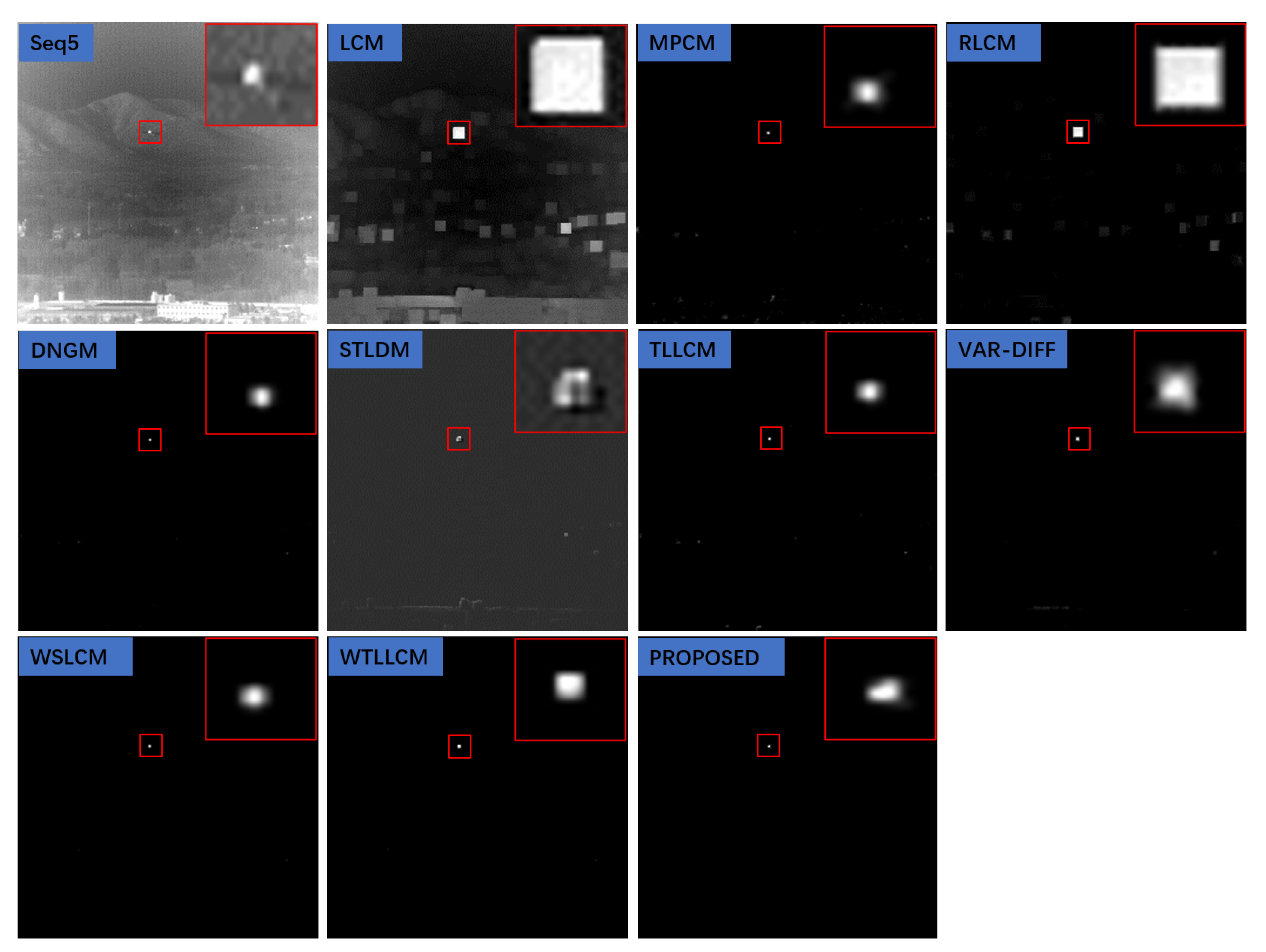
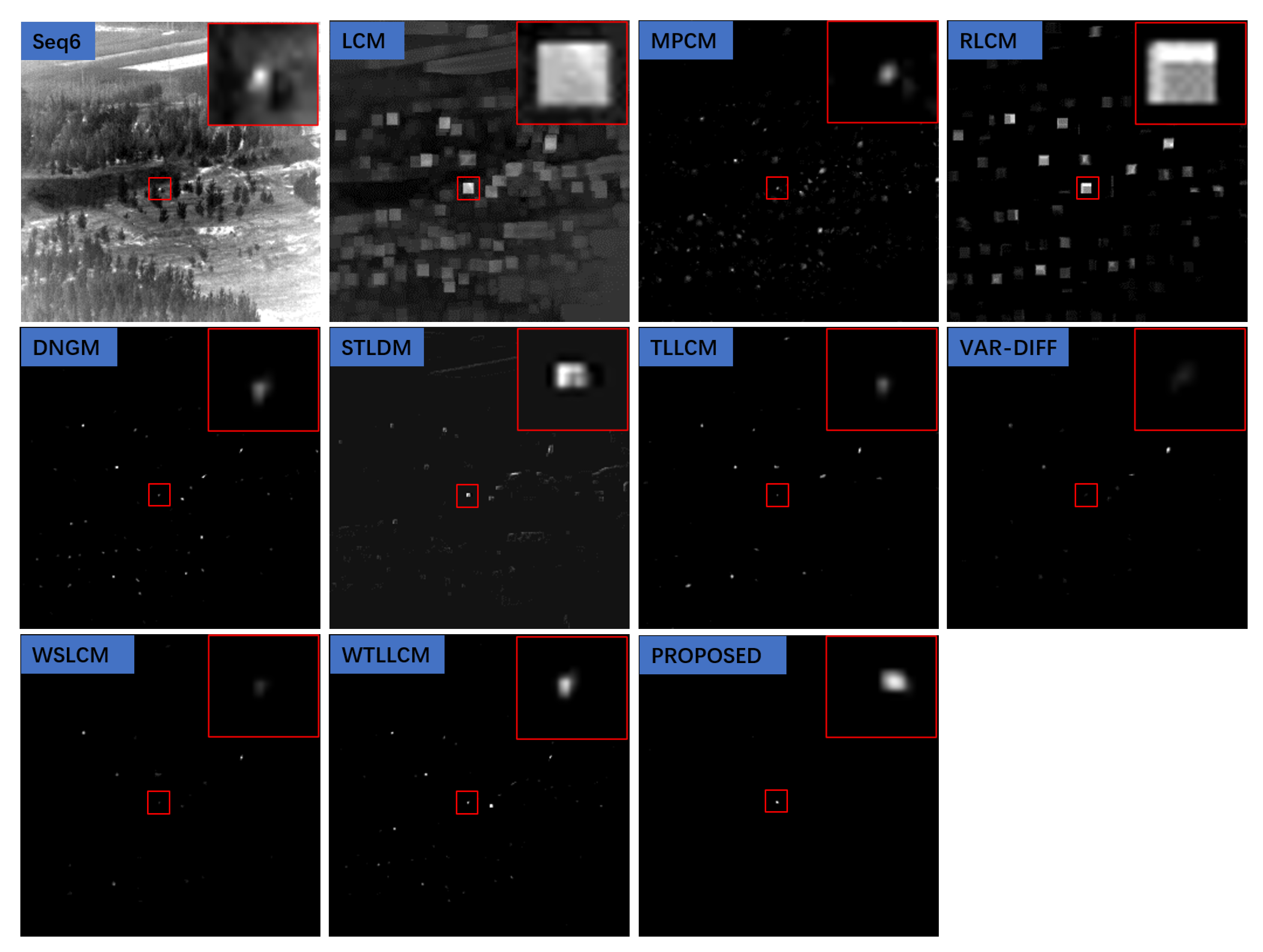
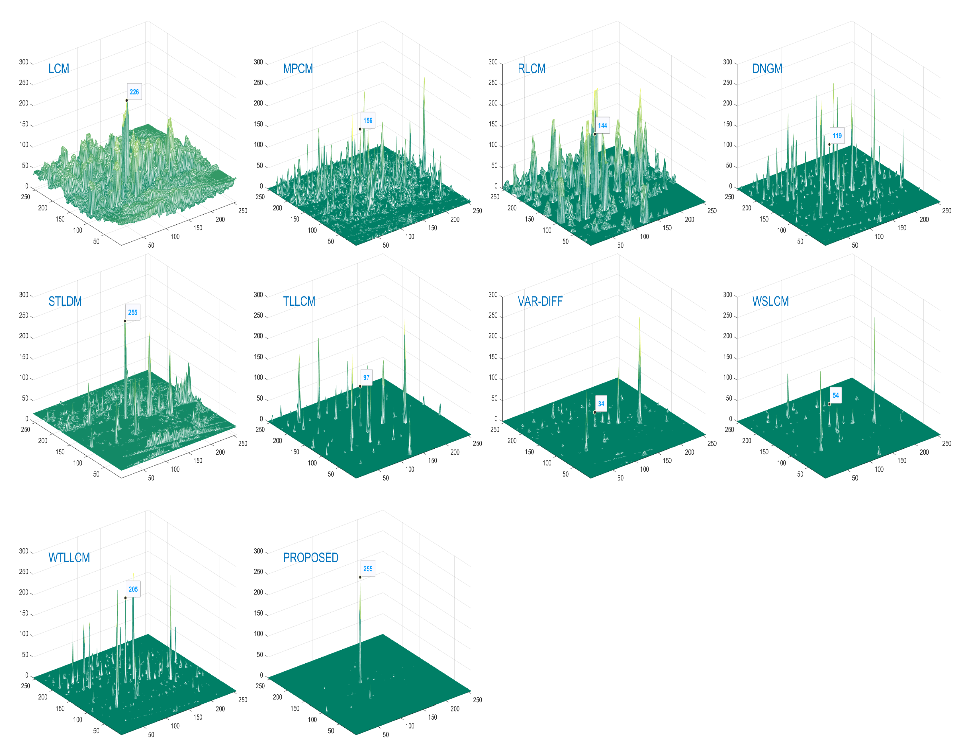
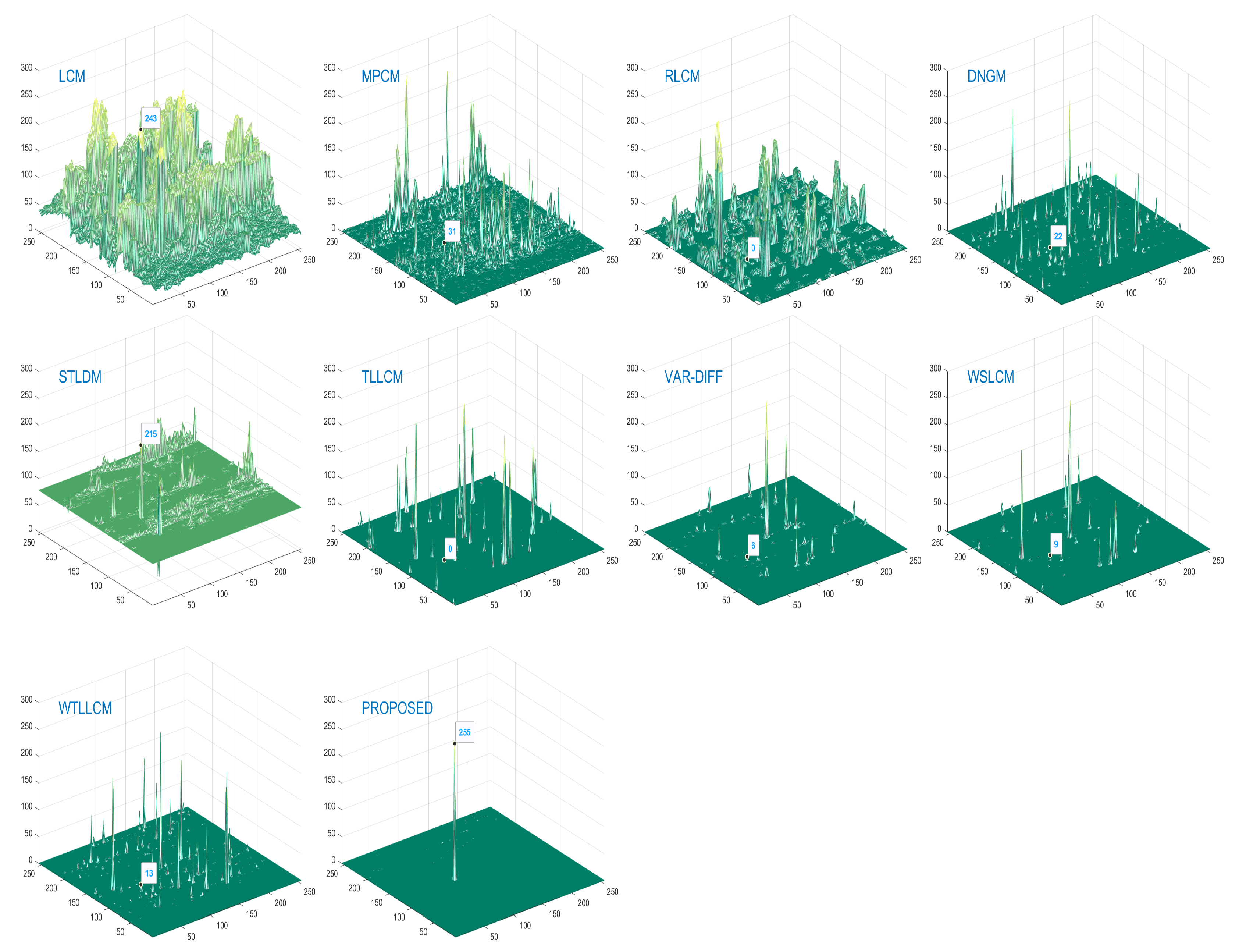
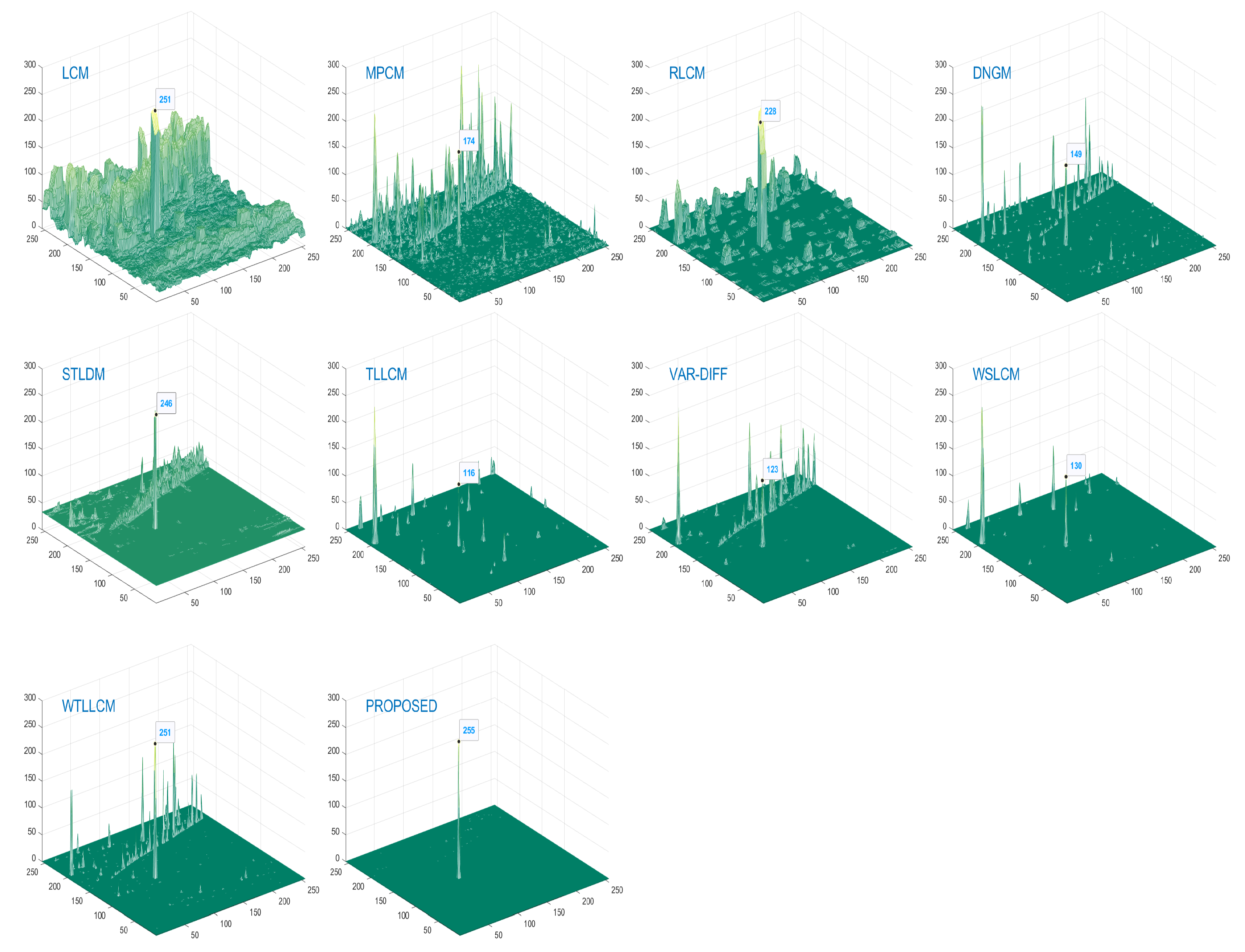
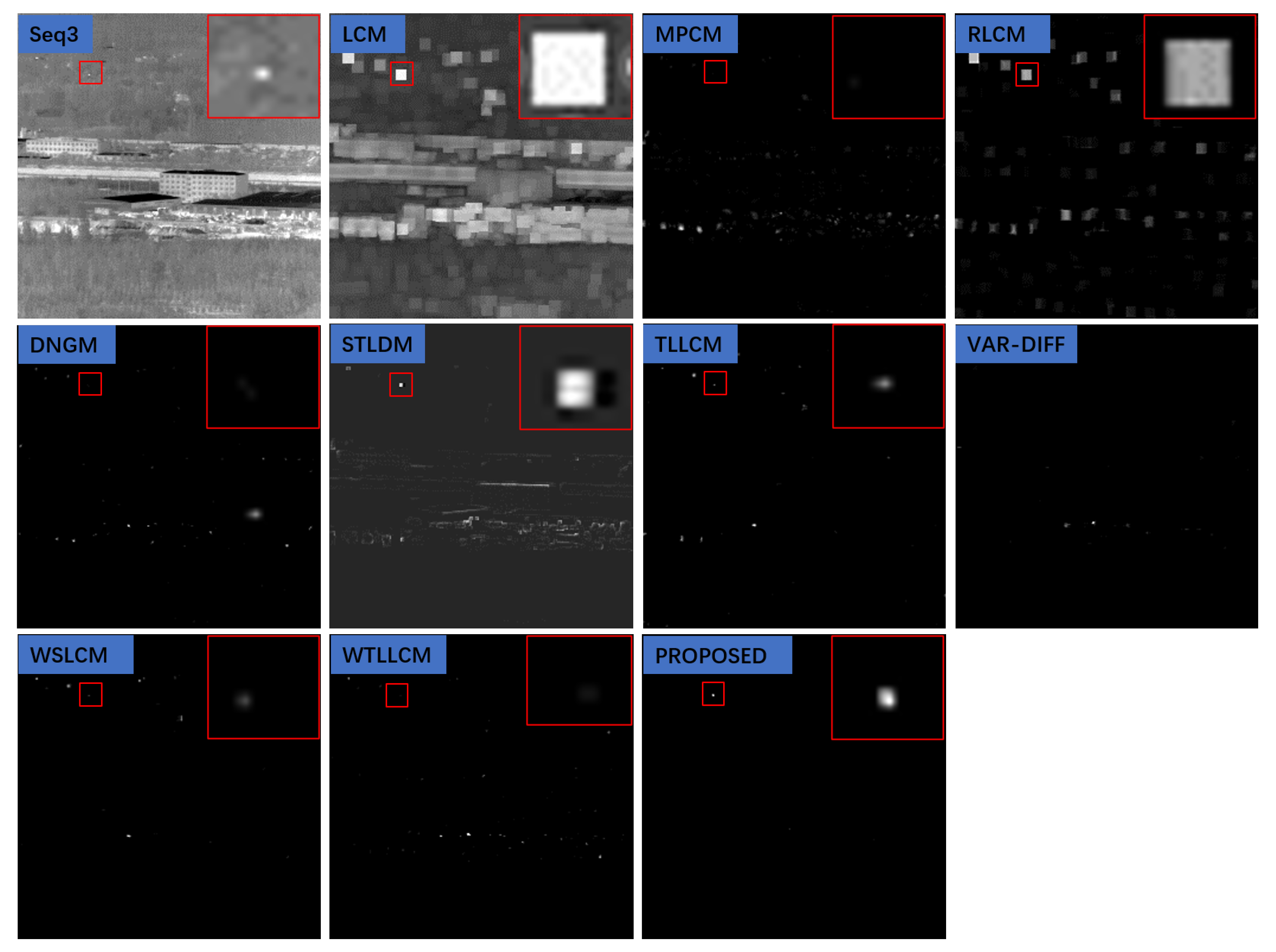
To illustrate the superiority of the proposed method, we ran the nine references and our proposed method on each of the six datasets, mainly including the typical HVS-based methods and some novel HVS-based approaches whose experimental parameters are listed in Table 2. We show the results of datasets 1 to 3 in Figure 15, Figure 16, Figure 17, Figure 18, Figure 19 and Figure 20 and other results on datasets 4–6 are shown in the appendix. The figures contain images of the detection results of each algorithm in the three datasets and the three-dimensional display of the detection results. The rest of the experimental results are in the appendix. The first image in each set of results is the original infrared image, and the rest are the detection results of each method. Each red box in the detection result is the target position manually marked according to the label. The other highlighted parts except the red box are false alarm components that we do not want to highlight. The position of the number in the three-dimensional display is the position of the target and the size of the number is the obtained target response. The other parts except the numbers are the false alarm components that we do not want to highlight. For better observation, we zoomed in on the target and placed it in the corner of the image. Unmarked is the case of missed detection. In addition, all of the experiments were implemented with Matlab in Windows 10 based on Intel(R) Core(TM) i5-8250U 1.60 GHz CPU with 12 G of RAM of a desktop computer.
It can be seen from the results that LCM enhances the target while the background is enhanced as well. The detection effect of MPCM in a complex background is very poor, and there are a large number of false alarms. RLCM does highlight the target, but as in data6 and data1, many noise disturbances are also enhanced. There are cases where the background is not zero in STLDM. Furthermore, STLDM is sensitive to edge noise, which is not an ideal result. The detection ability of TLLCM and WTLLCM is worthy of recognition when the background is simple, such as data4 and data5. However, the information of clutter cannot be suppressed in the complex background, such as data2 and data6. WSLCM has a lot of false detection information in the complex background, such as Figure 16, Figure 20 and Figure A6. Moreover, the target response obtained is relatively small, which needs to be improved. There are edge-like false alarms in VAR-DIFF. However, our proposed method accurately detects the target with the fewest false alarms. In addition, it can be seen from the three-dimensional displays that the proposed method has the largest target response and the largest ability to suppress the background, which proves the superiority of the proposed method.

3.5. Quantitative Analysis

3.5.1. Evaluation Indicators

In this experiment, several typical evaluation indicators were selected for qualitative analysis, including:
  • Background suppression factor (BSF) [55]:
    B S F = δ i n δ out
    BSF is a measure of the ability of the algorithm to suppress the whole background. δ o u t represents the standard deviation of the whole background region of the processed image. δ i n represents the standard deviation of the whole background region of the input image.
  • Signal-to-clutter ratio gain (SCRG):
    S C R = μ t μ b σ b
    S C R G = S C R out S C R in
    SCRG is an indicator used to measure the ability of the algorithm to improve the local contrast of the target. μ t represents the gray mean of the target. μ b and σ b represent the gray mean and the variance of the local background region around the target as shown in Figure 6. In this experiment, we take b as 25. S C R o u t and S C R i n represent the processed image and the SCR of the input image, respectively.
  • Area under the curve (AUC). AUC is related to detection probability ( P d ) and false alarm rate ( F a ):
P d = O T A T F a = F P T P
Among them, OT represents the number of targets in the output image and AT represents the number of targets that actually exist in the sequence. FP represents the number of pixels in the false alarm area and TP represents the total number of pixels in the image sequence. The receiver operating characteristic (ROC) curve can be drawn from P d and F a , and the area under the curve (AUC) can be calculated. It is worth mentioning that the larger the SCRG, BSF, and AUC, the better performance of the method is.

3.5.2. Quantitative Evaluation

In order to measure the performance of each algorithm more accurately, the detection results are quantitatively analyzed. The obtained results are shown in Table 3 and Table 4.
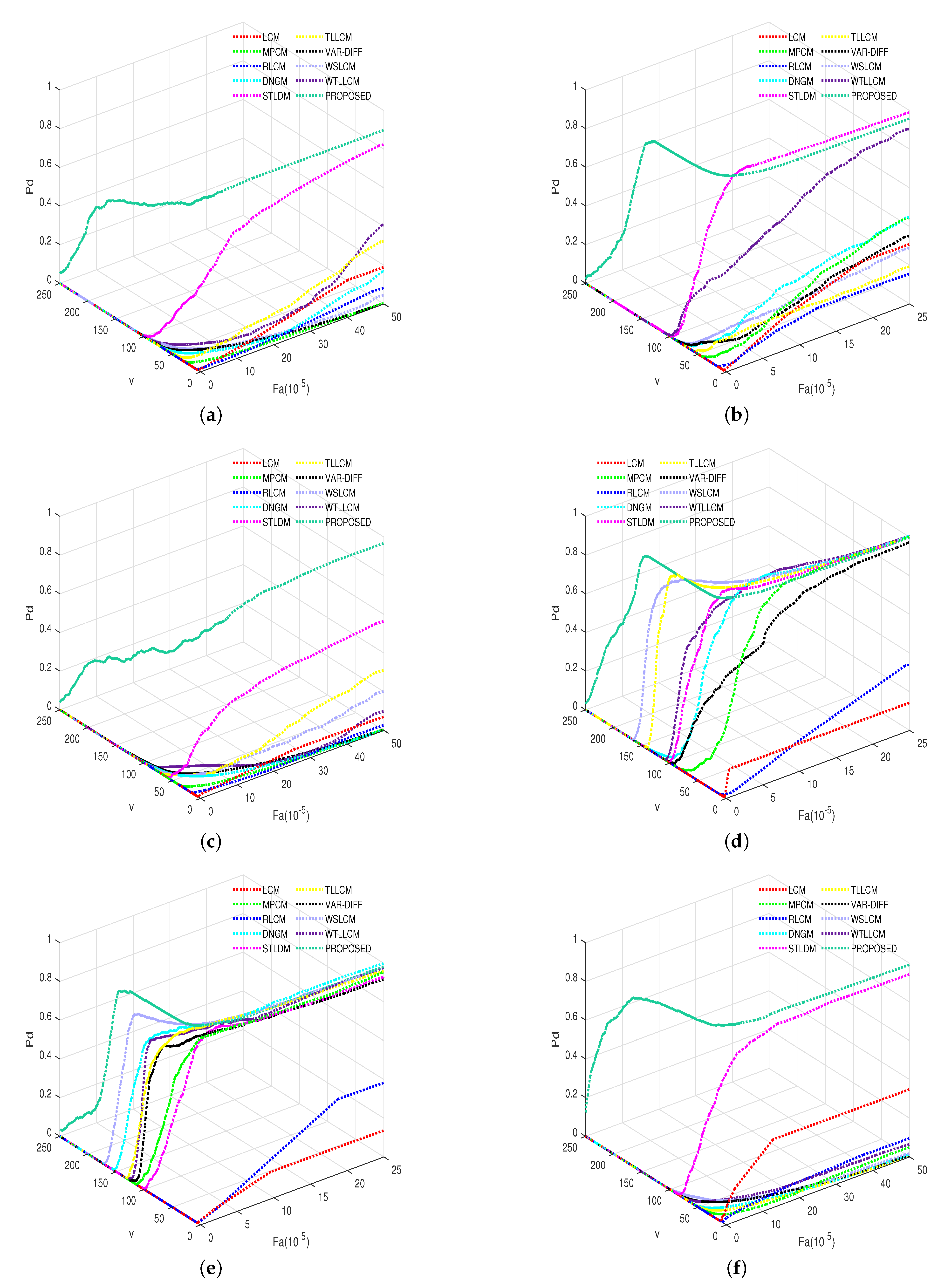
The larger the evaluation indicators in the table, the better performance the algorithm achieves. For each metric, the best results are marked in red. V in the 3-D ROC curves is the parameter mentioned in Equation (22). As shown in Equation (22), in a target map, its mean value and variance are determined. So we obtain different thresholds by setting different v. Furthermore, each obtained threshold will obtain a set of P d and F a . By setting multiple v, multiple thresholds can be obtained to further obtain multiple P d and F a . Therefore, the ROC curves can be plotted. The ROC curves of each algorithm in 6 sequences are shown in Figure 21.
It can be clearly seen that the proposed method has achieved very significant advantages in terms of BSF, which proves that the proposed method has the strongest ability to suppress the background. Except for the AUC in data3, the AUCs of the proposed method all reached the maximum value in the remaining five sequences. This proves that we accurately detect the target while the probability of false detection is minimized. For SCRG, although the proposed method does not reach the maximum in some data, it also achieves very competitive results. In conclusion, it can be demonstrated by the tables and figures that the proposed method achieves superior performance.
Furthermore, it can be seen from the ROC curves and the corresponding AUC values that the proposed method achieves the best performance. LCM, MPCM, and RLCM have poor detection performance in complex backgrounds because they simply use contrast differences for detection, which will cause many false detections. STLDM and TLLCM have poor anti-interference and the results have large fluctuations, which is not a robust result. Through data analysis, it can be concluded that the proposed method achieves the best results in false alarm rate and accuracy rate.

3.6. Robustness to Noise

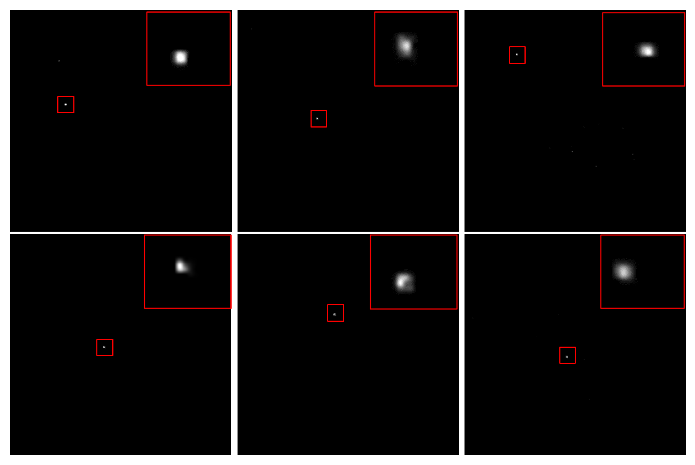
In the infrared imaging system, there will be a certain amount of noise in the environment or the instrument itself. Therefore the robustness to noise is an important factor. Figure 22 shows the result of taking the infrared image into Gaussian noise with a mean of 0 and a variance of 0.01. It can be clearly seen that the signal-to-noise ratio of the image after adding noise is very low, and the contrast of the target is significantly reduced. In the first sequence, the target is nearly submerged. The corresponding detection results of the proposed MCFS are shown in Figure 23. Although there are very few false alarms such as the detection result of data1, the detection ability is very superior. While the target is accurately detected, the contrast of the target is almost unaffected and the false detection information is almost 0. These results also illustrate that although the noise is added, the targets still can be extracted accurately in complex scenes.

3.7. Computation Time

The running time of each algorithm on a single image from each sequence is shown in Table 5. The small fluctuation in the running time is mainly caused by the complexity of the image. Compared with other methods, the proposed method achieves competitive results although not optimal. This is acceptable given the superior detection capabilities.

3.8. Intuitive Effect

In order to be more intuitive to read and understand, we made four histogram displays of four evaluation indicators, shown in Figure 24. In the histogram, all evaluation indicators including BSF, SCRG, AUC and Time are used as the abscissa, and the numbers on the histogram represent the average effect obtained in the six sequences. Different colors represent different methods.
It is clear from the histogram that the proposed method achieves a great advantage in terms of BSF, SCRG and AUC are also at the leading level. Although it is still slightly slower than some methods, considering the excellent performance, this is undoubtedly acceptable.

4. Discussion

With the development of military technology, the detection of infrared small targets has received more and more attention. The detection method based on a single frame does not require the accumulation of inter-frame information, but it ignores the temporal features of the target, resulting in a waste of information. Utilizing the information in the temporal and spatial domains to detect targets at the same time can remove the interference of false alarms to a large extent, especially the interference of point noise and bright edges.
HVS-based methods have been widely studied due to their fast detection speed and relatively simple principle. In the existing methods, the detection ability is excellent when the background is simple and the correlation is strong. However, when encountering complex environments, the detection capabilities of these methods still have a lot of space for improvement. The cornerstone of early methods is LCM, which only utilized the concept of contrast difference. The background is also highlighted while highlighting the target. The later MPCM and RLCM were proposed based on the improvement of the idea of LCM. However, they perform poorly in the face of complex backgrounds. Later, some methods based on three-layer windows and RIL have improved the detection ability to a certain extent, which is due to the establishment of a filter that is more suitable for detecting infrared targets. However, the ignorance or inappropriate use of time domain information and the inaccurate processing of spatial information makes the existing methods still need to be improved.
In order to utilize more effective information, a coarse-to-fine detection method is proposed. This method makes full use of the priors and the information of spatio-temporal weight. Firstly, a novel preprocessing algorithm is proposed to enhance the target while suppressing the background. At the same time, the potential target region is extracted by combining contrast information, variance information and multi-scale strategy to obtain the coarse target position. In addition, spatial weighting is carried out through the proposed novel robust method. Finally, temporal weighting is performed by analyzing the motion features. The fine weighting of the temporal and spatial domain can detect the target position more accurately. We use LCM, MPCM, RLCM, DNGM, STLDM, TLLCM, VAR-DIFF, WSLCM and WTLLCM as the comparison algorithms.
Not only in background suppression but also in target enhancement, the proposed method achieves excellent performance as shown in Figure 15, Figure 16, Figure 17, Figure 18, Figure 19 and Figure 20. Figure 14 shows the necessity of each part. From Figure 15, Figure 16, Figure 17, Figure 18, Figure 19 and Figure 20 and the figures in the appendix, it can be seen that the proposed method is superior. In addition, it can be concluded from Figure 23 that the proposed method is robust to noise. Multiple evaluation indicators show that the method can highlight the target components and suppress the background components better. Compared with all other methods, the proposed approach can accurately detect the targets and suppress the background residuals to the greatest extent. In addition, after adding and improving the new calculation method, the proposed MCFS has excellent performance and achieves competitive detection time. Improving the detection time and robustness to stronger noise is the direction that needs further efforts.

5. Conclusions

In this paper, we propose a method of infrared small-moving target detection based on coarse-to-fine structure (MCFS) for more robust detection. It consists of three parts in total: PRT extraction, spatial weighting map and temporal weighting map. Using prior weight and Laplacian smoothing for image preprocessing, the PRT is obtained by the proposed MLCF and MLV. In this way, the target can be coarsely detected. Then an RRIL algorithm is proposed to calculate the complexity of the region and weight the spatial domain. The robustness of this method improves the detection results further. Furthermore, the kurtosis feature is calculated by analyzing the time domain motion characteristics of the target for temporal weighting. In this way, the target can be finely weighted. Finally, the target position is obtained by the threshold.
We obtain the optimal parameters through parameter analysis experiments, as shown in Figure 13. Furthermore, the necessity of each part is verified by ablation experiments, as shown in Figure 14. Qualitative comparisons between the proposed method and 9 state-of-the-art methods are shown in Figure 15, Figure 16, Figure 17, Figure 18, Figure 19, Figure 20, Figure A2, Figure A3, Figure A4, Figure A5 and Figure A6. It can be seen that the proposed method can accurately detect the target in complex scenes and minimize the background residual while the target has high contrast. However, other methods are greatly affected by the interference of complex backgrounds. We also performed quantitative comparisons. From Table 3 and Table 4, it can be analyzed that the proposed method has the excellent ability to suppress the background when the target is accurately detected. In addition, the experiments in Section 3.6 prove the robustness of the proposed method to noise. In short, the experimental results show that the proposed algorithm has superior performances in complex scenes.

Author Contributions

Y.M. and Y.L. conceived and designed the experiments. Y.M. performed the experiments and wrote the manuscript. Y.L. reviewed and edited the manuscript. Z.P. provided direction and revised the manuscript. Y.H. contributed computational resources and revised the manuscript. All authors have read and agreed to the published version of the manuscript.

Funding

This work was supported by the Aerospace Information Research Institute, Chinese Academy of Sciences.

Data Availability Statement

Bingwei Hui et al., “A dataset for infrared image dim-small aircraft target detection and tracking under ground/air background.” Science Data Bank, 28 October 2019 [Online]. Available: https://doi.org/10.11922/sciencedb.902 [Accessed: 2 December 2022].

Conflicts of Interest

The authors declare no conflict of interest.

Abbreviations

The following abbreviations are used in this manuscript:
MCFSMethod of infrared small moving target detection based on coarse-to-fine structure
RILRegional intensity levels
RRILRobust region intensity level
SPIESociety of Photo-Optical Instrumentation Engineers
SNRSignal-to-noise ratio
HVSHuman visual system
LCMLocal contrast measure
MPCMMultiscale patch contrast measure
RLCMRelative local contrast measure
TLLCMThree-layer local contrast measurement
DNGMDouble-neighborhood gradient method
NRILNew regional intensity levels
WTLLCMWeighted three-layer window local contrast measure
IRILImproved regional intensity levels
WSLCMWeighted strengthened local contrast measure
VAR-DIFFVariance difference
IFCMImproved fuzzy C-means
NTRSNon-convex tensor rank surrogate
PSTNNPartial sum of the tensor nuclear norm
TVTotal variation
LogTFNN(Log)tensor-fibered nuclear norm
GIPTGroup image-patch tensor
STLDMSpatial–temporal local difference measure
ASTFDFAnisotropic spatial-temporal fourth-order diffusion filter
MFSTPTMulti-frame spatial-temporal patch-tensor model
RISTDnetRobust infrared small target detection network
DRUnetDilated residual networks
LCFLocal contrast features
MLCFMultiscale local contrast features
MLVMultiscale local variance
PRTPotential region of the target
RGMRatio of the gray mean
LVLocal variances
MLVMultiscale local variances
TWTemporal weighting
AUCArea under curve
BSFBackground suppression factor
SCRGSignal-to-clutter ratio gain
ROCReceiver operating characteristic

Appendix A. Some Figures

These are the obtained results of the other datas that are not shown in the main body of this paper.
Figure A1. Detection results of one frame in data4. The first sub-image is the original image, and the rest are the detection results of each algorithm.
Remotesensing 15 01508 g0a1
Figure A2. Three-dimensional displays of detection results on one frame in data4. Different subgraphs are the results of different algorithms.
Remotesensing 15 01508 g0a2
Figure A3. Detection results of one frame in data5. The first sub-image is the original image, and the rest are the detection results of each algorithm.
Remotesensing 15 01508 g0a3
Figure A4. Three-dimensional displays of detection results on one frame in data5. Different subgraphs are the results of different algorithms.
Remotesensing 15 01508 g0a4
Figure A5. Detection results of one frame in data6. The first sub-image is the original image, and the rest are the detection results of each algorithm.
Remotesensing 15 01508 g0a5
Figure A6. Three-dimensional displays of detection results on one frame in data6. Different subgraphs are the results of different algorithms.
Remotesensing 15 01508 g0a6

References

  1. Planinsic, G. Infrared Thermal Imaging: Fundamentals, Research and Applications. 2011. Available online: https://dialnet.unirioja.es/descarga/articulo/3699916.pdf (accessed on 2 December 2022).
  2. Zhang, X.; Jin, W.; Yuan, P.; Qin, C.; Wang, H.; Chen, J.; Jia, X. Research on passive wide-band uncooled infrared imaging detection technology for gas leakage. In Proceedings of the 2019 International Conference on Optical Instruments and Technology: Optical Systems and Modern Optoelectronic Instruments, Beijing, China, 26–28 October 2019; Volume 11434, pp. 144–157. [Google Scholar]
  3. Cuccurullo, G.; Giordano, L.; Albanese, D.; Cinquanta, L.; Di Matteo, M. Infrared thermography assisted control for apples microwave drying. J. Food Eng. 2012, 112, 319–325. [Google Scholar] [CrossRef]
  4. Jia, L.; Rao, P.; Zhang, Y.; Su, Y.; Chen, X. Low-SNR Infrared Point Target Detection and Tracking via Saliency-Guided Double-Stage Particle Filter. Sensors 2022, 22, 2791. [Google Scholar] [CrossRef] [PubMed]
  5. Zhao, M.; Li, W.; Li, L.; Hu, J.; Ma, P.; Tao, R. Single-Frame Infrared Small-Target Detection: A survey. IEEE Geosci. Remote Sens. Mag. 2022, 10, 87–119. [Google Scholar] [CrossRef]
  6. Wang, X.; Zhang, T. Clutter-adaptive infrared small target detection in infrared maritime scenarios. Opt. Eng. 2011, 50, 067001. [Google Scholar] [CrossRef]
  7. Pang, D.; Shan, T.; Ma, P.; Li, W.; Liu, S.; Tao, R. A novel spatiotemporal saliency method for low-altitude slow small infrared target detection. IEEE Geosci. Remote Sens. Lett. 2021, 19, 1–5. [Google Scholar] [CrossRef]
  8. Hu, Y.; Ma, Y.; Pan, Z.; Liu, Y. Infrared Dim and Small Target Detection from Complex Scenes via Multi-Frame Spatial–Temporal Patch-Tensor Model. Remote Sens. 2022, 14, 2234. [Google Scholar] [CrossRef]
  9. Dai, Y.; Wu, Y.; Song, Y.; Guo, J. Non-negative infrared patch-image model: Robust target-background separation via partial sum minimization of singular values. Infrared Phys. Technol. 2017, 81, 182–194. [Google Scholar] [CrossRef]
  10. Guan, X.; Zhang, L.; Huang, S.; Peng, Z. Infrared small target detection via non-convex tensor rank surrogate joint local contrast energy. Remote Sens. 2020, 12, 1520. [Google Scholar] [CrossRef]
  11. Zhao, B.; Lu, F.; Hu, X.; Liu, D.; Wang, W. Infrared moving dim point target detection based on spatial-temporal local contrast. In Proceedings of the 2021 4th International Conference on Computer Information Science and Application Technology (CISAT 2021), Lanzhou, China, 30 July–1 August 2021; Volume 2010, p. 012189. [Google Scholar]
  12. Huang, S.; Liu, Y.; He, Y.; Zhang, T.; Peng, Z. Structure-adaptive clutter suppression for infrared small target detection: Chain-growth filtering. Remote Sens. 2019, 12, 47. [Google Scholar] [CrossRef] [Green Version]
  13. Chen, C.P.; Li, H.; Wei, Y.; Xia, T.; Tang, Y.Y. A local contrast method for small infrared target detection. IEEE Trans. Geosci. Remote Sens. 2013, 52, 574–581. [Google Scholar] [CrossRef]
  14. Wei, Y.; You, X.; Li, H. Multiscale patch-based contrast measure for small infrared target detection. Pattern Recognit. 2016, 58, 216–226. [Google Scholar] [CrossRef]
  15. Han, J.; Liang, K.; Zhou, B.; Zhu, X.; Zhao, J.; Zhao, L. Infrared small target detection utilizing the multiscale relative local contrast measure. IEEE Geosci. Remote Sens. Lett. 2018, 15, 612–616. [Google Scholar] [CrossRef]
  16. Chen, Y.; Zhang, G.; Ma, Y.; Kang, J.U.; Kwan, C. Small infrared target detection based on fast adaptive masking and scaling with iterative segmentation. IEEE Geosci. Remote Sens. Lett. 2021, 19, 1–5. [Google Scholar] [CrossRef]
  17. Han, J.; Moradi, S.; Faramarzi, I.; Liu, C.; Zhang, H.; Zhao, Q. A local contrast method for infrared small-target detection utilizing a tri-layer window. IEEE Geosci. Remote Sens. Lett. 2019, 17, 1822–1826. [Google Scholar] [CrossRef]
  18. Wu, L.; Ma, Y.; Fan, F.; Wu, M.; Huang, J. A double-neighborhood gradient method for infrared small target detection. IEEE Geosci. Remote Sens. Lett. 2020, 18, 1476–1480. [Google Scholar] [CrossRef]
  19. Lv, P.; Sun, S.; Lin, C.; Liu, G. A method for weak target detection based on human visual contrast mechanism. IEEE Geosci. Remote Sens. Lett. 2018, 16, 261–265. [Google Scholar] [CrossRef]
  20. Cui, H.; Li, L.; Liu, X.; Su, X.; Chen, F. Infrared Small Target Detection Based on Weighted Three-Layer Window Local Contrast. IEEE Geosci. Remote Sens. Lett. 2021, 19, 1–5. [Google Scholar] [CrossRef]
  21. Han, J.; Moradi, S.; Faramarzi, I.; Zhang, H.; Zhao, Q.; Zhang, X.; Li, N. Infrared small target detection based on the weighted strengthened local contrast measure. IEEE Geosci. Remote Sens. Lett. 2020, 18, 1670–1674. [Google Scholar] [CrossRef]
  22. Ma, T.; Yang, Z.; Ren, X.; Wang, J.; Ku, Y. Infrared Small Target Detection Based on Smoothness Measure and Thermal Diffusion Flowmetry. IEEE Geosci. Remote Sens. Lett. 2021, 19, 1–5. [Google Scholar] [CrossRef]
  23. Nasiri, M.; Chehresa, S. Infrared small target enhancement based on variance difference. Infrared Phys. Technol. 2017, 82, 107–119. [Google Scholar] [CrossRef]
  24. Chen, L.; Lin, L. Improved Fuzzy C-Means for Infrared Small Target Detection. IEEE Geosci. Remote Sens. Lett. 2021, 19, 1–5. [Google Scholar] [CrossRef]
  25. Dai, Y.; Wu, Y. Reweighted infrared patch-tensor model with both nonlocal and local priors for single-frame small target detection. IEEE J. Sel. Top. Appl. Earth Obs. Remote Sens. 2017, 10, 3752–3767. [Google Scholar] [CrossRef] [Green Version]
  26. Zhang, L.; Peng, Z. Infrared small target detection based on partial sum of the tensor nuclear norm. Remote Sens. 2019, 11, 382. [Google Scholar] [CrossRef] [Green Version]
  27. Kong, X.; Yang, C.; Cao, S.; Li, C.; Peng, Z. Infrared Small Target Detection via Nonconvex Tensor Fibered Rank Approximation. IEEE Trans. Geosci. Remote Sens. 2021, 60, 1–21. [Google Scholar] [CrossRef]
  28. Yang, L.; Yan, P.; Li, M.; Zhang, J.; Xu, Z. Infrared Small Target Detection Based on a Group Image-Patch Tensor Model. IEEE Geosci. Remote Sens. Lett. 2022, 19, 1–5. [Google Scholar] [CrossRef]
  29. Liu, H.K.; Zhang, L.; Huang, H. Small target detection in infrared videos based on spatio-temporal tensor model. IEEE Trans. Geosci. Remote Sens. 2020, 58, 8689–8700. [Google Scholar] [CrossRef]
  30. Du, P.; Hamdulla, A. Infrared moving small-target detection using spatial–temporal local difference measure. IEEE Geosci. Remote Sens. Lett. 2019, 17, 1817–1821. [Google Scholar] [CrossRef]
  31. Zhu, H.; Guan, Y.; Deng, L.; Li, Y.; Li, Y. Infrared moving point target detection based on an anisotropic spatial-temporal fourth-order diffusion filter. Comput. Electr. Eng. 2018, 68, 550–556. [Google Scholar] [CrossRef]
  32. Hou, Q.; Wang, Z.; Tan, F.; Zhao, Y.; Zheng, H.; Zhang, W. RISTDnet: Robust infrared small target detection network. IEEE Geosci. Remote Sens. Lett. 2021, 19, 1–5. [Google Scholar] [CrossRef]
  33. Zhao, B.; Wang, C.; Fu, Q.; Han, Z. A novel pattern for infrared small target detection with generative adversarial network. IEEE Trans. Geosci. Remote Sens. 2020, 59, 4481–4492. [Google Scholar] [CrossRef]
  34. Liu, T.; Yang, J.; Li, B.; Xiao, C.; Sun, Y.; Wang, Y.; An, W. Nonconvex Tensor Low-Rank Approximation for Infrared Small Target Detection. IEEE Trans. Geosci. Remote Sens. 2021, 60, 1–18. [Google Scholar] [CrossRef]
  35. Dai, Y.; Wu, Y.; Zhou, F.; Barnard, K. Asymmetric contextual modulation for infrared small target detection. In Proceedings of the IEEE/CVF Winter Conference on Applications of Computer Vision, Waikoloa, HI, USA, 3–8 January 2021; pp. 950–959. [Google Scholar]
  36. Fang, H.; Xia, M.; Zhou, G.; Chang, Y.; Yan, L. Infrared small UAV target detection based on residual image prediction via global and local dilated residual networks. IEEE Geosci. Remote Sens. Lett. 2021, 19, 1–5. [Google Scholar] [CrossRef]
  37. Ronneberger, O.; Fischer, P.; Brox, T. U-net: Convolutional networks for biomedical image segmentation. In Proceedings of the International Conference on Medical Image Computing and Computer-Assisted Intervention, Munich, Germany, 5–9 October 2015; Springer: Berlin/Heidelberg, Germany, 2015; pp. 234–241. [Google Scholar]
  38. Han, J.; Ma, Y.; Zhou, B.; Fan, F.; Liang, K.; Fang, Y. A robust infrared small target detection algorithm based on human visual system. IEEE Geosci. Remote Sens. Lett. 2014, 11, 2168–2172. [Google Scholar]
  39. Liu, J.; He, Z.; Chen, Z.; Shao, L. Tiny and dim infrared target detection based on weighted local contrast. IEEE Geosci. Remote Sens. Lett. 2018, 15, 1780–1784. [Google Scholar] [CrossRef]
  40. Qin, Y.; Li, B. Effective infrared small target detection utilizing a novel local contrast method. IEEE Geosci. Remote Sens. Lett. 2016, 13, 1890–1894. [Google Scholar] [CrossRef]
  41. Zhang, H.; Zhang, L.; Yuan, D.; Chen, H. Infrared small target detection based on local intensity and gradient properties. Infrared Phys. Technol. 2018, 89, 88–96. [Google Scholar] [CrossRef]
  42. Jiang, Y.; Dong, L.; Chen, Y.; Xu, W. An infrared small target detection algorithm based on peak aggregation and Gaussian discrimination. IEEE Access 2020, 8, 106214–106225. [Google Scholar] [CrossRef]
  43. Hsieh, T.H.; Chou, C.L.; Lan, Y.P.; Ting, P.H.; Lin, C.T. Fast and robust infrared image small target detection based on the convolution of layered gradient kernel. IEEE Access 2021, 9, 94889–94900. [Google Scholar] [CrossRef]
  44. Guan, X.; Peng, Z.; Huang, S.; Chen, Y. Gaussian scale-space enhanced local contrast measure for small infrared target detection. IEEE Geosci. Remote Sens. Lett. 2019, 17, 327–331. [Google Scholar] [CrossRef]
  45. Distante, A.; Distante, C.; Distante, W.; Wheeler. Handbook of Image Processing and Computer Vision; Springer: Berlin/Heidelberg, Germany, 2020. [Google Scholar]
  46. Qin, Y.; Bruzzone, L.; Gao, C.; Li, B. Infrared small target detection based on facet kernel and random walker. IEEE Trans. Geosci. Remote Sens. 2019, 57, 7104–7118. [Google Scholar] [CrossRef]
  47. Gao, C.Q.; Tian, J.W.; Wang, P. Generalised-structure-tensor-based infrared small target detection. Electron. Lett. 2008, 44, 1349–1351. [Google Scholar] [CrossRef]
  48. Brown, M.; Szeliski, R.; Winder, S. Multi-image matching using multi-scale oriented patches. In Proceedings of the 2005 IEEE Computer Society Conference on Computer Vision and Pattern Recognition (CVPR’05), San Diego, CA, USA, 20–25 June 2005; Volume 1, pp. 510–517. [Google Scholar]
  49. Deng, H.; Sun, X.; Liu, M.; Ye, C.; Zhou, X. Small infrared target detection based on weighted local difference measure. IEEE Trans. Geosci. Remote Sens. 2016, 54, 4204–4214. [Google Scholar] [CrossRef]
  50. Chapple, P.B.; Bertilone, D.C.; Caprari, R.S.; Angeli, S.; Newsam, G.N. Target detection in infrared and SAR terrain images using a non-Gaussian stochastic model. In Proceedings of the Targets and Backgrounds: Characterization and Representation V, Orlando, FL, USA, 14 July 1999; Volume 3699, pp. 122–132. [Google Scholar]
  51. Hui, B.; Song, Z.; Fan, H.; Zhong, P.; Hu, W.; Zhang, X.; Lin, J.; Su, H.; Jin, W.; Zhang, Y.; et al. A dataset for dim-small target detection and tracking of aircraft in infrared image sequences. Sci. DB 2019. [Google Scholar]
  52. Leng, X.; Ji, K.; Zhou, S.; Xing, X. Ship detection based on complex signal kurtosis in single-channel SAR imagery. IEEE Trans. Geosci. Remote Sens. 2019, 57, 6447–6461. [Google Scholar] [CrossRef]
  53. Hui, B.; Song, Z.; Fan, H.; Zhong, P.; Hu, W.; Zhang, X.; Ling, J.; Su, H.; Jin, W.; Zhang, Y.; et al. A dataset for infrared detection and tracking of dim-small aircraft targets under ground/air background. China Sci. Data 2020, 5, 291–302. [Google Scholar]
  54. Zhang, T.; Wu, H.; Liu, Y.; Peng, L.; Yang, C.; Peng, Z. Infrared small target detection based on non-convex optimization with Lp-norm constraint. Remote Sens. 2019, 11, 559. [Google Scholar] [CrossRef] [Green Version]
  55. Sun, Y.; Yang, J.; Long, Y.; Shang, Z.; An, W. Infrared patch-tensor model with weighted tensor nuclear norm for small target detection in a single frame. IEEE Access 2018, 6, 76140–76152. [Google Scholar] [CrossRef]
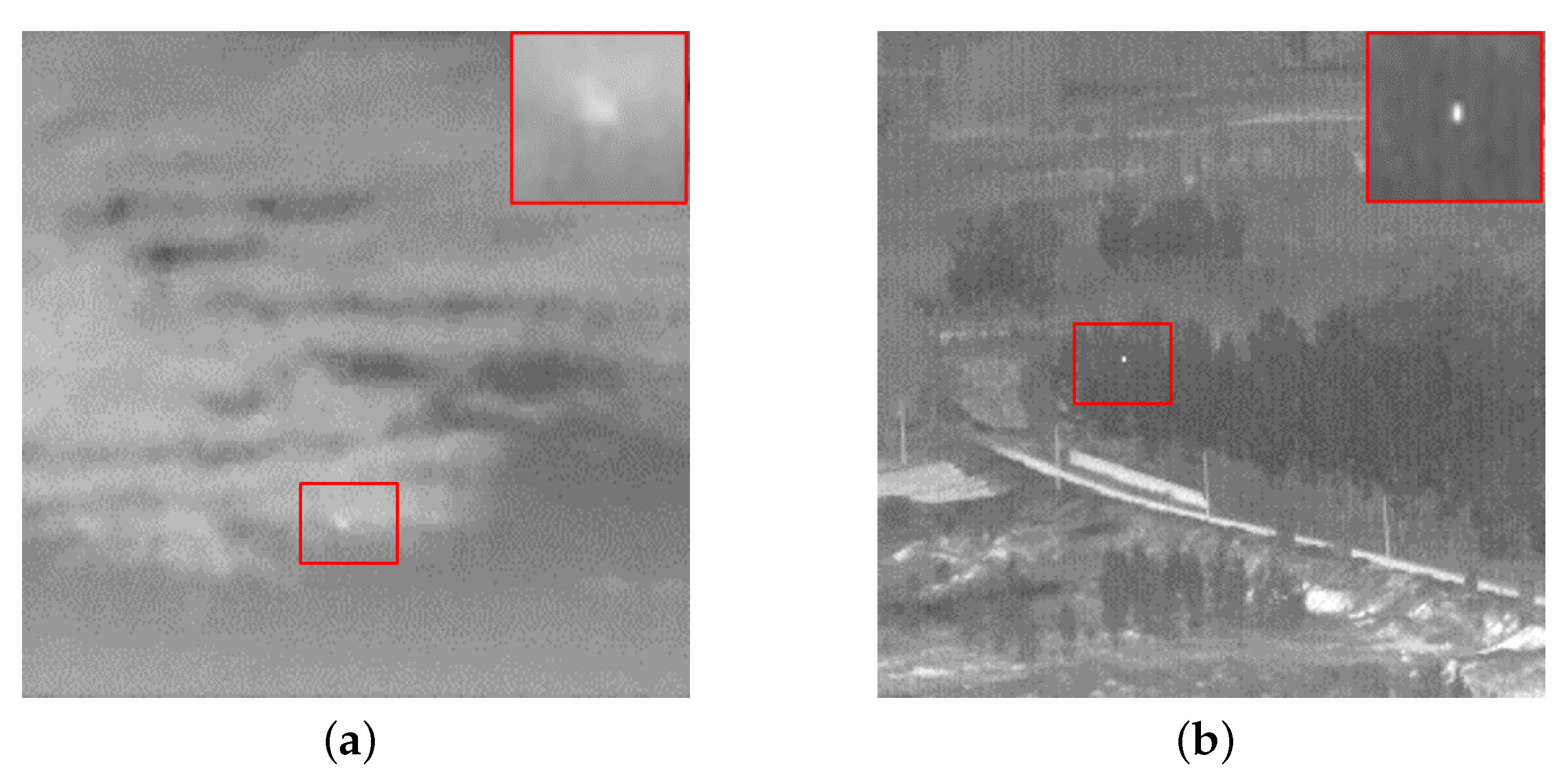
Figure 1. The typical infrared images; (a,b) are infrared images in two different complex scenes.
Remotesensing 15 01508 g001
Figure 2. Flowchart of the proposed algorithm.
Remotesensing 15 01508 g002
Figure 3. The hierarchical gradient model and the Laplacian filter kernel; (a) is the hierarchical gradient model, and (b) is the Laplacian filter kernel.
Remotesensing 15 01508 g003
Figure 4. The image is filtered by a Laplacian; (a) is the original image and (b) is the image smoothed by the Laplacian filter kernel.
Remotesensing 15 01508 g004
Figure 5. The image is filtered by the proposed method; (a) is the original image, (b) is the image after smoothing by the preprocessing algorithm, and (c) is the traditional RGM after only Laplacian filtering. (d) is the RGM obtained by the proposed method.
Remotesensing 15 01508 g005
Figure 6. An introductory figure of the local background region of the target. The red box is the position of the target, and the yellow box is the local background area of the target. The size of the local background area in the figure is (x + 2b)∗(y + 2b).
Remotesensing 15 01508 g006
Figure 7. An introduction to the three-layer window model.
Remotesensing 15 01508 g007
Figure 8. Variance difference at different regions; (a) is the infrared image, and the yellow numbers in (b) are the variances of different regions in (a).
Remotesensing 15 01508 g008
Figure 9. The effect of the proposed method. (a) is the PRT obtained by the LCF, (b) is the PRT obtained by the LV, and (c) is the PRT obtained by the proposed algorithm. The red marks are the target components that we want to highlight. The green marks are false alarm components that we do not want to highlight.
Remotesensing 15 01508 g009
Figure 10. Different imaging sizes of the same target; (a) is the image collected when the target distance is close, and (b) is the image collected when the target is far away.
Remotesensing 15 01508 g010
Figure 11. The relationship between the target and the background; 255 in green, 210 in blue, 150 in gray, and 10 in light color represent the target, bright background, transition region and dark background, respectively. (ad), respectively, represent the target in the dark background area, a small amount of noise area, transition area, and the bright background area.
Remotesensing 15 01508 g011
Figure 12. The intensity curves for different types of pixels in the time domain; (a) is a typical infrared image and different colors mark different pixel areas, (b) is the sequence information, and (c) is the temporal intensity curve.
Remotesensing 15 01508 g012
Figure 13. 3-D curves of parametric analysis, showing detection probability versus the false alarm rate and the parameter vs. in Equation (22). In the legends, the corresponding AUCS are shown. (a) S represents the scale size of the window, (b) K represents the scale size of the sub-window, and (c) the sizes of m 1 and m 2 represent different weights and m 2 is fixed at 1.
Remotesensing 15 01508 g013
Figure 14. 3-D curves of ablation experiments, showing detection probability versus the false alarm rate and the parameter vs. in Equation (22). In the legends, the corresponding AUCS are shown. The “-” in the legend is the experiment performed by removing a certain part of the proposed algorithm. (a,b) are experimental results obtained in data 1 and data 2, respectively.
Remotesensing 15 01508 g014
Figure 15. Detection results of one frame in data1. The first sub-image is the original image, and the rest are the detection results of each algorithm.
Remotesensing 15 01508 g015
Figure 16. Three-dimensional displays of detection results on one frame in data1. Different subgraphs are the results of different algorithms.
Remotesensing 15 01508 g016
Figure 17. Detection results of one frame in data2. The first sub-image is the original image, and the rest are the detection results of each algorithm.
Remotesensing 15 01508 g017
Figure 18. Three-dimensional displays of detection results on one frame in data2. Different subgraphs are the results of different algorithms.
Remotesensing 15 01508 g018
Figure 19. Detection results of one frame in data3. The first sub-image is the original image, and the rest are the detection results of each algorithm.
Remotesensing 15 01508 g019
Figure 20. Three-dimensional displays of detection results on one frame in data3. Different subgraphs are the results of different algorithms.
Remotesensing 15 01508 g020
Figure 21. 3-D ROC curves of different methods on data. (af) are the curves of data1-data6. Curves in different colors are the results of different algorithms.
Remotesensing 15 01508 g021
Figure 22. The images added noise with mean 0 and variance 0.01.
Remotesensing 15 01508 g022
Figure 23. The detection results of the proposed algorithm of Figure 22.
Remotesensing 15 01508 g023
Figure 24. The histogram of the four evaluation indicators for several methods.
Remotesensing 15 01508 g024
Table 1. The dataset contains six sequences.
DataFramesAverage SCRScene Introduction
Data 18005.45long distance, ground background, long time
Data 23996.07ground background, alternating near and far
Data 35003.42Target maneuver, ground background
Data 44003.84Irregular movement of target, ground background
Data 54003.01Target maneuver, sky ground background
Data 64002.20Target from far to near, single target, ground background
Table 2. The experimental parameters.
MethodsParameter Settings
LCM [13]window size: 3∗3
MPCM [14]window size: 3∗3, 5∗5, 7∗7, mean filter size: 3 ∗ 3
RLCM [15](K1, K2) = (2, 4), (5, 9), and (9, 16)
DNGM [18]sub-window size: 3∗3
STLDM [30]frames = 5
TLLCM [17]Gaussian filter kernel
VAR-DIFF [23]window size: 3∗3, 5∗5, 7∗7
WSLCM [21]window size: 3∗3, 5∗5, 7∗7, 9∗9
WTLLCM [20]sub-window size: 3∗3, K = 4
Proposedsub-window size: 3∗3, K = 2, m 1 = 2, m 2 = 1
Table 3. Measurements for ten detection methods.
MethodsSeq.1Seq.2Seq.3
BSFSCRGAUCBSFSCRGAUCBSFSCRGAUC
LCM0.4811.8420.1080.4971.8160.2030.8195.3310.054
MPCM2.4051.79104.0946.3710.2525.4033.5810.010
RLCM1.1173.6370.052.2243.8220.1122.6372.3000.010
DNGM4.6074.0330.0447.9022.1420.27210.2401.9410
STLDM5.5654.7020.6548.5933.4060.9306.3813.6320.457
TLLCM3.7442.4860.1536.2241.8480.1288.4921.8270.149
VAR-DIFF4.89516.0610.0017.48711.910.18910.7983.0010.001
WSLCM5.81811.0730.0098.4603.0710.1699.5263.3980.086
WTLLCM5.19411.4880.17010.2854.7710.63210.1712.1810.020
Proposed577.223.1620.8561805.95.8230.95537.2886.9340.893
Table 4. Measurements for ten detection methods.
MethodsSeq.4Seq.5Seq.6
BSFSCRGAUCBSFSCRGAUCBSFSCRGAUC
LCM1.7552.0870.1391.6251.0040.1122.1047.4180.315
MPCM12.9860.1600.81416.6742.6030.8999.8930.0100.022
RLCM14.7150.5830.1749.1431.3020.2353.4173.9810.074
DNGM20.2322.2220.88045.6932.1250.95214.5271.1290.001
STLDM18.6812.0860.96318.9391.9880.85519.35818.5880.883
TLLCM31.5762.5480.99928.1432.6760.94313.8441.2700.001
VAR-DIFF15.1641.1790.75646.2452.9560.89318.4922.3860.001
WSLCM56.6791.8620.997117.642.1270.95322.0170.9990.005
WTLLCM23.7712.4010.93197.4672.4040.92016.6630.7050.030
Proposed2355.21.7850.9973247.41.8150.980375.1619.9450.978
Table 5. Computation time of different methods.
MethodsSeq.1(/s)Seq.2(/s)Seq.3(/s)Seq.4(/s)Seq.5(/s)Seq.6(/s)
LCM0.0420.0570.0630.0540.0800.057
MPCM0.0370.0380.0430.0410.0410.041
RLCM4.5675.4996.2014.5253.8293.905
DNGM0.0370.0370.0430.0390.0370.039
STLDM1.6291.6181.6091.6271.6071.693
TLLCM1.1471.1291.1521.0871.0841.090
VAR-DIFF0.0100.0120.0140.0090.0090.013
WSLCM4.5704.4774.5794.4154.4615.192
WTLLCM0.3270.2660.2880.2760.2960.316
Proposed0.9990.9931.0100.9630.9730.994
Disclaimer/Publisher’s Note: The statements, opinions and data contained in all publications are solely those of the individual author(s) and contributor(s) and not of MDPI and/or the editor(s). MDPI and/or the editor(s) disclaim responsibility for any injury to people or property resulting from any ideas, methods, instructions or products referred to in the content.