Abstract
Monitoring the Earth’s surface and objects is important for many applications, such as managing natural resources, crop yield predictions, and natural hazard analysis. Remote sensing is one of the most efficient and cost-effective solutions for analyzing land-use and land-cover (LULC) changes over the Earth’s surface through advanced computer algorithms, such as classification and change detection. In the past literature, various developments were made to change detection algorithms to detect LULC multitemporal changes using optical or microwave imagery. The optical-based hyperspectral highlights the critical information, but sometimes it is difficult to analyze the dataset due to the presence of atmospheric distortion, radiometric errors, and misregistration. In this work, an artificial neural network-based post-classification comparison (ANPC) as change detection has been utilized to detect the muti-temporal LULC changes over a part of Uttar Pradesh, India, using the Hyperion EO-1 dataset. The experimental outcomes confirmed the effectiveness of ANPC (92.6%) as compared to the existing models, such as a spectral angle mapper (SAM) based post-classification comparison (SAMPC) (89.7%) and k-nearest neighbor (KNN) based post-classification comparison (KNNPC) (91.2%). The study will be beneficial in extracting critical information about the Earth’s surface, analysis of crop diseases, crop diversity, agriculture, weather forecasting, and forest monitoring.
1. Introduction
Remote sensing is one of the efficient ways to monitor and manage natural resources and prediction analysis. Some examples are crop yield estimation [1], soil erosion detection [2], urban planning [3], forest mapping [4], and climate variability [5]. Change detection is important for observing the multitemporal changes over the Earth’s surface and detecting ground objects using optical or/and microwave remote sensing. The optical spectral bands, i.e., visible near-infrared (VIS-NIR) and shortwave infrared (SWIR), are a good source of information to retrieve critical information from the Earth’s surface [6]. In recent decades, numerous multispectral sensors have flown into space for earth observations [7]. However, the multispectral sensor’s detection, identification, and quantification of surface materials is the challenge. In such situations, the hyperspectral sensor has the potential to identify and quantify critical information, which may be possible with multispectral sensors.
Hyperspectral collects and processes information across the electromagnetic spectrum in numerous narrow bands with the potential to explore unseen information. Hyperspectral sensors are consistent and one of the richest sources of information retrieval from the Earth’s surface [8]. With the high level of spectral details, the hyperspectral provides numerous benefits, namely crop disease detection [9,10,11], leaf index estimation [12,13], object identification [14,15], and forest monitoring [16,17]. However, the implementation of computer algorithms, i.e., multitemporal change detection and classification, is challenging due to the occurrence of atmospheric distortion, radiometric errors, and misregistration between two or more multitemporal hyperspectral images [18].
The classification of remote sensing images allows the identification of various class categories and the generation of thematic maps [19]. Classification is a technique used to group the data into a specific number of classes based on pixels which can be achieved with the help of various classifiers, broadly classified as hard and soft classifiers [20]. In the past few decades, numerous classification algorithms based on machine learning and deep learning were developed for earth observation, such as support vector machine (SVM) [21,22], random forest (RF) [23,24,25], and artificial neural network (ANN) [26]. The classification of hyperspectral data is one of the challenging tasks due to the intrinsically nonlinear problem and hindrance in extracting features. Therefore, choosing the classifier for hyperspectral imagery is crucial for efficient change detection analysis [27,28].
Change detection is used to identify multitemporal variations by observing them at two or more time intervals. The significant applications of change detection involved monitoring crop stress [29,30], deforestation [31], vegetation changes, season assessment, LULC change analysis, etc. [32]. Numerous change detection techniques were developed in the literature, such as image differencing [33], image rationing [34], change vector analysis (CVA) [35], principal component analysis (PCA) [36], post-classification comparison (PCC) [37], artificial neural network (ANN) based PCC [38], and many more [39]. However, some challenges are still there, such as mixed pixel problems for the coarse-resolution dataset, radiometric errors and misregistration between the multi-temporal images, computation power constraints in the case of deep learning [40], and incorporation of the pan-sharpened dataset [41]. Each change detection technique has advantages and drawbacks, so selecting suitable methods depends upon various factors, such as the type of input datasets (i.e., microwave or optical), spatial resolution, spectral resolution, and pan-sharpened requirements [42]. Therefore, the continuous development of change detection techniques is always the primary requirement of researchers to detect the seasonal or annual variations over the Earth’s surface with the help of high-spectral resolution datasets due to their importance in detecting crucial materials or objects [43].
Various authors have reported the work done over LULC using different change detection techniques. Goswami et al. [44] implemented a change detection technique for multitemporal images. The decision tree algorithm with the PCC technique is proposed and compared with other change detection techniques, such as image differencing using a multispectral dataset. The author highlighted the accuracy of 91% is achieved using a decision tree with PCC techniques. Zhu et al. [45] implemented a continuous change detection algorithm using a multispectral dataset and achieved an accuracy of 90%.
Similarly, Zhang et al. [46] proposed a continuous change detection technique to monitor the forest using a multispectral dataset via an index method over the country of China. A total of three categories, namely forest, water, and others, are used, and the accuracy of the changed map was 86.4% which was achieved. A deep learning algorithm via encoder-decoder architecture is proposed by Nail et al. [47] over Karnataka for LULC detection. The accuracy was 94% using a multispectral dataset (advanced wide-field sensor (AWiFS)). Although the accuracy achieved is more than the proposed technique, it is performed on the multispectral dataset, and deep learning is used, which requires high computational power compared to the proposed technique. Liu et al. [48] proposed a semi-supervised change detection technique, namely a multilayer cascade screening strategy (MCSCD) over four different datasets, i.e., Hermiston (2004 and 2007) dataset, river dataset (2013) in China, USA dataset (2004 and 2008), and China dataset (2006 and 2007). The accuracy obtained for each dataset was different, like the Hermiston dataset (97.84%), river dataset (93.46%), USA dataset (94.46%), and China dataset (91.59%). The author claimed to achieve accuracy above 90% with slight variation according to datasets. However, this algorithm works better only for an unlabeled and smaller number of samples.
This article focuses on developing and demonstrating the potential of a simple framework to generate thematic and change maps by integrating an artificial neural network (ANN) classifier in post-classification comparison (PCC), named ANPC, using Hyperion datasets. To demonstrate the proposed work, the Earth Observation (EO-1) Hyperion dataset has been acquired in a part of Uttar Pradesh (a state of India). The major objectives of the research studies included (a) preprocessing of the input dataset; (b) generation of thematic and change maps using ANPC; (c) validation of thematic and change maps generated via ANPC; (d) comparative analysis of the proposed technique with spectral angle mapper (SAM) based post-classification comparison (SAMPC) and k-nearest neighbor (KNN) based post-classification comparison (KNNPC) techniques. It is expected that the outcome of the study allows the effective utilization of the hyperspectral dataset in the detection of identification and quantification of the inferring biological and chemical processes over the Earth’s surface.
2. Materials
Study Area
The study area is located in a part of the North Indian State, i.e., Uttar Pradesh. It is geographically located between the latitude of 27°23′23″N to 27°29′36″N and longitude of 77°24′52″E to 77°28′56″E as shown in Figure 1. The Uttar Pradesh State covers the major portion of agricultural land and contributes to the development of India. It is one of the leading states for wheat production in India [49,50]. Therefore, the continuous monitoring of agricultural land is required to protect the environment [51,52]. The major class categories involved in the study site are built-up, dense vegetation, deciduous vegetation, and others (mixed categories due to less land held by the class). The study area is vegetative, consisting of these four broader classes which can be properly classified. Some categories are limited (herbs, shrubs) and difficult to examine using satellite images, so they have been added to other categories.
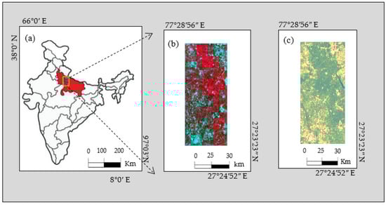
Figure 1.
Representation of study area: (a) Indian map highlights the Study area, (b) Study site using Hyperion dataset (RGB: 40:30:20), (c) Reference image.
The cloud-free EO-1 Hyperion satellite dataset was acquired on multitemporal dates, i.e., 24 February 2005 and 9 February 2014, from the United States Geological Survey (USGS) earth explorer online web platform (https://earthexplorer.usgs.gov/, accessed on 16 December 2022). The spectral resolution of EO-1 Hyperion data is 242 with the separation of narrow bandwidth, i.e., 10 nm (wavelength range of 356–2577 nm). Moreover, the spatial resolution is 30 m, having a swath width of 70 km. During image acquisition, the solar elevation and inclination angles were 135.76° and 98.07°, respectively. This dataset offers a radiometric resolution of 14 bits. Each image (band) of dimension 1061 × 3751 (2005) and 951 × 3417 (2014) is used for Hyperion EO-1 with the Geo Tiff format. The sun azimuth angle of the dataset (2005) is 139.04 and for (2014) is 135.68 and the sun elevation angle (2005) is 44.24 and for (2014) is 35.25, satellite inclination is 98.07 degrees for both, orbit path 147 and orbit row 41 for both datasets. Figure 2 represents the Hyperion EO-1 dataset acquired on multitemporal dates over the study site. To train the network and validate the outcomes, a very high-resolution dataset was acquired from the Pleiades.
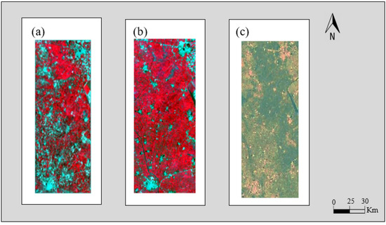
Figure 2.
Representation of reflectance images acquired using Hyperion (RGB: 40:30:20): (a) 24 February 2005, (b) 9 February 2014, (c) Reference Image.
In the training and validation processes, fine-resolution data from the Pléiades constellation, i.e., Pléiades -1A and Pléiades 1B were used. This satellite is managed by Airbus Defense and Space/Centre National d’Etudes Spatiales (CNES). It delivers high-resolution imagery, which can provide greater details about the region. ERDAS Imagine Earth Resources Data Analysis System (2015) consists of in-built google earth (GE) viewer where an image can be grounded about the GE. It offers the ability to connect to GE, travel to a specific location, match photographs to GE and vice versa, export footprints, and perform syncing. Very high-resolution remote sensing can be utilized to validate the data that the Pléiades system provides. It can be used to measure the distance between small objects like rural roads and buildings or to provide information to recognize and identify them. Farming: locating crop disease and agricultural monitoring.
3. Methods
As shown in Figure 3, the flowchart of the proposed methodology included (a) preprocessing of the hyperspectral dataset (atmospheric/radiometric corrections, bad bands removal, and strip errors correction), (b) generation of thematic and change maps using ANPC, (c) validation of thematic and change maps generated via ANPC, and (d) comparative analysis of the proposed technique with SAMPC and KNNPC technique is done.
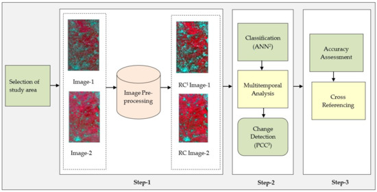
Figure 3.
The flowchart of the proposed methodology. Note: 1 RC: Radiometric Correction; 2 ANN: Artificial Neural Network; 3 PCC: Post Classification Comparison.
3.1. Preprocessing of Hyperion Dataset
The preprocessing is an essential step before change detection analysis to compensate for the atmospheric noise, radiometric distortion [53], geometric errors, and bad band [54]. The hyperspectral data, namely Hyperion EO-1, is chosen for the study purpose as it consists of a huge collection of spectral bands, i.e., 242, but 197 informatory bands are used for the present study. The bad spectral bands have been removed from the input dataset. Bad bands are unused bands that cannot be used for further processing in the dataset. These bands do not contain any information, so they are removed from the study to avoid unnecessary stacking of layers and increase computational time [48,55]. To perform the atmospheric/radiometric corrections, FLAASH (Fast Line-of-Sight Atmospheric Analysis of the Spectral Hypercubes) in the ENVI (Environment for Visualizing Images) v5.3 was utilized for hyperspectral (i.e., Hyperion) datasets to correct wavelengths in the NIR and SWIR region [56,57,58]. Afterward, an area of interest (AOI) was extracted from the input dataset.
Hyperspectral imaging is a process of extracting information from massive images at discrete wavelengths. It is a growing and hot topic in remote sensing for researchers worldwide [59]. The foremost objective of hyperspectral imaging is to attain a spectrum for each pixel in the image to find an object. However, it is an appropriate method used to detect green citrus [60], crop disease identification [31], and species diversity [61]. Moreover, it also focuses on urban analysis, land use, land cover(LULC) monitoring [62], mineral identification, management of water quality [63], etc. Hyperspectral imaging is preferred over multispectral imaging because it provides more detailed information and various applications, which is impossible via multispectral imaging. Compared to multispectral imaging, it offers various advantages such as narrower bands, higher spectral resolution, the ability to detect more than a hundred bands, distinct wavelengths, and a continuous spectrum of each pixel. These advantages favor using hyperspectral data in weather forecasting, forest monitoring, environmental monitoring, water body detection, etc.
3.2. ANPC as a Change Detection
To estimate the LULC multitemporal changes, ANPC as change detection has been utilized in the present work. It included two parts: (a) classification of input dataset using ANN classifier; and (b) generation of change maps using post-classification comparison (PCC). The ANN is one of the most reliable classification tools to resolve complex classification problems and learns through past experiences or gaining knowledge via training [64]. The simplest form of the neural network is feed-forward, but it cannot move backward and adjust weights. Therefore, a multilayer feed-forward neural network is used for the present study. Backpropagation is a supervised method used for multilayer feed-forward networks. The information processing of one or more neurons, also known as neural cells, serves as the model for feed-forward neural networks [65]. A neuron’s dendrites receive input signals before transmitting them to the cell body. The signal is sent from the cell’s axon to synapses, where one cell’s axon connects to another cell’s dendrites. Similarly, the backpropagation approach’s fundamental idea is to simulate a given function by altering the internal weights of input signals to generate an anticipated output signal. The system is trained via supervised learning techniques.
The backpropagation technique is used to adjust the weights in neurons to minimize the error rate, which is obtained in the previous epochs using the recursive method. The error rate can be reduced with the help of proper weight tunning, and the model can be made more reliable. It is comprised of three layers, namely the input node, hidden layer, and output nodes. The input node initiates the input data for further processing with the help of neurons. The hidden layer is intermediate between the input and output node, where neurons are adjusted with the help of the backpropagation method [47]. The processing of ANN consists of numerous parameters, such as a single hidden layer selected with a logistic activation function, 0.80 threshold value, and 0.27 training rate with 0.65 of training momentum. It consists of 197 input nodes and four output nodes (built-up, dense-vegetation, deciduous vegetation, and others using 500 total iterations. After the predate and postdate input datasets have been categorized, PCC can produce a change map linked to “from-to” class variations. Here, only three layers are enough to make ANN a strong model with high accuracy.
The ANN model was found useful in the detection of LULC changes, food adulteration, crop disease detection [66,67], weather forecasting [68,69,70], and assessment of damage in mushrooms [71]. The ANN classifier is best suitable for the hyperspectral dataset to process and extract the crucial details. Moreover, it is a rapid algorithm to resolve classification issues. The model is trained using various categories such as vegetation, built-up, and crop analysis [72]. The hyperspectral dataset is linked with the reference dataset using the inbuilt Google Earth tool in Earth Resources Data Analysis System (ERDAS) version 2015 for analyzing various features related to the study area. A total of 1000 samples are used for the study purpose, further categorized into training (~80%) and testing (~20%). During training, the input image is selected. The region of interest (ROI) is chosen for training consisting of different classes such as built-up, dense vegetation, deciduous vegetation, and minor crops (others). After completion of model training, implementation is performed over images. The dataset is preprocessed and classified using ENVI (Environment for Visualizing Images) v5.3 software. If testing accuracy is higher, then the model does not suffer from an overfitting problem [73]. If the desired output is not produced, then the model refinement can be done by choosing an ROI having a prominent number of pixels [74]. After the computation of thematic maps from ANN of each input dataset, the PCC as change detection has been implemented over multitemporal thematic maps generated from the hyperspectral dataset using the ERDAS software version 2015 [75,76].
Change detection is a technique used to measure the changes between multitemporal images or areas within a specified period. In the past literature, numerous authors have implemented different change detection techniques, namely image differencing, image rationing [77], post-classification comparison (PCC) [78,79,80], change vector analysis, etc. [81]. However, PCC is the best classification change detection among them all. This change detection method allows pixel-wise comparison and restricts the requirement of strict radiometric. The accuracy of PCC is highly dependent on the quality of the classified map; thus, the classified maps need to be accurately classified. PCC is a commonly used changed detection method, straightforward and easily applicable to all sensor images irrespective of the same environmental condition [82,83].
3.3. Cross-Referencing
To compare the outcomes of the proposed technique, two well-defined techniques, i.e., SAMPC and KNNPC, have been implemented. SAM is also a supervised classification method based on the assumption that a single pixel on the image represents one class category. In this, the spectra of the image are compared with known spectra. This is used to discover similarities between variant spectra via calculating the spectra angle between them. Here, a smaller angle means a near match to the referred spectrum. It has been widely used with remote sensing datasets. However, it is not useful for the hyperspectral dataset because of angle calculation for multiple spectral bands, which makes it a cumbersome method for the high-dimensional dataset. On the other hand, KNN is a flexible classifier that can be used for classification and regression. There is no special training required for this algorithm; it is also known as the lazy algorithm [84,85,86,87]. This classifier outperforms the SAM model and is best for a limited training dataset, though, in the case of a higher training dataset, it will not achieve higher accuracy. After the computation of thematic maps from SAM and KNN of each input dataset, the PCC as change detection has been implemented over multitemporal thematic maps; thus, the technique is named SAMPC and KNNPC, respectively.
3.4. Accuracy Assessment
The validation of thematic and change maps is required to evaluate the efficacy of the proposed model. Each thematic and change map has been compared with the reference dataset, i.e., Pleiades images of the precise region. For the validation, more than 100 pixels have been selected for each class or conversion category. The evaluation metrics used to find the accuracy of the proposed model are (a) producer’s accuracy (PA), referring to the correct classified pixel on the image from the user’s point of view, (b) user’s accuracy (UA), referring to the classification of the pixel on the image representing the same value on the ground, (c) omission error (OE), representing the probability of the reference pixel to be accurately classified, (d) commission error (CE) representing the incorrect classification of the classified classes, (e) overall accuracy (OA) representing the mapping of the reference site with classified categories, and (f) kappa coefficient (Kc), including the difference between the actual and the expected outcome [88].
4. Results and Discussion
The ANPC has been implemented to detect the muti-temporal LULC changes over a part of Uttar Pradesh, India, using the Hyperion dataset. The outcomes of the ANPC have also been compared with SAMPC and KNNPC. In the initial stage, each input dataset, i.e., 24 February 2005 and 9 February 2014, has been classified using different classification algorithms, i.e., ANN, SAM, and KNN. Figure 4 represents the classified maps generated from different classification algorithms, i.e., ANN, SAM, and KNN.
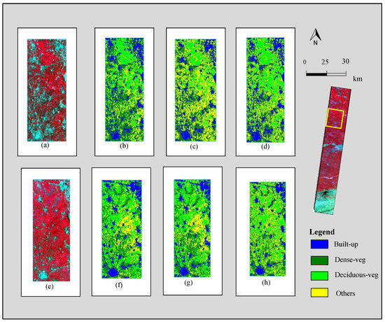
Figure 4.
Classified map of: (a) Hyperion imagery (24 February 2005) computed from (b) ANN (c) KNN (d) SAM; (e) Hyperion imagery (9 February 2014) computed from (f) ANN (g) KNN (h) SAM.
Notably, the present scenario has selected four class categories, i.e., built-up, dense vegetation, deciduous vegetation, and minor crops (others). ANPC, SAMPC, and KNNPC have been implemented to generate the change map. The experimental analysis uses hardware configuration: Windows 10/11, mac OS 10.14, and above. Approximately 4 GB of disk space is required for software installation, 4-core Intel Xeon W-2104 @3.2 GHz, NVIDIA Quadro P620 2 GB. Software platform: NVIDIA graphics card with CUDA Compute Capability is required for ENVI v5.3 platform, which is required for classification; ERDAS 2015 is required for analysis purposes, and Google Earth for validation. Currently, fewer epochs (20) have been chosen because of the limited computation resources, which lengthens the running duration. However, if plenty of computing resources are available, the running duration can be increased by choosing a lot of epochs. Since topology, training methods, and other factors may vary from application to application, and yet are adaptable, there is no standard approach for identifying the machine learning parameters.
In each change map, twelve class-conversion categories exist. The statistical analysis has also been computed for each classified and change map, as shown in Table 1 and Table 2, respectively, highlights the various parameters such as producer accuracy (PA), user accuracy (UA), overall accuracy (OA), and kappa coefficient (Kc).

Table 1.
Accuracy Assessment of ANN, SAM, and KNN classification of Hyperion EO-1.
Table 2.
Accuracy Assessment of change maps computed from SAMPC, KNNPC, and ANPC using Hyperion.
From Hyperion classified results (Table 2), it has been observed that ANN outperforms and achieved OA of (94.50–94.80%) as compared to SAM (91.10%–91.40%) and KNN (93.00%–93.30%). From Table 2, it has been concluded from the results that ANPC outperformed with an accuracy of (92.60%) as compared to SAMPC (89.70%) and KNNPC (91.30%).
In addition, the changed areas have also been calculated from ANPC, SAMPC, and KNNPC using Hyperion datasets, as shown in Table 3. From visual and statistical analysis, it has been observed that Hyperion EO-1 is capable of fetching precise information due to the large number of narrow bands which may use in the categorization of various class categories. Past literature states that extensive work has been done using multispectral datasets through numerous classifiers [89]. Despite various benefits, the multispectral dataset is not capable of producing the desired outcome because of a limited wider band. Some studies have shown remote sensing applicability using hyperspectral datasets over water bodies and wetlands, plant diseases, and forest monitoring.
Table 3.
Representation of change area (in percentage) computed from SAMPC, SVMPC, and ANPC using Hyperion EO-1.
The present study proposed a simple framework, ANPC, to detect the changes in the LULC area. The proposed method has improved accuracy compared with other state-of-art algorithms, i.e., SAMPC and KNNPC. This work has demonstrated that, in comparison to KNNPC and SAMPC, the proposed technique ANPC enhanced efficiency by extending the application of the hyperspectral dataset in identifying land surface changes. The underlying cause of these results may be that KNNPC is computationally inefficient and excels only with prediction problems, while SAMPC excels only with a limited set of spectral bands. Compared to both, ANPC performs well with images, is connected to various neurons, and is regarded as a quick and simple algorithm to learn. Compared to KNNPC and SAMPC, it can also extract more features because of hidden layers. Figure 5 represents the visual analysis of various classified maps, and Figure 6 portrays the changed and non-changed areas using different classifiers. The results of the experiments have demonstrated that the ANPC approach is quicker and more efficient at evaluating modified maps.
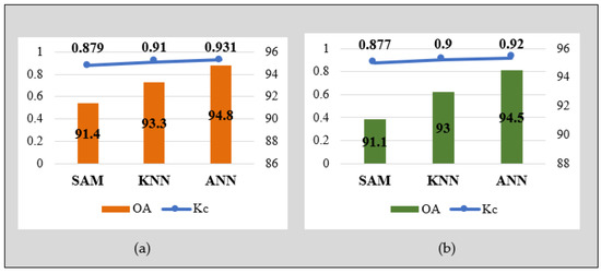
Figure 5.
Comparison of accuracy assessment of classified maps computed from (a) Hyperion EO-1 (2005), (b) Hyperion EO-1 (2014).
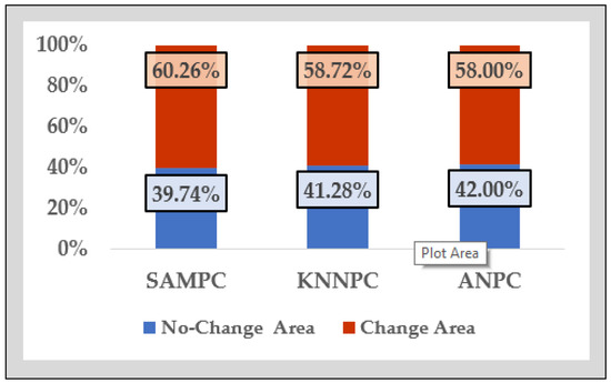
Figure 6.
Graphical representation of “change/no-change” area computed from different change detection methods, i.e., SAMPC, SVMPC, and ANNPC, using Hyperion EO-1.
The ANPC technique is better and more effective at evaluating changed maps because of backpropagation, which helps manage error by adjusting weights and improving the accuracy KNNPC performs well with a small number of the dataset, and SAMPC suffers from the albedo effect means the surface’s ability to reflect sunlight. The experimental results have shown that the ANPC approach is faster and finer than SAMPC and KNNPC. Moreover, the proposed technique can also be explored for other areas such as weather forecasting, leaf index, crop identification, etc. The proposed ANPC technique has also shown improved accuracy compared with other stated algorithms in the literature. Goswami et al. [44] implemented a change detection technique for a multitemporal image with 91% accuracy, which is lesser than the proposed method and can detect fewer spectral bands only. Zhu et al. [45] implemented continuous change detection and classification (CCDC) algorithm using a multispectral dataset and achieved an accuracy of 90%, which is less than the proposed technique and not applicable to higher resolution datasets, which is a part of the pre-classification technique. Similarly, Zhang et al. [46] also proposed a continuous change detection technique and achieved an accuracy of 86.4% which is lesser than the proposed method. Nail et al. [47] used deep learning over LULC and achieved 94% accuracy. Currently, we have focused only on post-classification techniques with limited datasets per availability. We will also focus on new techniques like CCDC and advanced deep learning techniques in the future.
The proposed technique is specially designed for the hyperspectral dataset using post-classification techniques. However, this technique can be used for other satellites and the latest datasets. Due to data unavailability, testing of the technique is done on a smaller scale, but in the future, we will also work on a larger scale with the latest datasets and fusion with other methods.
5. Conclusions
In this paper, the potential of the hyperspectral dataset, i.e., Hyperion EO-1, is evaluated in estimating LULC multitemporal changes using a straightforward ANPC change detection approach. This study was conducted in a part of Uttar Pradesh (a state of India). The experimental outcome of the ANPC has also been compared with other state-of-art algorithms, i.e., SAMPC and KNNPC. From the experiment, it is apparent that the ANPC performed well enough (92.60%) as compared to SAMPC (89.70%) and KNNPC (91.30%). However, it has also been observed that the accuracy of Hyperion EO-1 has been affected due to misclassification errors. To resolve these issues, deep learning models can be used, which will be included in future work. Although, the present work confirms the effectiveness of the ANPC in recognition of various land cover categories via hyperspectral imagery. It is expected that this work could be used for other applications such as plant disease detection, crop growth monitoring, crop yield, and leaf area index. The proposed technique can also be used for other non-decommissioned platforms. Due to the unavailability of the free dataset, the processing is performed on a limited choice of requirements. As a future work, larger scale computational can be considered using deep learning techniques.
Author Contributions
Conceptualization, N.D., S.S., S.G. and A.R.; methodology, A.S. (Adel Sulaiman), M.A.E., M.H. and A.S. (Asadullah Shaikh); software, N.D., S.S., S.G. and A.R; validation, A.S. (Adel Sulaiman), M.A.E., M.H. and A.S. (Asadullah Shaikh); formal analysis, S.S. and A.R.; investigation, N.D. and A.S. (Asadullah Shaikh); resources, A.S. (Adel Sulaiman) and M.A.E.; data curation, N.D., M.H. and A.R.; writing—original draft preparation, N.D., S.S., S.G. and A.R.; writing—review and editing, A.S. (Adel Sulaiman), M.A.E., M.H. and A.S. (Asadullah Shaikh); visualization, A.S. (Adel Sulaiman); supervision, A.S. (Asadullah Shaikh); project administration, N.D., A.S. (Adel Sulaiman) and S.G.; funding acquisition, M.A.E. All authors have read and agreed to the published version of the manuscript.
Funding
The authors would like to acknowledge the support of the Deputy for Research and Innovation, Ministry of Education, Kingdom of Saudi Arabia, for this research through a grant (NU/IFC/2/SERC/-/48) under the Institutional Funding Committee at Najran University, Kingdom of Saudi Arabia.
Data Availability Statement
Not applicable.
Conflicts of Interest
The authors declare no conflict of interest.
References
- Lu, D.; Li, G.; Moran, E. Current situation and needs of change detection techniques. Int. J. Image Data Fusion 2014, 5, 13–38. [Google Scholar] [CrossRef]
- Arefin, R.; Meshram, S.G.; Santos, C.A.G. Comparison of land use/land cover change of fused image and multispectral image of landsat mission: A case study of Rajshahi, Bangladesh. Environ. Earth Sci. 2021, 80, 1–16. [Google Scholar] [CrossRef]
- Marsal-Llacuna, M.-L.; López-Ibáñez, M.-B. Smart Urban Planning: Designing Urban Land Use from Urban Time Use. J. Urban Technol. 2014, 21, 39–56. [Google Scholar] [CrossRef]
- Puissant, A.; Rougier, S.; Stumpf, A. Object-oriented mapping of urban trees using random forest classifiers. Int. J. Appl. Earth Obs. Geoinformat. 2014, 26, 235–245. [Google Scholar] [CrossRef]
- Lv, Z.; Liu, T.; Shi, C.; Benediktsson, J.A.; Du, H. Novel Land Cover Change Detection Method Based on k-Means Clustering and Adaptive Majority Voting Using Bitemporal Remote Sensing Images. IEEE Access 2019, 7, 34425–34437. [Google Scholar] [CrossRef]
- He, C.; Wei, A.; Shi, P.; Zhang, Q.; Zhao, Y. Detecting land-use/land-cover change in rural–urban fringe areas using extended change-vector analysis. Int. J. Appl. Earth Obs. Geoinformat. 2011, 13, 572–585. [Google Scholar] [CrossRef]
- Yokoya, N.; Grohnfeldt, C.; Chanussot, J. Hyperspectral and Multispectral Data Fusion: A comparative review of the recent literature. IEEE Geosci. Remote Sens. Mag. 2017, 5, 29–56. [Google Scholar] [CrossRef]
- Lu, B.; Dao, P.D.; Liu, J.; He, Y.; Shang, J. Recent advances of hyperspectral imaging technology and applications in agriculture. Remote Sensing 2020, 12, 2659. [Google Scholar] [CrossRef]
- Im, J.; Jensen, J.R. Hyperspectral Remote Sensing of Vegetation. Hyperspectral Remote Sens. Veg. 2016, 6, 1943–1961. [Google Scholar] [CrossRef]
- Lupo, F.; Reginster, I.; Lambin, E.F. Monitoring land-cover changes in West Africa with SPOT Vegetation: Impact of natural disasters in 1998–1999. Int. J. Remote Sens. 2001, 22, 2633–2639. [Google Scholar] [CrossRef]
- Nijhawan, R.; Raman, B.; Das, J. Meta-Classifier Approach with ANN, SVM, Rotation Forest, and Random Forest for Snow Cover Mapping; Springer: Singapore, 2018; Volume 704. [Google Scholar] [CrossRef]
- Berterretche, M.; Hudak, A.T.; Cohen, W.B.; Maiersperger, T.K.; Gower, S.T.; Dungan, J. Comparison of regression and geostatistical methods for mapping Leaf Area Index (LAI) with Landsat ETM+ data over a boreal forest. Remote Sens. Environ. 2005, 96, 49–61. [Google Scholar] [CrossRef]
- Cap, H.Q.; Suwa, K.; Fujita, E.; Kagiwada, S.; Uga, H.; Iyatomi, H. A deep learning approach for on-site plant leaf detection. In Proceedings of the 2018 IEEE 14th International Colloquium on Signal Processing and its Application, CSPA 2018, Penang, Malaysia, 9–10 March 2018; pp. 118–122. [Google Scholar] [CrossRef]
- Blaschke, T. Object-based contextual image classification built on image segmentation. In Proceedings of the 2003 IEEE Workshop on Advances in Techniques for Analysis of Remotely Sensed Data, Greenbelt, MD, USA, 27–28 October 2004; pp. 113–119. [Google Scholar] [CrossRef]
- Amini, S.; Homayouni, S.; Safari, A.; Darvishsefat, A.A. Object-based classification of hyperspectral data using Random Forest algorithm. Geo-Spat. Inf. Sci. 2017, 21, 127–138. [Google Scholar] [CrossRef]
- Puletti, N.; Camarretta, N.; Corona, P. Evaluating EO1-Hyperion capability for mapping conifer and broadleaved forests. Eur. J. Remote Sens. 2016, 49, 157–169. [Google Scholar] [CrossRef]
- Allen, T. Application of spherical statistics to change vector analysis of landsat data southern appalachian spruce–Fir forests. Remote Sens. Environ. 2000, 74, 482–493. [Google Scholar] [CrossRef]
- Vivekananda, G.; Swathi, R.; Sujith, A. Multi-temporal image analysis for LULC classification and change detection. Eur. J. Remote Sens. 2020, 54, 189–199. [Google Scholar] [CrossRef]
- Liu, D.; Xia, F. Assessing object-based classification: Advantages and limitations. Remote Sens. Lett. 2010, 1, 187–194. [Google Scholar] [CrossRef]
- Dahiya, N.; Gupta, S.; Singh, S. A Comparative Analysis of Different Land-use and Land-cover Classifiers using Hyperspectral Data. In Proceedings of the 2021 IEEE 4th International Conference on Computing, Power and Communication Technologies, GUCON 2021, Kuala Lumpur, Malaysia, 24–26 September 2021. [Google Scholar] [CrossRef]
- Li, Y.; Xie, P.; Tang, Z.; Jiang, T.; Qi, P. SVM-Based Sea-Surface Small Target Detection: A False-Alarm-Rate-Controllable Approach. IEEE Geosci. Remote Sens. Lett. 2019, 16, 1225–1229. [Google Scholar] [CrossRef]
- Fauvel, M.; Benediktsson, J.A.; Chanussot, J.; Sveinsson, J.R. Spectral and spatial classification of hyperspectral data using SVMS and morphological profiles. IEEE Trans. Geosci. Remote Sens. 2008, 46, 3804–3814. [Google Scholar] [CrossRef]
- Cao, G. Cascaded Random Forest for Hyperspectral. IEEE J. Sel. Top. Appl. Earth Obs. Remote Sens. 2018, 11, 1082–1094. [Google Scholar]
- Lee, D.D.; Garnett, R.; Lawrence, N.D. Advances in Neural Information Processing Systems 25. In Proceedings of the 26th Annual Conference on Neural Information Processing Systems 2012, NIPS 2012’, Lake Tahoe, NA, USA, 3–6 December 2012; Volume 4. [Google Scholar]
- Ham, J.; Chen, Y.; Crawford, M.M.; Ghosh, J. Investigation of the random forest framework for classification of hyperspectral data. IEEE Trans. Geosci. Remote Sens. 2005, 43, 492–501. [Google Scholar] [CrossRef]
- Blum, A.L.; Rivest, R.L. Training a 3-node neural network is NP-complete. In Proceedings of the 1st Annual Workshop on Computational Learning Theory, COLT 1988, Cambridge, MA, USA, 3–5 August 1988; Volume 5, pp. 9–18. [Google Scholar] [CrossRef]
- Matthews, J.A. Land-Change Science; Sage Knowledge: Thousand Oaks, CA, USA, 2014. [Google Scholar] [CrossRef]
- Krishna, G.; Sahoo, R.N.; Pradhan, S.; Ahmad, T.; Sahoo, P.M. Hyperspectral satellite data analysis for pure pixels extraction and evaluation of advanced classifier algorithms for LULC classification. Earth Sci. Inform. 2017, 11, 159–170. [Google Scholar] [CrossRef]
- Bauer, M.E. The role of remote sensing in determining the distribution and yield of crops. In Advances in Agronomy; Brady, N.C., Ed.; Academic Press: Cambridge, MA, USA, 1975; Volume 27, pp. 271–304. [Google Scholar] [CrossRef]
- Estep, L.; Terrie, G.; Davis, B. Crop stress detection using AVIRIS hyperspectral imagery and artificial neural networks. Int. J. Remote Sens. 2004, 25, 4999–5004. [Google Scholar] [CrossRef]
- Caballero, D.; Calvini, R.; Amigo, J.M. Hyperspectral imaging in crop fields: Precision agriculture. Data Handl. Sci. Technol. 2019, 32, 453–473. [Google Scholar] [CrossRef]
- Singh, A. Review Article Digital change detection techniques using remotely-sensed data. Int. J. Remote Sens. 1989, 10, 989–1003. [Google Scholar] [CrossRef]
- Prakash, A.; Gupta, R.P. Land-use mapping and change detection in a coal mining area—A case study in the Jharia coalfield, India. Int. J. Remote Sens. 1998, 19, 391–410. [Google Scholar] [CrossRef]
- Stow, D.A.; Collins, D.; McKinsey, D. Land use change detection based on multi-date imagery from different satellite sensor systems. Geocarto Int. 1990, 5, 3–12. [Google Scholar] [CrossRef]
- Singh, S.; Talwar, R. A comparative study on change vector analysis. Sadhana 2014, 39, 1311–1331. [Google Scholar] [CrossRef]
- Rédei, G.P. PCA (principal component analysis). Encycl. Genet. Genom. Proteom. Inform. 2008, 1457. [Google Scholar] [CrossRef]
- Zheng, Z.; Cao, J.; Lv, Z.; Benediktsson, J.A. Spatial–spectral feature fusion coupled with multi-scale segmentation voting decision for detecting land cover change with VHR remote sensing images. Remote Sens. 2019, 11, 1903. [Google Scholar] [CrossRef]
- Singh, S.; Tiwari, R.K.; Sood, V.; Gusain, H.S. Detection and validation of spatiotemporal snow cover variability in the Himalayas using Ku-band (13.5 GHz) SCATSAT-1 data. Int. J. Remote Sens. 2020, 42, 805–815. [Google Scholar] [CrossRef]
- Lu, D.; Mausel, P.; Brondízio, E.; Moran, E. Change detection techniques. Int. J. Remote Sens. 2004, 25, 2365–2401. [Google Scholar] [CrossRef]
- Dahiya, N.; Gupta, S.; Singh, S. Quantitative Analysis of Different Land-use and Land-cover Classifiers using Hyperspectral Dataset. In Proceedings of the IEEE International Conference Image Information Processing, Shimla, India, 26–28 November 2021; pp. 256–260. [Google Scholar] [CrossRef]
- Kwan, C.; Budavari, B.; Dao, M.; Zhou, J. New sparsity based pansharpening algorithms for hyperspectral images. In Proceedings of the 2017 IEEE 8th Annual Ubiquitous Computing, Electronics and Mobile Communication Conference, UEMCON 2017, New York, NY, USA, 19–21 October 2017; pp. 88–93. [Google Scholar] [CrossRef]
- Sood, V.; Gusain, H.S.; Gupta, S.; Singh, S. Topographically derived subpixel-based change detection for monitoring changes over rugged terrain Himalayas using AWiFS data. J. Mt. Sci. 2021, 18, 126–140. [Google Scholar] [CrossRef]
- Chen, J.; Gong, P.; He, C.; Pu, R.; Shi, P. Land-use/land-cover change detection using improved change-vector analysis. Photogramm. Eng. Remote Sens. 2003, 69, 369–379. [Google Scholar] [CrossRef]
- Goswami, A.; Sharma, D.; Mathuku, H.; Gangadharan, S.M.P.; Yadav, C.S.; Sahu, S.K.; Pradhan, M.K.; Singh, J.; Imran, H. Change Detection in Remote Sensing Image Data Comparing Algebraic and Machine Learning Methods. Electronics 2022, 11, 431. [Google Scholar] [CrossRef]
- Zhu, Z.; Woodcock, C.E. Continuous change detection and classification of land cover using all available Landsat data. Remote Sens. Environ. 2014, 144, 152–171. [Google Scholar] [CrossRef]
- Zhang, Y.; Wang, L.; Zhou, Q.; Tang, F.; Zhang, B.; Huang, N.; Nath, B. Continuous Change Detection and Classification—Spectral Trajectory Breakpoint Recognition for Forest Monitoring. Land 2022, 11, 504. [Google Scholar] [CrossRef]
- Dahiya, N.; Singh, S.; Gupta, S. A Review on Deep Learning Classifier for Hyperspectral Imaging. Int. J. Image Graph. 2022, 22, 2350036. [Google Scholar] [CrossRef]
- Liu, L.; Hong, D.; Ni, L.; Gao, L. Multilayer Cascade Screening Strategy for Semi-Supervised Change Detection in Hyperspectral Images. IEEE J. Sel. Top. Appl. Earth Obs. Remote Sens. 2022, 15, 1926–1940. [Google Scholar] [CrossRef]
- Paul, S.; Kumar, D.N. Spectral-spatial classification of hyperspectral data with mutual information based segmented stacked autoencoder approach. ISPRS J. Photogramm. Remote Sens. 2018, 138, 265–280. [Google Scholar] [CrossRef]
- Luo, J.; Huang, W.; Zhao, J.; Zhang, J.; Ma, R.; Huang, M. Predicting the probability of wheat aphid occurrence using satellite remote sensing and meteorological data. Optik 2014, 125, 5660–5665. [Google Scholar] [CrossRef]
- Kamilaris, A.; Prenafeta-Boldú, F.X. Deep learning in agriculture: A survey. Comput. Electron. Agric. 2018, 147, 70–90. [Google Scholar] [CrossRef]
- Strachan, I.B.; Pattey, E.; Boisvert, J.B. Impact of nitrogen and environmental conditions on corn as detected by hyperspectral reflectance. Remote Sens. Environ. 2002, 80, 213–224. [Google Scholar] [CrossRef]
- Yang, Z.; Li, Z.; Zhu, J.; Wang, Y.; Wu, L. Use of SAR/InSAR in Mining Deformation Monitoring, Parameter Inversion, and Forward Predictions: A Review. IEEE Geosci. Remote Sens. Mag. 2020, 8, 71–90. [Google Scholar] [CrossRef]
- Mishra, V.D.; Sharma, J.K.; Singh, K.K.; Thakur, N.K.; Kumar, M. Assessment of different topographic corrections in AWiFS satellite imagery of Himalaya terrain. J. Earth Syst. Sci. 2009, 118, 11–26. [Google Scholar] [CrossRef]
- Datta, A.; Ghosh, S.; Ghosh, A. Band elimination of hyperspectral imagery using partitioned band image correlation and capacitory discrimination. Int. J. Remote Sens. 2014, 35, 554–577. [Google Scholar] [CrossRef]
- Sahoo, R.N.; Ray, S.; Manjunath, K.R. Hyperspectral remote sensing of agriculture. Curr. Sci. 2015, 108, 848–859. [Google Scholar]
- Singh, D.K.; Gusain, H.S.; Mishra, V.; Gupta, N. Snow cover variability in North-West Himalaya during last decade. Arab. J. Geosci. 2018, 11, 579. [Google Scholar] [CrossRef]
- Wang, D.; Ma, R.; Xue, K.; Loiselle, S.A. The Assessment of Landsat-8 OLI Atmospheric Correction Algorithms for Inland Waters. Remote Sens. 2019, 11, 169. [Google Scholar] [CrossRef]
- ElMasry, G.; Sun, D.-W. Principles of Hyperspectral Imaging Technology. In Hyperspectral Imaging for Food Quality Analysis and Control; Academic Press: Cambridge, MA, USA, 2010; pp. 3–43. [Google Scholar] [CrossRef]
- Okamoto, H.; Lee, W.S. Green citrus detection using hyperspectral imaging. Comput. Electron. Agric. 2009, 66, 201–208. [Google Scholar] [CrossRef]
- Mishra, P.; Asaari, M.S.M.; Herrero-Langreo, A.; Lohumi, S.; Diezma, B.; Scheunders, P. Close range hyperspectral imaging of plants: A review. Biosyst. Eng. 2017, 164, 49–67. [Google Scholar] [CrossRef]
- Dharani, M.; Sreenivasulu, G. Land use and land cover change detection by using principal component analysis and morphological operations in remote sensing applications. Int. J. Comput. Appl. 2019, 43, 462–471. [Google Scholar] [CrossRef]
- Roy, A.; Inamdar, A.B. Multi-temporal Land Use Land Cover (LULC) change analysis of a dry semi-arid river basin in western India following a robust multi-sensor satellite image calibration strategy. Heliyon 2019, 5, e01478. [Google Scholar] [CrossRef]
- Canty, M.J. Image Analysis, Classification and Change Detection in Remote Sensing: With Algorithms for ENVI/IDL and Python; CRC Press: Boca Raton, FL, USA, 2014. [Google Scholar]
- Guo, A.J.X.; Zhu, F. Spectral-Spatial Feature Extraction and Classification by ANN Supervised With Center Loss in Hyperspectral Imagery. IEEE Trans. Geosci. Remote Sens. 2018, 57, 1755–1767. [Google Scholar] [CrossRef]
- de Wit, A.; Clevers, J. Efficiency and accuracy of per-field classification for operational crop mapping. Int. J. Remote Sens. 2004, 25, 4091–4112. [Google Scholar] [CrossRef]
- Ramesh, K.N.; Chandrika, N.; Omkar, S.N.; Meenavathi, M.B.; Rekha, V. Detection of Rows in Agricultural Crop Images Acquired by Remote Sensing from a UAV. Int. J. Image Graph. Signal Process. 2016, 8, 25–31. [Google Scholar] [CrossRef]
- Waseem, K.H.; Mushtaq, H.; Abid, F.; Abu-Mahfouz, A.M.; Shaikh, A.; Turan, M.; Rasheed, J. Forecasting of Air Quality Using an Optimized Recurrent Neural Network. Processes 2022, 10, 2117. [Google Scholar] [CrossRef]
- Palakuru, M.; Adamala, S.; Bachina, H.B. Modeling yield and backscatter using satellite derived biophysical variables of rice crop based on artificial neural networks. J. Agrometeorol. 2020, 22, 41–47. [Google Scholar] [CrossRef]
- Zhang, Z.; De Wulf, R.R.; Van Coillie, F.M.B.; Verbeke, L.P.C.; De Clercq, E.M.; Ou, X. Influence of different topographic correction strategies on mountain vegetation classification accuracy in the Lancang Watershed, China. J. Appl. Remote Sens. 2011, 5, 053512. [Google Scholar] [CrossRef]
- Rojas-Moraleda, R.; Valous, N.A.; Gowen, A.; Esquerre, C.; Härtel, S.; Salinas, L.; O’Donnell, C. A frame-based ANN for classification of hyperspectral images: Assessment of mechanical damage in mushrooms. Neural Comput. Appl. 2016, 28, 969–981. [Google Scholar] [CrossRef]
- Bali, N.; Singla, A. Emerging Trends in Machine Learning to Predict Crop Yield and Study Its Influential Factors: A Survey. Arch. Comput. Methods Eng. 2021, 29, 95–112. [Google Scholar] [CrossRef]
- Kaur, H.; Koundal, D.; Kadyan, V. Image Fusion Techniques: A Survey. Arch. Comput. Methods Eng. 2021, 28, 4425–4447. [Google Scholar] [CrossRef] [PubMed]
- Singh, S.; Tiwari, R.K. Detection of Cryospheric Parameters with Artificial Neural Network over Antarctic Region using Ku-Band based ISRO’s SCATSAT-1 data. In Proceedings of the 2021 IEEE International Geoscience and Remote Sensing Symposium IGARSS, Brussels, Belgium, 11–16 July 2021; pp. 435–438. [Google Scholar] [CrossRef]
- Castellana, L.; D’Addabbo, A.; Pasquariello, G. A composed supervised/unsupervised approach to improve change detection from remote sensing. Pattern Recognit. Lett. 2007, 28, 405–413. [Google Scholar] [CrossRef]
- Chen, J.; Chen, X.; Cui, X.; Chen, J. Change vector analysis in posterior probability space: A new method for land cover change detection. IEEE Geosci. Remote Sens. Lett. 2010, 8, 317–321. [Google Scholar] [CrossRef]
- Walter, V. Object-based classification of remote sensing data for change detection. ISPRS J. Photogramm. Remote Sens. 2004, 58, 225–238. [Google Scholar] [CrossRef]
- Asokan, A.; Anitha, J. Change detection techniques for remote sensing applications: A survey. Earth Sci. Inform. 2019, 12, 143–160. [Google Scholar] [CrossRef]
- Wu, C.; Du, B.; Cui, X.; Zhang, L. A post-classification change detection method based on iterative slow feature analysis and Bayesian soft fusion. Remote Sens. Environ. 2017, 199, 241–255. [Google Scholar] [CrossRef]
- Thakkar, A.K.; Desai, V.R.; Patel, A.; Potdar, M.B. Post-classification corrections in improving the classification of Land Use/Land Cover of arid region using RS and GIS: The case of Arjuni watershed, Gujarat, India. Egypt. J. Remote Sens. Space Sci. 2017, 20, 79–89. [Google Scholar] [CrossRef]
- Nackaerts, K.; Vaesen, K.; Muys, B.; Coppin, P. Comparative performance of a modified change vector analysis in forest change detection. Int. J. Remote Sens. 2005, 26, 839–852. [Google Scholar] [CrossRef]
- Liu, S.; Marinelli, D.; Bruzzone, L.; Bovolo, F. A review of change detection in multitemporal hyperspectral images: Current techniques, applications, and challenges. IEEE Geosci. Remote Sens. Mag. 2019, 7, 140–158. [Google Scholar] [CrossRef]
- El-Hattab, M.M. Applying post classification change detection technique to monitor an Egyptian coastal zone (Abu Qir Bay). Egypt J. Remote Sens. Space Sci. 2016, 19, 23–36. [Google Scholar] [CrossRef]
- Zhang, Y. Support Vector Machine Classification Algorithm and Its Application. In Proceedings of the Information Computing and Applications: Third International Conference, ICICA 2012, Chengde, China, 14–16 September 2012; pp. 179–186. [Google Scholar] [CrossRef]
- Abdollahi, A.; Pradhan, B. Integrated technique of segmentation and classification methods with connected components analysis for road extraction from orthophoto images. Expert Syst. Appl. 2021, 176, 114908. [Google Scholar] [CrossRef]
- Rimal, B.; Rijal, S.; Kunwar, R. Comparing Support Vector Machines and Maximum Likelihood Classifiers for Mapping of Urbanization. J. Indian Soc. Remote Sens. 2019, 48, 71–79. [Google Scholar] [CrossRef]
- Huang, K.; Li, S.; Kang, X.; Fang, L. Spectral–Spatial Hyperspectral Image Classification Based on KNN. Sens. Imaging 2015, 17, 1–13. [Google Scholar] [CrossRef]
- Pal, M.; Foody, G.M. Evaluation of SVM, RVM and SMLR for accurate image classification with limited ground data. IEEE J. Sel. Top. Appl. Earth Obs. Remote Sens. 2012, 5, 1344–1355. [Google Scholar] [CrossRef]
- Singh, S.; Sood, V.; Taloor, A.K.; Prashar, S.; Kaur, R. Qualitative and quantitative analysis of topographically derived CVA algorithms using MODIS and Landsat-8 data over Western Himalayas, India. Quat. Int. 2020, 575–576, 85–95. [Google Scholar] [CrossRef]


Disclaimer/Publisher’s Note: The statements, opinions and data contained in all publications are solely those of the individual author(s) and contributor(s) and not of MDPI and/or the editor(s). MDPI and/or the editor(s) disclaim responsibility for any injury to people or property resulting from any ideas, methods, instructions or products referred to in the content. |
© 2023 by the authors. Licensee MDPI, Basel, Switzerland. This article is an open access article distributed under the terms and conditions of the Creative Commons Attribution (CC BY) license (https://creativecommons.org/licenses/by/4.0/).