Article

SAR Radiometric Calibration Based on Differential Geometry: From Theory to Experimentation on SAOCOM Imagery

by
Pasquale Imperatore
1,* and
Gerardo Di Martino
2
1
Institute for Electromagnetic Sensing of the Environment (IREA), National Research Council (CNR), 80124 Napoli, Italy
2
Department of Electrical Engineering and Information Technology, University of Naples Federico II, 80125 Napoli, Italy
*
Author to whom correspondence should be addressed.
Remote Sens. 2023, 15(5), 1286; https://doi.org/10.3390/rs15051286
Submission received: 22 December 2022 / Revised: 10 February 2023 / Accepted: 24 February 2023 / Published: 26 February 2023
(This article belongs to the Section Engineering Remote Sensing)

Abstract

:
The modeling and simulation of topography-induced imaging distortions are crucial for consistent radiometric information exploitation in current and forthcoming SAR-based Earth observation missions with a high spatial and temporal resolution, with relevance in several applications. In this paper, for the first time, we specifically investigate the compensation of topography-induced radiometric distortions affecting SAR images acquired by the L-band Argentinian satellite SAOCOM. We adopt a recently developed calibration method relying on an analytical formulation derived in the rigorous framework of the differential geometry of surfaces. We first provide an original interpretation of the analytical formulation, thus providing further insights into the relevant area-stretching-based formalism. Then, the numerical implementation of the method is specialized to systematically process the data acquired by SAOCOM sensors; hence, the resulting sensor-specific prototype solution processor is employed in this study. Finally, experiments performed over a real scenario in the southern part of Italy, characterized by large topography variations, are presented and discussed, thus elucidating the effectiveness of the adopted method applied to SAOCOM images. The adopted effective SAR calibration strategy opens up the way to its operational use in large-scale SAOCOM data processing.

1. Introduction

There are many possible sources of radiometric distortions in satellite SAR imaging systems [1]. SAR radiometric distortions can be grouped into systemic and scene-dependent ones, both affecting the ability to properly interpret the SAR data information.
Systemic radiometric distortions (e.g., antenna pattern, range spreading, etc.) are intrinsically generated by the SAR sensor structure and can be removed, insofar as quantitative information on the sensor’s system parameters is available.
By contrast, scene-dependent radiometric distortions arise from the inherent 2D imaging process of a 3D irregular ground shape, and they are inherently local in nature [2,3,4,5,6,7,8,9,10,11]. Accordingly, the 2D imaging process of an irregular relief intrinsically implies unavoidable radiometric distortions. This effect may have a significant influence on the radiometric information conveyed by SAR images, and therefore the proper rectification of topography-induced SAR imaging distortions becomes crucial for inverse-scattering model applications and land cover identification and classification [12,13,14].
It is then clear that the availability of effective methods and tools for rectifying the local radiometric distortions affecting SAR images is of crucial importance for converting SAR images into radiometric meaningful quantities, especially if they are supported by rigorous mathematical background with clear meaning and interpretation.
Recently, we have witnessed an increasing interest in the development of SAR systems operating at the L-band. Due to its inherent penetration capabilities, L-band radiation is useful for investigating backscattering from vegetated soils, in order to retrieve accurate estimates of biophysical parameters related to forest structure and biomass. In particular, L-band radar signatures contain important information about crop classification and crop biomass, thus making L-band SAR suitable for monitoring agricultural processes and, in particular, soil moisture [13,14].
In this context, we focus on the Argentinean SAOCOM mission (Satélite Argentino de Observación con Microondas) developed by Comisión Nacional de Actividades Espaciales (CONAE). It consists of two identical Low-Earth-Orbit (LEO) satellites (SAOCOM-1A and -1B), launched on 7 October 2018 and 30 August 2020. Each satellite is equipped with an L-band synthetic aperture radar (SAR) instrument operating at a frequency of 1.275 GHz, with an average altitude of 637 km and a 16 days repetition cycle (thus, the full constellation has a temporal revisit of 8 days). SAOCOM can operate in different acquisition modalities (Stripmap, TOPSAR narrow, and TOPSAR wide swath) and polarimetric modes (single, dual, quad, and compact polarization), and it is equipped with a 3.5 m by 10 m active phased-array antenna. The main goals of the SAOCOM mission specifically address environmental resource management and natural and anthropic hazards (e.g., landslides, oil patches, volcanic eruptions, forest fires, flooding, and coastal pollution) monitoring.
SAOCOM calibration and validation activities were based on external calibration combined with internal calibration, and an ad hoc antenna model was adopted. The external calibration activities aimed at characterizing the calibration constants, which were carried out during the commissioning phase of the SAOCOM-1A satellite, are discussed in [15]. In particular, these calibration activities include absolute radiometric calibration, antenna pattern verification, and noise measurements. Furthermore, an assessment of the SAR product quality carried out during the commissioning phase of SAOCOM-1B is provided in [16]. The abovementioned calibration activities, however, focus on systemic radiometric distortions.
Regarding topography-induced SAR radiometric distortions, some calibration approaches are available in the literature [2,3,4,5,6,7,8,9,10]. More recently, an effective method for radiometric calibration derived in the rigorous framework of differential geometry of the surfaces has been developed, and it exhibits important advantages [10,17]. In particular, as discussed in [10] the method essentially requires image-domain processing based on the evaluation of a scalar function, with important implications in terms of the computational burden. However, to the best of our knowledge, the compensation of local SAR radiometric distortions induced by topography for SAOCOM images hitherto has not been investigated.
Therefore, in this paper, the focus is on the modeling, computation, and compensation of topography-induced radiometric distortions affecting SAR imaging, with special emphasis on the use of SAOCOM data. In particular, this investigation relies on the analytical formulation of the recently developed method proposed in [10], and it is aimed at extending its physical interpretation and applicability. Therefore, the novelty of the present work is twofold, pertaining to both the strengthening of the theoretical understanding of the calibration framework originally proposed in [10] and the implementation and analysis of its application to SAOCOM data. More specifically, the three main contributions of this paper are:
(i)
Providing novel insights into the differential-geometry-based SAR image radiometric calibration method [10], thus clarifying the meaning of its general formulation and, accordingly, providing an original interpretation of the method’s analytical expression, thus shedding new light on the inherent area-stretching function-based formalism [10];
(ii)
Developing a software prototype to systematically process the data acquired by the SAOCOM sensor, thus extending the usability of the original method implementation;
(iii)
Providing a quantitative analysis of the effectiveness of the adopted methodology, through an experimental investigation conducted over a significant mountainous region using the data acquired by the recently launched SAOCOM satellite’s SAR sensor.
The paper is structured as follows. Section 2 introduces the mathematical background underlying the adopted radiometric calibration method. A novel geometrical interpretation of formalism is provided in Section 3. The experimental results obtained by using SAOCAM data are illustrated and discussed in Section 4. Section 5 concludes the paper.

2. Theoretical Background

This section provides an overview of the SAR image calibration method used in this investigation. Specifically, the adopted method is based on the analytical formulation of topography-induced radiometric distortions in SAR imaging that has been recently provided [10] by adopting the theoretical notions of the differential geometry of surfaces [18]. The relevant formulation incorporates a description of the ground surface shape in the 3D object space, by resorting to a suitable surface parametrization process, and a (sensor-centric) cylindrical coordinate system, whose longitudinal axis corresponds to the sensor flight direction. The sensor flight (azimuth) and slant-range directions define the SAR image space. Accordingly, r and a represent the slant-range and azimuth (continuous) coordinates in the SAR image space, respectively. The adopted cylindrical coordinate system suggests the adoption of the following parametric representation of the surface:
φ : Ω   R 2 R 3 ,   φ r , a = r c o s θ , r s i n θ , a
where Ω is the parametric domain, and r and a are the radar (parametric) range and azimuth coordinates in the image space, respectively. As a result, a certain location q r , a in the SAR image space generally corresponds to a point P = φ r , a of the 3D object space. As a result, the ground surface Φ = φ ( Ω ) results to be naturally parametrized in terms of the function θ = θ r , a , which represents the look-angle function defined in the image space (Figure 1).
Let Ω i , j be a prescribed rectangle (e.g., a pixel) in the r , a -image space, with surface area A Ω i , j , where i and j are the (discrete) coordinates of the pixel along range and azimuth directions, respectively. The corresponding ground surface portion in the 3D object space is mathematically described in terms of the transformation Φ i , j = φ ( Ω i , j ) ; thus, the ground surface area is denoted by A Φ i , j .
The normalized radar cross-section (NRCS) or scattering coefficient of a distributed target is defined as the average radar cross-section (RCS) per unit area on the ground [19,20,21,22]. It is traditionally denoted by σ 0 (sigma naught). The NRCS associated with a prescribed rectangle Ω i , j in the image domain, denoted as σ i j 0 , can be formally written as follows [10]:
σ i j 0 = β i j 0 A Ω i , j A Φ i , j
where β i j 0 is the (observable) radar brightness (also referred to as beta-naught) associated with the pixel of discrete coordinates i and j [23]. It is defined as the average RCS per unit area in the SAR (slant range, azimuth) image space. Note that the area associated with a SAR image pixel, A Ω i , j = A p i x e l , is a constant. To proceed with the energy-preserving reconstruction of the radiometric quantity of interest σ i j 0 in the SAR image domain, the predictable distortive factor A Ω i , j / A Φ i , j has to be computed and compensated for pixel by pixel. Equation (2) takes into account the local radiometric distortions in the SAR imaging system induced by the ground topography; thus, this inherent compensation ensures correct normalization and energy conservation.
According to [10], the area A Φ i , j of the illuminated patch on the ground Φ i , j can be written in the following form:
A Φ i , j = Φ i , j = φ ( Ω i , j ) d S = Ω i , j μ r , a d r d a
where the differential quantity d S = μ r , a   d r d a in (3) describes the elements of the surface area in the 3D object space. According to the metric tensor of the surface, the inherently dimensionless and positive function μ r , a has been established in the following form [10]:
μ r , a = 1 + r θ 2
where the vector θ represents the gradient of the look-angle function at position r , a in the image space, with
θ r , a = θ r r , a θ a r , a
and where the 2D operator r , a is given in terms of Cartesian coordinates in the image space.
Therefore, the area-stretching function (4) quantitatively expresses, in a simple and compact way, the inherent topography-induced (local) radiometric distortions, analytically derived in purely geometrical terms within the rigorous framework of the differential geometry of surfaces [18]. According to [10], Expression (4) is established in terms of the gradient magnitude of the look-angle function ( θ = θ θ ), uniquely defined in the image domain:
θ = θ r 2 + θ a 2
where the functional dependence on the image space position r , a of the look-angle function, its partial derivatives, and its gradient is suppressed and understood.
It is then clear that, according to the adopted formulation, the slopes of the look-angle function, rather than topographic elevation slopes [3], play a crucial role.
Furthermore, it is worth emphasizing that the area-stretching function μ arises from a metric determinant quantity [18], which is relevant to the spatial transformation between the SAR image space and the ground surface in the observed 3D object space [10]. As a result, μ describes how the image space is locally stretched as mapped on the ground surface. Conversely, factor 1 / μ (with 1 / μ < 1 ) describes the local compression (foreshortening) of the elementary ground surface area d S when it is mapped on the corresponding elementary area d r d a in the SAR image space (Figure 1).
It should be noted that the right-hand side of (3) denotes the integration of the area-stretching function μ over the area of the elemental domain Ω i , j (e.g., a pixel) in the image space (see Figure 1). As a result, the formulation in [10] is shown to be mathematically concise and amenable to a straightforward implementation.
It is worth highlighting that radiometric calibration cannot be rigorously obtained in layover regions, and it is meaningless in shadow regions [6]. Accordingly, the calibration operation is applied only to those regions for which a full radiometric compensation is achievable [10], thus discarding layover and shadow regions for which radiometric compensation becomes suboptimal and meaningless, respectively.
A topological remark is now in order. As a matter of fact, the assumption of one-to-one correspondences between the image domain and the ground surface domain does not hold as far as layover and shadow regions are concerned [24]. This characteristic pertains to the different topological nature of layover and shadow phenomena with respect to foreshortening, regardless of the inherent discretization operated by the digital imaging system. It is worth noting that, excluding layover and shadow regions, (1) constitutes a one-to-one mapping, as discussed in [10].
Finally, we address the resulting SAR-calibration processing, which is indeed easily implemented. A conceptual scheme describing the processing in the imaging domain is depicted in Figure 2. A digital elevation model (DEM) of the terrain was used to describe the Earth’s shape, and the geodetic aspects were considered through the use of rigorous transformations. First, geodetic coordinates and DEM elevation values were transformed into 3D coordinates in a geocentric Earth-centered, Earth-fixed (ECEF) reference Cartesian system [25]. Then, according to rigorous SAR geolocation, cylindrical coordinates were derived by using the range-Doppler method [26,27], so that the look-angle function defined in the image space was reconstructed on a regular grid (first box in Figure 2). Then, the computation of the radiometric distortion can be straightforwardly carried out by evaluating the partial derivatives of a scalar function (second box in Figure 2), which were the basis for the evaluation of the ground surface area using Expressions (3)–(6) (third box in Figure 2), and finally, the resulting values were used for radiometric correction according to (2) (last box in Figure 2). More details on the numerical implementation of the method can be found in [10].

3. Geometrical Interpretation of the Area-Stretching Function-Based Formalism

In this section, to provide further insights into the differential-geometry-based method for describing radiometric distortions in SAR images, originally developed in [10] and presented in Section 2, we provide an original geometrical interpretation of the relevant analytical formalism.
In particular, for a better understanding of the geometrical meaning of the area-stretching function (4), it is instructive to analyze how the general formulation is specialized to some meaningful canonical cases. First, the significance of the general analytical expression is illustrated by specializing it to an azimuth-invariant topographic surface case (Figure 3), and subsequently, the idealized flat-Earth case is discussed for comparison (Figure 4).

3.1. Azimuth-Invariant Topography Elevation Case

For the sake of convenience, we consider the ideal case in which the Earth’s shape is azimuth-invariant over the area of interest. According to the considered configuration (see Figure 3), the function θ = θ r , a does not depend on the azimuthal coordinate; thus, we have θ = θ ( r ) . In this case, the area-stretching function μ r , a reduces to the following expression:
μ r = 1 + r d θ d r 2
The function μ = μ r in (7) is the radial-stretching factor. Equation (7) has a proper interpretation in terms of the projection on the ground of the elemental radial-distance variation, as clarified in the following.
Let θ be the increment of the look-angle corresponding to the (small) increments (in the imaging domain) along the slant-range and azimuthal coordinates, r and a , respectively. The surface patch on the ground associated with the rectangular element in the ( r , a ) imaging domain with area r a is now considered.
First, we estimate the length of the arc on the ground, r g , corresponding to a small radial change r , in the cylindrical coordinate system, as shown in Figure 3. According to the Pythagorean theorem, we assume r g is well approximated by its hypotenuse r 2 + r θ 2 . Second, we expect:
d r g d r = lim r 0 r g r = lim r 0 1 + r θ r 2 = μ r
where θ represents the angle subtended by r g (Figure 3). According to (8), the ground-range increment r g associated with r can then be written to the first order of approximation in the following form:
r g = d r g d r r = μ r r
The geometric interpretation of (9) is therefore pictorially shown in Figure 3. Notice that r g = r g ( r ) varies across the scene from near to the far range, according to (9). In this special case, the area of the patch on the ground, A g = r g a , corresponding to a prescribed rectangular element, A i m a g e = r a , in the SAR image domain is consistently given by
A g = μ r A i m a g e
Therefore, the area on the ground A g locally represents a stretched version of the corresponding area A i m a g e , according to the area-stretching factor μ r (Figure 3).
In the analyzed case, the geometrical effect of the variability in ground-range resolution, with respect to the nominal resolution of the SAR image, can also be expressed in terms of a nonlinear stretch along the slant-range direction. As a result, this simple geometrical interpretation provides important insights into the general mathematical formulation [10] (see Section 2).

3.2. Canonical Flat-Earth Case

Two simplifying assumptions are here introduced. First, the irregular reliefs are considered absent. Second, the Earth’s shape is considered flat over the area of interest. Accordingly, with reference to the scheme in Figure 4, we have r cos θ = H , with H and r representing sensor height and the slant range, respectively. In the considered case, the expression of the look-angle function θ = θ r , a is specialized as θ r = arccos H r ; thereby, in this configuration, the look-angle function does not depend on the azimuthal coordinate.
It is straightforward to specialize the expression of the area-stretching function (4) to the considered case. Differentiating θ r with respect to the slant-range coordinate r , we have:
d θ d r = H r 2 1 1 H r 2
By using the relation H r = cos θ in (11), after simple manipulations, we obtain:
r d θ d r = 1 tan θ
Therefore, by using (12), the area-stretching function μ r , a in the flat-Earth special case is simplified as
μ r = 1 + r d θ d r 2 = 1 sin θ
The geometric interpretation of (13) is now addressed (Figure 4). Likewise, let θ be the increment of the look-angle function corresponding to the (small) increments along the slant-range and azimuthal coordinates, r and a , respectively. The increment of the look angle θ can be written according to (12), to the first order of approximation, in the following form:
θ = d θ d r r = r r tan θ
As sketched in Figure 4, r g denotes the ground-range increment associated with r , with θ representing the angle subtended by r g . By substituting (13) in (9), it turns out that r g = r / sin θ . Accordingly, from (14), r g cos θ = r θ is simply obtained. This interpretation is pictorially represented in Figure 4.
The evaluation of the ground surface area, A g , associated with a prescribed rectangular element in the ( r , a ) image domain with area A i m a g e = r a is now in order. In the considered special case, it can be consistently evaluated as follows:
A g = 1 sin θ A i m a g e
It should be noted that the range-dependent function θ = θ r varies across the scene from a near range, θ n e a r , to a far range, θ f a r . Hence, the ground area A g associated with the prescribed area A i m a g e varies across the swath according to (15). Therefore, also in this ideal case, the associated radiometric distortion varies across the swath. It is then clear that a suitable radiometric calibration method for SAR images is generally recommended in the flat-ground case, too (see Figure 4).
The intuitive interpretation we provided highlights the importance, in terms of descriptive power and conceptual simplicity, of the differential-geometrical approach used for SAR radiometric distortion modeling and compensation [10].

4. Experimental Investigation

In order to investigate the calibration of SAOCOM imagery, we first developed a SAOCOM-oriented specialized version of the calibration processor implementing the adopted calibration method; then, a representative case study is presented in this section.

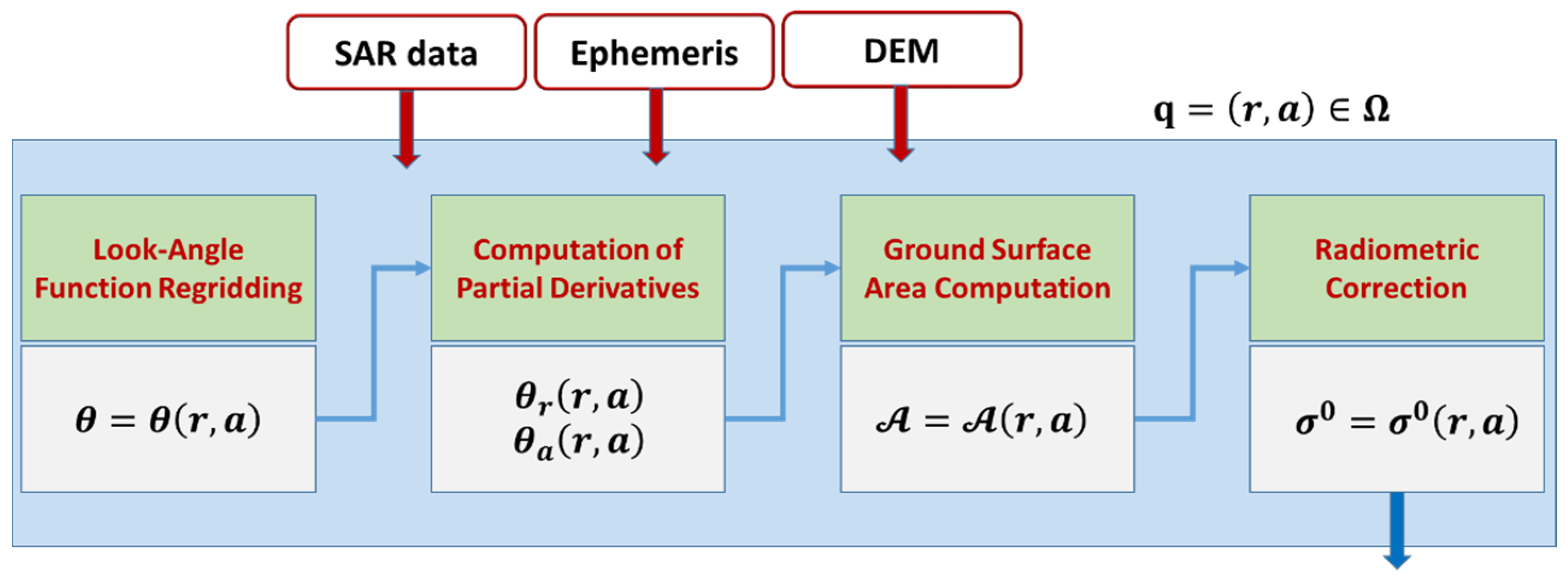
4.1. Implementation of a Prototype for SAOCOM Images Processing

In order to apply the adopted calibration method to SAOCOM data, we developed a dedicated numerical implementation, and the resulting prototype was used in this study. Specifically, the specialized prototype was obtained by suitably adapting the original processing kernel for processing SAOCOM data [10,17]. For such purpose, we focused on (1) the data ingestion operation, with the preprocessing subsystem implementing the construction of the dataset of a prescribed meta-sensor, (2) the suitable updating of the data management operation, and (3) the testing and validation of the implemented prototype. We highlight that, in the SAOCOM case, all the metadata associated with the SAR image were provided in XML files, whereas binary files contained the SAR image.
Concerning absolute radiometric calibration, it is worth noting that the SAOCOM data were obtained in a form in which the calibration constant had already been applied, as derived by relying on the reference targets at the calibration site [15].

4.2. Study Area and Dataset

The study area is located in the Calabria region (the southernmost region of the Italian Peninsula), which includes both vegetated areas with significant topographic variations and urban areas (see Figure 5).
In particular, more than 90% of the region is characterized by mountains and hills, including the Sila Mountains, the plateau of Aspromonte, and the massif of Pollino.
The Calabrian region is located between the Ionian Sea and the Tyrrhenian Sea and has almost 800 km of coastline. The reason for selecting this region is twofold. It is characterized by a complex topography. Moreover, it is also particularly important for applications, being characterized by extreme hydrological events, including floods and landslides [28], and is one of the most seismically active regions in the Mediterranean [29]. The experimental investigation was performed considering a dual-polarization SAOCOM-1A (SAO1A) L-band SAR data acquired over the selected mountainous area.
The SLC (single-look complex) data were acquired in the stripmap acquisition mode on 8 October 2021. Figure 5 shows the SAR data footprint superimposed on the Google Earth map of the study area. The nominal resolution was 4.99 m in the azimuth direction, and 5.42 m in the range direction. The main parameters of the selected SAR data are summarized in Table 1.
The ground shape description used in this investigation was derived from the digital elevation model (DEM) of the space shuttle radar topography mission (SRTM) with 1 arc-second spacing (i.e., the sampling step of the data product was approximately 30 m at the equator). The world geodetic system (WGS84) datum was used in this study [30].
Accordingly, we preliminarily converted SRTM DEM heights from EGM96 geoid to the WGS84 ellipsoid.
As in common practice, a suitable upsampling was applied to the original SRTM data, thus obtaining a DEM with pixel spacing comparable with the SAR data spacing. This operation was performed only for the benefit of the numerical implementation of the inherent mapping [10], and it did not affect the original data resolution.
It should be noted that the higher the geometric resolution of the original DEM is, the more accurate the estimation of the scattering area is. Nonetheless, high-resolution DEMs might be hard to obtain on a global scale, while SRTM-collected data cover about 80 percent of all the land on Earth.
Regarding the numerical parameters of the computation, we underline that the SAR system’s sampling parameters (see Table 1) determine the pixel size (azimuth × slant-range) in the image domain and hence the pixel size of the simulated radiometric distortion in the same domain. It should be noted that in the present SAOCOM case, the pixel size of the image (4.99 m × 3.74 m) was larger than that of the Cosmo-Skymed sensor (2.33 m × 1.33 m) used in [10]. Based on this parameter, DEM upsampling was arranged accordingly. On the other hand, we highlight that the image size (26,749 × 7935) was the main factor (Table 1) affecting the overall computational cost of the implemented procedure.

4.3. Experimental Results

In this study, the calibration method presented in Section 2 was applied for the radiometric calibration of SAOCOM data, thus specifically demonstrating its usefulness and relevance for sensors operating in the L-band as well.
The topographic pattern of the investigated area is illustrated in Figure 6. The SAR image footprint covered an area ranging between 39.0871°–40.0740° N and 15.8934°–16.8712° E.
The mean altitude of the investigated area was approximately 494 m, ranging roughly from 32 m to 2300 m. As far as scenarios with remarkable topographic reliefs are concerned, the associated large modulations severely affect the SLC image amplitude, and they can easily be compensated for in the imaging domain by specifically using the implemented solution.
In accordance with the method introduced in Section 2, the distortion simulation strategy relied on the computation of the magnitude of the gradient of the look-angle function evaluated in the image domain. First, the pattern of radiometric distortion was simulated, according to the processing scheme described in Figure 2, and then it was used to rectify the SLC image, as detailed in the following.
The look-angle function was evaluated over the swath, ranging from 30.4° to 34.5° (see Figure 7). This uniquely captures the signature of the topography as viewed by the SAR sensor; thus, it concisely conveys all the information needed for computing the correctable SAR radiometric distortions induced by topography. This is a straightforward but central observation, as it renders many complicated calculations unnecessary.
Secondly, according to the processing scheme in Figure 2, the (range-weighted) partial derivative of the look-angle function along the range and azimuth directions in the image space were computed separately.
The magnitude of the (range-weighted) partial derivative of the look-angle function, along the range and azimuth directions, are represented in Figure 8 and Figure 9, respectively.
It is clear that a steeper local look-angle function slope along the range and azimuth directions caused larger distortion. According to (4)–(6), both terms associated with the look-angle partial derivatives contribute to different degrees in determining the amount of local distortion.
As can be seen from Figure 8, the derivative of the look-angle function along the slant-range (radial) direction, θ r became negligible as the grazing condition was reached [10]. Figure 9 shows the contribution to the overall radiometric distortion term associated with the magnitude of the partial derivative of the look-angle function along the azimuth direction, θ a , which became particularly significant over some steep regions (depicted in red in Figure 9). On the other hand, the quantity θ a is negligible on the flatlands and vanishes over the sea (flat) area, as can be easily recognized in Figure 9. It should be noted that the depicted quantity is relevant to the partial derivative regardless of its sign, although the look-angle function might increase or decrease along the azimuth direction.
The local incidence angle (LIA) can be also computed according to the formalism in [10], and therefore the function χ l = χ l r , a evaluated in the image space is depicted in the range [0, 90°] in Figure 10.
The simulation of the radiometric distortion pattern was directly performed in terms of a scalar function, i.e., the magnitude of the gradient of the look-angle function.
As seen in the processing scheme in Figure 2, the overall radiometric distortion pattern was finally computed by using (2)–(3), and the obtained result is provided (in a suitable logarithmic scale) according to a suitable color-coded representation in Figure 11.
As can be recognized in Figure 11, the larger radiometric distortions (in red) correspond to higher values of the look-angle partial derivatives (see Figure 8 and Figure 9).
Conversely, at near grazing incidence (i.e., LIA approaching 90°), the look-angle partial derivatives are negligible, and accordingly, the associated local radiometric distortion becomes unitary (in linear scale). Note that over flat regions, the radiometric distortion, however, is not unitary (i.e., it is not zero on a logarithmic scale) and depends on the look-angle as well, in accordance with (13).
An important advantage of the adopted SAR image calibration method resides in its underlying compact analytical formulation, which essentially requires the calculation of the partial derivatives of the look-angle function defined in the image space.
The backscattering coefficient σ ~ V V 0 (in dB) obtained from the entire SLC image acquired in VV polarization is depicted in Figure 12.
We specifically used the symbol σ ~ V V 0 to emphasize that the (pseudo)backscattering coefficient was obtained without applying the compensation of topography-induced radiometric distortions. As can be clearly recognized through a visual inspection of Figure 11 and Figure 12, the simulated distortion pattern in Figure 11 follows the same structure of the σ ~ V V 0 image affected by topography-induced distortions (Figure 12).
Finally, the computed distortion pattern was applied to rectify the imaging distortions induced by the topography (also see Figure 2), and the resulting (calibrated) backscattering coefficient σ V V 0 is presented in Figure 13. A visual inspection of Figure 12 and Figure 13 indicates that the local radiometric distortions were largely rectified.
To better elucidate the obtained results, we now focus on two selected subregions, denoted as R1 and R2, both indicated in Figure 12 (with a box with perimeter lines dotted in red).
In particular, the backscattering coefficients obtained for the selected subregion R1, before and after the radiometric compensation are shown in Figure 14a,b, respectively. The effect of the applied compensation is supported by a visual inspection of Figure 14.
In order to understand the effect of the radiometric compensation in Figure 14 quantitatively, we depict the relevant backscattering coefficient (in dB) versus the local incidence angle (in degrees) obtained before (Figure 15a) and after (Figure 15b) the topography-induced radiometric distortion compensation was applied.
We underline that, in the scatterplots in Figure 15, the number of occurrences (in %) normalized to the total number of image pixels (4,000,000 samples) is taken into account, with the color bars representing the different colors assigned to different classes.
From an inspection of the scatterplots in Figure 15, the effect of the applied radiometric compensation on the overall dependency of the backscattering coefficient on the local incident angle is evident. For both cases (Figure 15a,b), robust linear regression was also estimated by using a least absolute deviation (or L1-norm regression) technique, which minimizes the L1-norm of the residuals. Specifically, in Figure 15a,b, we also depict the estimated regression lines (solid black line), with y = 8.07 0.07 x and y = 12.44 0.02 x , respectively. Remarkably, we found that the slope (dB/degree) value reduced from 0.07 (uncompensated topography-induced radiometric distortions) to 0.02 after radiometric calibration.
Similarly, the results obtained for the selected subregion R2 (see Figure 12), which had the same dimensions as R1, before and after the radiometric distortion compensation was applied are depicted in Figure 16a,b, respectively. Likewise, a representation in terms of scatterplots is given in Figure 17: in particular, the estimated regression lines for Figure 17a,b are y = 7.63 0.097 x and y = 11.64 0.051 x , respectively.
As can be seen from Figure 14a and Figure 15a (or Figure 16a and Figure 17a), the distortions associated with the imaging of the underlying topography caused by the effect of scattering ground area indicated important alterations in the radiometric information of the SAR image, which tend to dominate for small local incident angles. Therefore, the applied calibration operation significantly reduced the trend of decreasing backscattering with increasing local incidence angle (see Figure 14b and Figure 15b, or Figure 16b and Figure 17b). It should be noted that the backscattering cross-section per unit area on the ground, derived by removing the artifacts caused by radiometric imaging distortions, remains a function of the local incident angle, i.e., σ 0 = σ 0 ( χ l ) , in accordance with the electromagnetic scattering theory [19,20,21,22].

4.4. Remarks on the Backscattering Angular Dependence

It is worth noting that some topographic effects (see, for instance, Figure 13, Figure 14b, or Figure 16b) persisted in the sigma-naught image (compensated for topography-induced radiometric distortions). This is because backscattering coefficients indeed are an intrinsic function of the local incidence angle, which in turn depends on the local topography, as noted previously.
As a matter of fact, the backscattering dependence on the local incidence angle χ l was initially described according to Lambert’s law, by resorting to simple cosine model-based expression σ 0 = σ m 0 cos χ l n , where σ m 0 is the (maximum) backscattering value independent of the incidence angle effect, and n is the power index characterizing surface roughness [31,32]. Few surfaces behave as truly Lambertian surfaces in nature, and accordingly, the related empirical or semiempirical models exhibit limited validity. Nonetheless, backscattering coefficients are related to several parameters describing physical (geometric and electromagnetic) characteristics of the distributed target, including local incidence angle, soil moisture, surface roughness, and dielectric constant.
In the general case, the observed scene can be assimilated to an N-layered structure; thus, its backscattering coefficients might be parametrically expressed as follows [33,34]:
σ p q 0 = f χ l , λ , ε , t , s , l
where χ l is the local incidence angle, λ is the operative wavelength, and p and q are the polarizations of the incident and scattered waves, respectively. In addition, ε = [ ε 1 , ε 2 , . . . , ε N ] is the vector of the complex dielectric constant of the different layers, t = [ t 1 , t 2 . . , t N ] is the vector of the thickness of the different layers, s = [ s 1 , s 2 . . , s N ] is the vector of the rough interface root mean square height, and l = [ l 1 , l 2 . . , l N ] is the vector of the rough interface correlation length. Resorting to a layered description turns out particularly appropriate insofar as the L-band wave-penetration capabilities are more prominent with respect to higher frequency (C or X) bands.
It is then clear that the radiometric calibration operation and model-based application have to be adopted in an integrated way to proceed with a meaningful quantitative analysis (surface properties retrieval) and interpretation of SAR data, especially when the joint analysis of the heterogeneous multichannel (i.e., multisensor or multiorbit) SAR observations is considered. In this circumstance, the backscattering coefficients, obtained by suitably compensating the SAR images for different radiometric distortions, refer to different local incident angles, and therefore their meaningful exploitation requires the use of suitable parametric scattering models.

5. Conclusions

In this paper, the compensation of topography-induced radiometric distortions was investigated using SAOCOM images. The adopted calibration method, which has been recently developed, relies on an analytical formulation derived from the rigorous framework of differential geometry [10].
This manuscript conveys novelties in several respects, with both theoretical and applicative relevance:
(1)
From a theoretical perspective, we provided an original interpretation of the analytical expressions of the formulation in [10], thus providing further insights into the area-stretching-based formalism;
(2)
The numerical implementation of the method was specialized to process SAOCOM data, with special emphasis on data ingestion operation, meta-sensor data structure assembly, and related management operations. A software prototype was conceived to systematically process the radar data acquired by SAOCOM, and the tested prototype was subsequently used in this study;
(3)
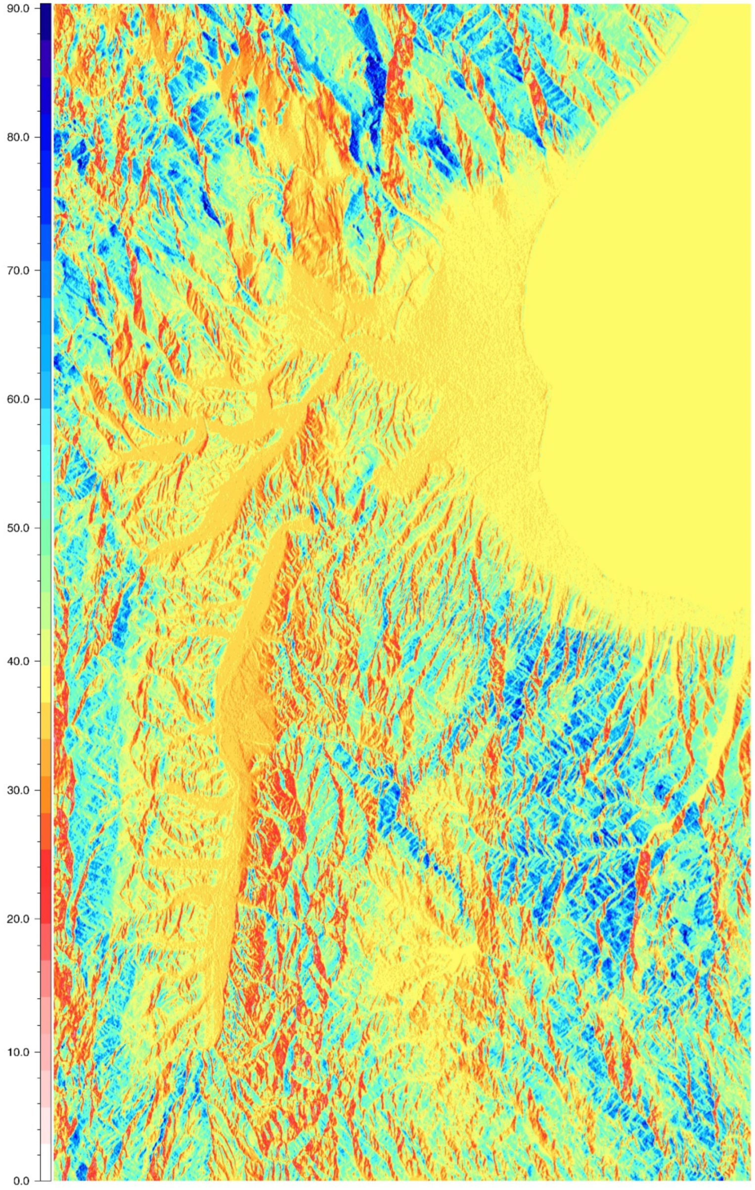
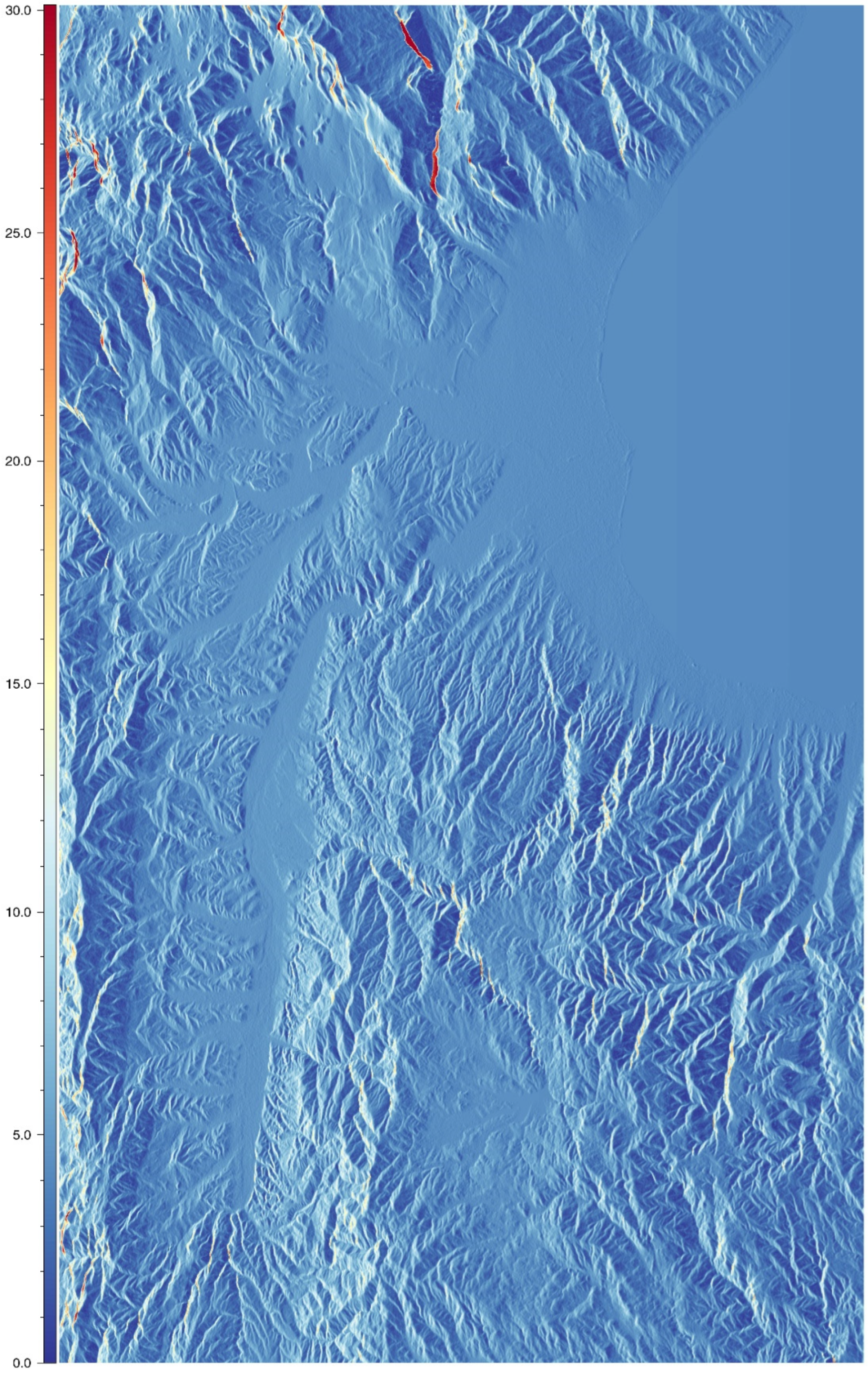
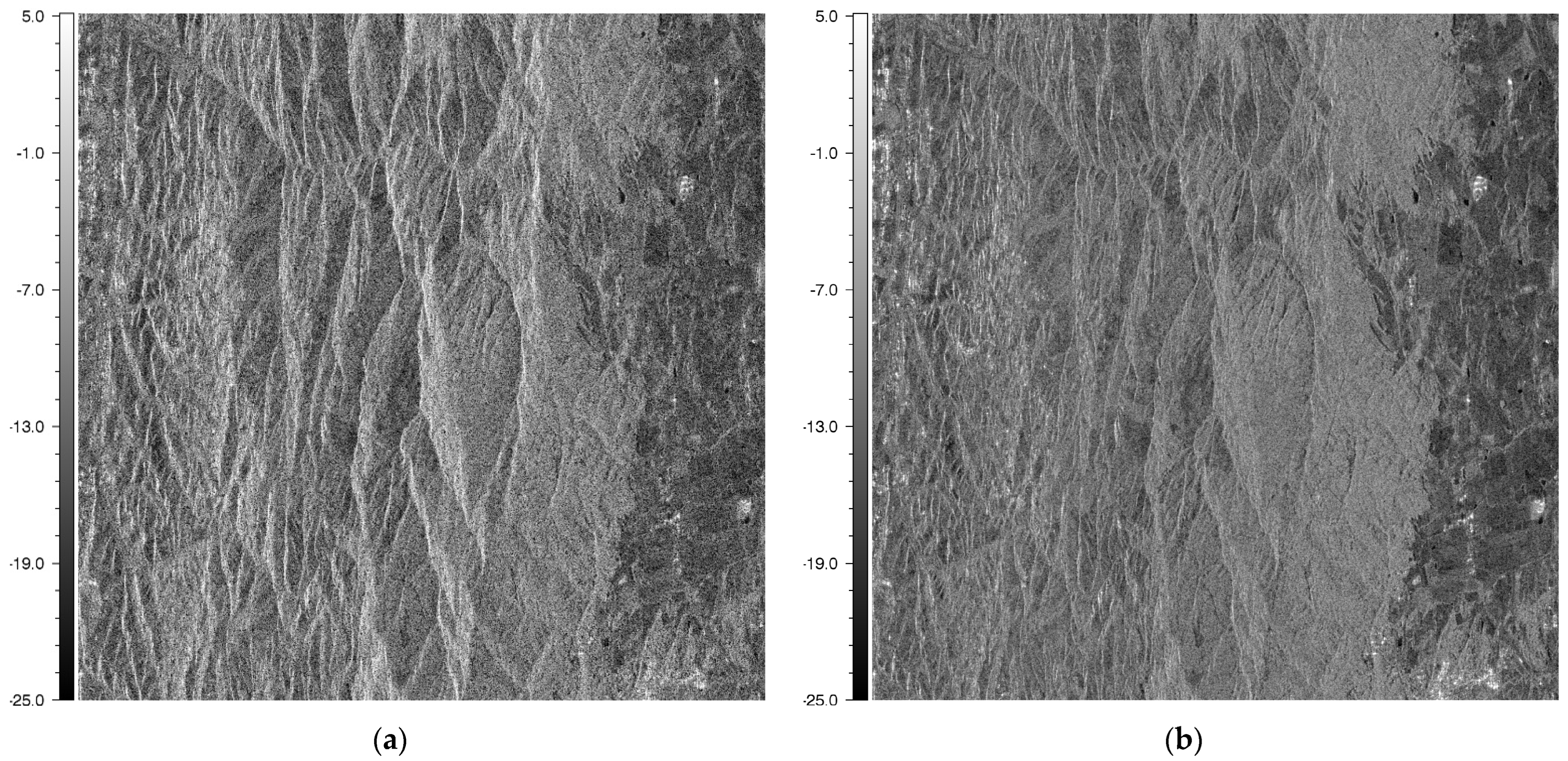
The experimental investigation was conducted by using the prototype processor for SAOCOM image calibration and was supported with illustrations and critical discussion of the obtained quantitative results, thus elucidating the effectiveness of the adopted methodology. Specifically, the experimental results were obtained by using SAOCOM data acquired over a mountainous region in the southern part of Italy;
(4)
The developed prototype provides a useful tool potentially exploitable in all remote sensing applications relying on the SAR amplitude information, thus enabling the operational use of the adopted differential-geometry-based SAR radiometric calibration method in large-scale SAOCOM data processing.
Some considerations on the comparison of the adopted method with respect to other SAR calibration algorithms are in order. Indeed, comparing the results obtained with the diverse existing radiometric calibration approaches [2,3,4,5,6,7,8,9] is not a simple task, insofar as they may include different assumptions, parameters, and specific algorithmic implementations, as noted, for instance, in [35]. Consequently, a consistent and meaningful assessment might be generally difficult to obtain with a superficial direct comparison. Moreover, this difficulty is exacerbated by the lack of SAR-independent reference results, with respect to which none of the existing approaches have been validated hitherto. Nonetheless, a theoretical comparison of the method adopted in this paper with respect to the method based on the projected local incidence angle (or projection cosine approach) [3] is provided in [10], thus demonstrating the local consistency of the two methods.
A fair comparison between different calibration methods would require the availability of an appropriate “ground-truth” reference reflectivity, which is, however, not available for actual images. In fact, working towards the development of such a benchmarking tool, possibly based on system-level simulation, is certainly interesting and an object of current research by the authors.
In future work, we also plan to realize an efficient implementation of the adopted processing strategy for SAR image calibration, which is indeed amenable to be inherently parallelized by employing shared-memory architectures and multithreading [36] or advances in GPU technology [37]. The relevant parallel prototype will boost its operational use in large-scale SAR data processing. In addition, quad-pol data processing will be addressed in future investigations [38].
Another perspective involves an extension of the proposed method to the case of heterogeneous multichannel (i.e., multisensor or multiorbit) SAR observations, in which dissimilar viewing geometries might be prone to misleading interpretation. As a result, the joint use of the information from heterogeneous multichannel SAR observations is not trivial, and therefore the full exploitation of consistently integrated SAR images affected by different distortions still presents unexplored aspects in the domain of remote sensing.

Author Contributions

Conceptualization, P.I. and G.D.M.; methodology, P.I. and G.D.M.; software, P.I.; validation, P.I. and G.D.M.; formal analysis, P.I.; writing—original draft preparation, P.I.; writing—review and editing, P.I. and G.D.M. All authors have read and agreed to the published version of the manuscript.

Funding

This work was partially supported by the European Union under the Italian National Recovery and Resilience Plan (NRRP) of NextGenerationEU, partnership on “Telecommunications of the Future” (PE00000001—program “RESTART”).

Data Availability Statement

Not applicable.

Acknowledgments

The SAOCOM data used for this work were kindly made available through the MEFISTO project funded by ASI (Italia Space Agency).

Conflicts of Interest

The authors declare no conflict of interest.

References

  1. Freeman, A. SAR calibration: An overview. IEEE Trans. Geosci. Remote Sens. 1992, 30, 1107–1121. [Google Scholar] [CrossRef]
  2. Van Zyl, J.; Chapman, B.; Dubois, P.; Shi, J. The effect of topography on SAR calibration. IEEE Trans. Geosci. Remote Sens. 1993, 31, 1036–1043. [Google Scholar] [CrossRef]
  3. Ulander, L. Radiometric slope correction of synthetic-aperture radar images. IEEE Trans. Geosci. Remote Sens. 1996, 34, 1115–1122. [Google Scholar] [CrossRef]
  4. Shimada, M. Ortho-Rectification and Slope Correction of SAR Data Using DEM and Its Accuracy Evaluation. IEEE J. Sel. Top. Appl. Earth Obs. Remote Sens. 2010, 3, 657–671. [Google Scholar] [CrossRef]
  5. Löw, A.; Mauser, W. Generation of geometrically and radiometrically terrain corrected SAR image products. Remote Sens. Environ. 2007, 106, 337–349. [Google Scholar] [CrossRef]
  6. Gelautz, M.; Frick, H.; Raggam, J.; Burgstaller, J.; Leberl, F. SAR image simulation and analysis of alpine terrain. ISPRS J. Photogramm. Remote Sens. 1998, 53, 17–38. [Google Scholar] [CrossRef]
  7. Simard, M.; Riel, B.V.; Denbina, M.; Hensley, S. Radiometric Correction of Airborne Radar Images Over Forested Terrain With Topography. IEEE Trans. Geosci. Remote Sens. 2016, 54, 4488–4500. [Google Scholar] [CrossRef]
  8. Frey, O.; Santoro, M.; Werner, C.L.; Wegmuller, U. DEM-based SAR pixel-area estimation for enhanced geocoding refinement and topographic normalization. IEEE Geosci. Remote Sens. Lett. 2013, 10, 48–52. [Google Scholar] [CrossRef]
  9. Holecz, F.; Pasquali, P.; Moreira, J.; Nuesch, D. Rigorous radiometric calibration of airborne AeS-1 InSAR data. In Proceedings of the IGARSS’98. Sensing and Managing the Environment. 1998 IEEE International Geoscience and Remote Sensing. Symposium Pro-ceedings, Seattle, WA, USA, 6–10 July 1998; Volume 5, pp. 2442–2444. [Google Scholar] [CrossRef]
  10. Imperatore, P. SAR Imaging Distortions Induced by Topography: A Compact Analytical Formulation for Radiometric Calibration. Remote Sens. 2021, 13, 3318. [Google Scholar] [CrossRef]
  11. Small, D. Flattening Gamma: Radiometric Terrain Correction for SAR Imagery. IEEE Trans. Geosci. Remote Sens. 2011, 49, 3081–3093. [Google Scholar] [CrossRef]
  12. Imperatore, P.; Azar, R.; Calo, F.; Stroppiana, D.; Brivio, P.A.; Lanari, R.; Pepe, A. Effect of the Vegetation Fire on Backscattering: An Investigation Based on Sentinel-1 Observations. IEEE J. Sel. Top. Appl. Earth Obs. Remote Sens. 2017, 10, 4478–4492. [Google Scholar] [CrossRef]
  13. Anconitano, G.; Acuna, M.A.; Guerriero, L.; Pierdicca, N. Analysis of Multi-Frequency SAR Data for Evaluating Their Sensitivity to Soil Moisture Over an Agricultural Area in Argentina. In Proceedings of the IGARSS 2022—2022 IEEE International Geoscience and Remote Sensing Symposium, Kuala Lumpur, Malaysia, 17–22 July 2022; pp. 5716–5719. [Google Scholar] [CrossRef]
  14. Machado, F.; Solorza, R. Feasibility of the inversion of electromagnetic models to estimate soil salinity using SAOCOM data. In Proceedings of the 2020 IEEE Congreso Bienal de Argentina (ARGENCON), Resistencia, Argentina, 1–4 December 2020; pp. 1–8. [Google Scholar] [CrossRef]
  15. Azcueta, M.; Gonzalez, J.P.C.; Zajc, T.; Ferreyra, J.; Thibeault, M. External Calibration Results of the SAOCOM-1A Commissioning Phase. IEEE Trans. Geosci. Remote Sens. 2022, 60, 1–8. [Google Scholar] [CrossRef]
  16. Fioretti, L.; Giudici, D.; Guccione, P.; Recchia, A.; Steinisch, M. SAOCOM-1B Independent Commissioning Phase Results. In Proceedings of the 2021 IEEE International Geoscience and Remote Sensing Symposium IGARSS, Brussels, Belgium, 11–16 July 2021; pp. 1757–1760. [Google Scholar] [CrossRef]
  17. Imperatore, P.; Lanari, R.; Pepe, A. Gical: Geo-Morphometric Inverse Cylindrical Method for Radiometric Calibration of Sar Images. In Proceedings of the IEEE International Geoscience and Remote Sensing Symposium, IGARSS 2018, Valencia, Spain, 23–27 July 2018. [Google Scholar] [CrossRef]
  18. do Carmo, P.M. Differential Geometry of Curves and Surfaces; Prentice-Hall: Englewood Cliffs, NJ, USA, 1976. [Google Scholar]
  19. Ulaby, F.T.; Moore, R.K.; Fung, A.K. Microwave Remote Sensing: Active and Passive. Volume 2-Radar Remote Sensing and Surface Scattering and Emission Theory; Addison-Wesley: Boston, MA, USA, 1982. [Google Scholar]
  20. Ulaby, F.T.; Moore, R.K.; Fung, A.K. Microwave Remote Sensing: Active and Passive—Volume Scattering and Emission Theory, Advanced Systems and Applications; Artech House, Inc.: Dedham, MA, USA, 1986; Volume III. [Google Scholar]
  21. Tsang, L.; Kong, J.A.; Shin, R.T. Theory of Microwave Remote Sensing; Wiley: New York, NY, USA, 1985. [Google Scholar]
  22. Ishimaru, A. Wave Propagation and Scattering in Random Media; Academic Press: New York, NY, USA, 1993. [Google Scholar]
  23. Raney, R.K.; Freeman, T.; Hawkins, R.W.; Bamler, R. A plea for radar brightness. In Proceedings of the IGARSS’94-1994 IEEE International Geoscience and Remote Sensing Symposium, Pasadena, CA, USA, 8–12 August 1994. [Google Scholar]
  24. Kropatsch, W.; Strobl, D. The generation of SAR layover and shadow maps from digital elevation models. IEEE Trans. Geosci. Remote Sens. 1990, 28, 98–107. [Google Scholar] [CrossRef]
  25. Schreier, G. (Ed.) Geometrical properties of SAR images. In SAR Geocoding: Data and Systems; Wichmann: Karlsruhe, Germany, 1993; pp. 103–134. [Google Scholar]
  26. Curlander, J. Location of space borne SAR imagery. IEEE Trans. Geosci. Remote Sens. 1982, GRS-20, 359–364. [Google Scholar] [CrossRef]
  27. Curlander, J.C. Utilization of Spaceborne SAR Data for Mapping. IEEE Trans. Geosci. Remote Sens. 1984, GE-22, 106–112. [Google Scholar] [CrossRef]
  28. Reale, D.; Verde, S.; Calo, F.; Imperatore, P.; Pauciullo, A.; Pepe, A.; Zamparelli, V.; Sansosti, E.; Fornaro, G. Multipass InSAR with Multiple Bands: Application to Landslides Mapping and Monitoring. In Proceedings of the IGARSS 2022—2022 IEEE International Geoscience and Remote Sensing Symposium, Kuala Lumpur, Malaysia, 17–22 July 2022; pp. 4510–4513. [Google Scholar] [CrossRef]
  29. Pavano, F.; Gallen, S.F. A Geomorphic Examination of the Calabrian Forearc Translation. Tectonics 2021, 40, e2020TC006692. [Google Scholar] [CrossRef]
  30. Iliffe, J. Datums and Map Projections for Remote Sensing, GIS, and Surveying; CRC Press: Boca Raton, FL, USA, 2000. [Google Scholar]
  31. Menges, C.H.; Van Zyl, J.J.; Hill, G.J.E.; Ahmad, W. A procedure for the correction of the effect of variation in incidence angle on AIRSAR data. Int. J. Remote Sens. 2001, 22, 829–841. [Google Scholar] [CrossRef]
  32. Ulaby, F.T.; Moore, R.K.; Fung, A.K. Microwave Remote Sensing: Active and Passive; Addison-Wesley: Reading, MA, USA, 1981. [Google Scholar]
  33. Imperatore, P.; Iodice, A.; Riccio, D. Electromagnetic Wave Scattering from Layered Structures with an Arbitrary Number of Rough Interfaces. IEEE Trans. Geosci. Remote Sens. 2009, 47, 1056–1072. [Google Scholar] [CrossRef]
  34. Imperatore, P.; Iodice, A.; Pastorino, M.; Pinel, N. Modelling Scattering of Electromagnetic Waves in Layered Media: An Up-to-Date Perspective. Int. J. Antennas Propag. 2017, 2017, 7513239. [Google Scholar] [CrossRef] [Green Version]
  35. Truckenbrodt, J.; Freemantle, T.; Williams, C.; Jones, T.; Small, D.; Dubois, C.; Thiel, C.; Rossi, C.; Syriou, A.; Giuliani, G. Towards Sentinel-1 SAR Analysis-Ready Data: A Best Practices Assessment on Preparing Backscatter Data for the Cube. Data 2019, 4, 93. [Google Scholar] [CrossRef] [Green Version]
  36. Imperatore, P.; Sansosti, E. Multithreading Based Parallel Processing for Image Geometric Coregistration in SAR Interferometry. Remote Sens. 2021, 13, 1963. [Google Scholar] [CrossRef]
  37. Romano, D.; Mele, V.; LaPegna, M. The Challenge of Onboard SAR Processing: A GPU Opportunity. In Computational Science—ICCS 2020. ICCS 2020. Lecture Notes in Computer Science; Springer: Cham, Switzerland, 2020; Volume 12139. [Google Scholar] [CrossRef]
  38. Imperatore, P.; Pepe, A.; Lanari, R. Polarimetric Sar Distortions Induced by Topography: An Analytical Formulation for Compensation in the Imaging Domain. In Proceedings of the International Geoscience and Remote Sensing Symposium, IGARSS 2018, Valencia, Spain, 23–27 July 2018. [Google Scholar]
Figure 1. Schematic 3D representation of an arbitrarily orientated scattering surface element on the ground Φ = φ ( Ω ) , which is associated with a prescribed cell Ω in the image space. The cylindrical coordinate system is also shown.
Remotesensing 15 01286 g001
Figure 2. The image-domain processing scheme.
Remotesensing 15 01286 g002
Figure 3. Interpretative scheme for the reference azimuth-invariant topography elevation case: r is the increment along the slant-range coordinate, θ is the corresponding increment of the look-angle function, and r g is the associated ground-range increment.
Remotesensing 15 01286 g003
Figure 4. Interpretative scheme for the reference flat-Earth case: r is the increment along the slant-range coordinate, θ is the corresponding increment of the look-angle function, and r g is the associated ground-range increment.
Remotesensing 15 01286 g004
Figure 5. SAOCOM-1A data footprint is shown superimposed on the Google Earth map of the study area in southern Italy.
Remotesensing 15 01286 g005
Figure 6. Elevation (m) of the DEM.
Remotesensing 15 01286 g006
Figure 7. Look-angle function (LAF) (degree): θ = θ r , a . The range direction is from left to right; the azimuth direction is from bottom to top.
Remotesensing 15 01286 g007
Figure 8. Magnitude (dB) of the (range-weighted) partial derivative of the look-angle function along the range direction r θ r .
Remotesensing 15 01286 g008
Figure 9. Magnitude (dB) of the (range-weighted) partial derivative of the look-angle function along the azimuth direction r θ a .
Remotesensing 15 01286 g009
Figure 10. Local incidence angle (LIA) (degree): χ l = χ l r , a .
Remotesensing 15 01286 g010
Figure 11. Simulated radiometric distortion (dB) image associated with the ground surface area.
Remotesensing 15 01286 g011
Figure 12. Copolarized backscattering coefficient σ ~ V V 0 (dB) obtained from the SLC image without compensation of topography-induced radiometric distortions. Two selected subregions are indicated with two boxes with perimeter lines dotted in red.
Remotesensing 15 01286 g012
Figure 13. Copolarized backscattering coefficient σ V V 0 (dB) obtained from the SLC image by applying the compensation of topography-induced radiometric distortions.
Remotesensing 15 01286 g013
Figure 14. Backscattering coefficient (dB) of the selected subregion R1: (a) σ ~ V V 0 , without topography-induced radiometric distortion compensation; (b) σ V V 0 , including topography-induced radiometric distortion compensation.
Remotesensing 15 01286 g014
Figure 15. Backscattering coefficient (dB) vs. local incidence angle (degree) for the selected subregion R1: (a) σ ~ V V 0 , without topography-induced radiometric distortion compensation; (b) σ V V 0 , including topography-induced radiometric distortion compensation. The black lines represent robust linear regressions.
Remotesensing 15 01286 g015
Figure 16. Backscattering coefficient (dB) of the selected subregion R2: (a) σ ~ V V 0 , without topography-induced radiometric distortion compensation; (b) σ V V 0 , including topography-induced radiometric distortion compensation.
Remotesensing 15 01286 g016
Figure 17. Backscattering coefficient (dB) vs. local incidence angle (degree) for the selected subregion R2: (a) σ ~ V V 0 , without topography-induced radiometric distortion compensation; (b) σ V V 0 , including topography-induced radiometric distortion compensation. The black lines represent robust linear regressions.
Remotesensing 15 01286 g017
Table 1. SAR dataset characteristics.
SAR PlatformSAO1A
Acquisition date8 October 2021
Observation directionRight looking
PolarizationVV + VH
Orbit directionAscending
Carrier frequency (GHz)1.275
Off-nadir angle (degree)32.2174
Sampling frequency (MHz)30.00
Chirp bandwidth (MHz)24.40
PRF (Hz)1857.00
Azimuth bandwidth (Hz)1229.94
Azimuth-pixel spacing (m)3.74
Range pixel spacing (m)5.00
Azimuth resolution (m)4.99
Range resolution (m)5.42
Azimuth lines26749
Range samples7935
First near(latitude (deg), longitude (deg))(39.087114, 16.105089)
First far(39.967124, 15.893462)
Last near(40.074031, 16.669855)
Last far(39.193983, 16.871278)
Disclaimer/Publisher’s Note: The statements, opinions and data contained in all publications are solely those of the individual author(s) and contributor(s) and not of MDPI and/or the editor(s). MDPI and/or the editor(s) disclaim responsibility for any injury to people or property resulting from any ideas, methods, instructions or products referred to in the content.

