Increasing Accuracy of the Soil-Agricultural Map by Sentinel-2 Images Analysis—Case Study of Maize Cultivation under Drought Conditions

Abstract

The properties of soil constitute one of the most important features of the environment that determine the potential for food production in a given region. Knowledge of the soil texture and agroclimate allows for the proper selection of species and agrotechnics in plant production. However, in contrast to the agroclimate, the soil may show a large spatial variation of physical and chemical characteristics within the plot. In regions where the soil diversity is so high that the available soil maps are not sufficient, the only method that allows for precise mapping of the soil mosaic is remote sensing. This paper presents the concepts of using Sentinel-2 multispectral satellite images to detail the available soil-agriculture map at a scale of 1:25,000. In the presented work, the following research hypothesis has been formulated: spatial and temporal analysis of high-resolution satellite images can be used to improve the quality of a large-scale archival soil-agriculture map. It is possible due to the spatial differentiation of the spectral reflection from the field (canopy), which is influenced by soil conditions—especially the differentiation of physical properties (granulometric composition) in soil profiles which determine the possibility of water retention during drought conditions. The research carried out as a case study of maize remote sensing confirmed the hypothesis. It was based on the selection of the most appropriate term (maize development period: BBCH 79, 6-decade drought index: CBW = −206 mm) and the vegetation index (NDVI). This made it possible to make the scale of the map 10 times more detailed. The obtained results are the first step in developing a general model (based on remote sensing) for detailing the soil-agriculture map for Poland, which will significantly improve the accuracy of the drought monitoring system developed by the Institute of Soil Science and Plant Cultivation (Poland).

1. Introduction

The properties of soil, the suitability for the cultivation of particular crops and the agroclimate are the most important features of the environment that determine the potential for food production in a given region. These factors are usually interdependent, as weather patterns have a very strong impact on soil properties, and an optimal pattern is correlated with high yields. However, the variability of soil conditions is also influenced by other factors, such as the topography, type of vegetation cover, climatic situation in recent geological epochs, anthropopression, etc. These factors may lead to a large differentiation of the soil both in its surface layer and in the soil profile. Therefore, small-scale (overview) maps, such as FAO [1,2,3], USDA [4,5,6,7] or WRB [8,9], can only be used for illustrative purposes or for conducting trans-regional studies. In the case of regional surveys, more detailed soil maps are needed, the nomenclature of which is dedicated directly to the specificity of a given physio-geographical region or country. Due to this obvious soil variability, in recent decades national systems dedicated mainly to the needs of land valuation and management of this natural resource were developed independently. An example of this type of soil map is, e.g., the system of Polish soil valuation used in the research presented in this paper.

Poland has a long history and unique knowledge and experience in the field of agricultural and soil sciences. In 1816, in Marymont near Warsaw (capital city), the Agronomic Institute was established, which was later relocated to Puławy (the present location of the Institute of Soil Science and Plant Cultivation: IUNG-PIB), where in 1894 Vasily Dokuczajew founded the world’s first independent department of soil science [10]. The first attempts at detailed classification and mapping of Poland’s soils were made in the early 1950s. In the period of 1956–1967, the qualitative classification of soils covering the whole country was elaborated, which referred to the morphological features, some physical and chemical properties and the production potential of the soils cultivated for agricultural purposes. Furthermore, this work has helped to establish the background for the development of the land value tax system for the government, rural development plans for different regions, national cadaster of land and buildings and has provided valuable data for many scientific works in the field of agronomy [11,12]. The cartographic survey work was performed using a standardized and uniform method under defined procedures described in the guidelines [13].

The descriptive and mapping data gathered in this procedure were used by IUNG-PIB to develop another functional classification regarding the agricultural suitability of soils based on the ability to grow indicator and co-indicator crops [14,15]. Arable land was classified into fourteen complexes, and stable grasslands into three complexes. A more detailed description can be found in

Table A1. Part of the description of Polish soil classification system used for the soil map at a scale of 1:25,000.

Soil agricultural suitability complexes
Soil complexes of arable lands
1	Very good wheat soil complex
2	Good wheat soil complex
3	Defective wheat soil complex
4	Very good rye (wheat–rye) soil complex
5	Good rye soil complex
6	Weak rye soil complex
7	Very weak rye (rye–lupin) soil complex
8	Cereal–fodder strong soil complex (mainly for wheat)
9	Cereal–fodder weak soil complex (mainly for rye)
10	Mountain wheat soil complex
11	Mountain cereal soil complex
12	Mountain oat–potatoes soil complex
13	Mountain oat–fodder soils complex
14	Arable lands for grasslands
Soil complexes of permanent grasslands
1z	Good and very good grasslands (occasionally flooded)
2z	Medium quality grasslands (high situated, not flooded)
3z	Weak and very weak grasslands (peaty and post-peaty)
RN	Soils unsuitable for agriculture (which can be afforested)
Other elements of the map content
Ls	Forests
Tz	Built-up areas (with dense housing) and residential areas
W	Waters
WN	Waters wastelands
N	Agricultural wastelands
Soil types and subtypes
/no symbol/	Immature soils, rankers
A	Podzolic and pseudo-podzolic soils
B	Typical brown soils
Bw	Leached brown soils and acid brown soils
C	Typical chernozems (also called black soil)
Cz	Degraded chernozems and grey soils
D	Proper black earths
Dz	Degraded black earths and grey soils
G	Gley soils
E	Alluvial muck soils on peat subsoil and peat soils on alluvial subsoil, peat-mud soil
M	Peaty soils and mucky soils
T	Peat soils and peat-muck soils
F	Alluvial soils, fluviosoles
Fb	Brown alluvial soils
Fc	Chernozem alluvial soils
FG	Alluvial gley soils
R	Initial rendzinas
Rb	Brown rendzinas
Rc	Humous rendzinas (from black earth and grey earth)
d	Deluvial sediments
Soils texture groups and classes
Gravelly soils
żp	sandy gravels
żg	loamy gravels
Sandy soils
pl	loose sands
ps	weakly loamy sands
pgl	light loamy sands
pgm	strong loamy sands
Loamy soils
gl	light loams
gs	medium loams
gc	heavy loams
Silty soils
płz	typical silts
płi	clayey silts
l	loess
li	clayey loess
Clayey soils
ip	silty clays
i	clays
Symbol “p” added to soil texture means high silt content
Rendzinas
l	light rendzinas
s	medium rendzinas
c	heavy rendzinas
Alluvial soils
bl	very light alluvial soils
l	light alluvial soils
s	medium alluvial soils
c	heavy alluvial soils
Peat soils and alluvial muck soils on peat subsoil
n	fen peat
v	transition and highmoor peat
mt	alluvial muck soils on peat subsoil
tm	peat soils on alluvial subsoil.

(Appendix A). Appropriate crop species selection based on the soil complex is one of the basic conditions determining the yield level. The assignment process of crops to particular soil complexes was carried out using several criteria: soil properties, relief, climatic and water conditions, as well as potential agricultural purposes of the farmland. The results of this work were soil-agricultural maps for the whole country drawn at scales from very general 1:1,000,000, through 1:100,000 to 1:25,000, to the most detailed 1:5000, on which complexes, types and subtypes, families and textural groups to a depth of up to 150 cm were determined [16].

Based on the reclassification of the 1:25,000 scale digital map of soil agriculture, a soil drought vulnerability category map was developed. This map shows the four categories that are considered in the Agricultural Drought Monitoring System (ADMS) conducted by the official national system [17,18,19,20]. Such a detailed map has been successfully used since 2008 to assess the extent of agricultural drought in the basic administrative units of the country (NUTS-5). In 2020, the drought monitoring system was refined to assess yield losses due to water shortages in the scale of agricultural parcels. However, in many regions, a detailed assessment of crop losses caused by drought may require maps of a larger scale, due to the mosaic of soil on the scale of fields. In this case, the most efficient option is to use remote sensing. The research conducted so far proves that both aerial photos and satellite images allow for effective mapping of spatial variability of soil properties [21,22,23,24]. Contrary to direct in situ studies, remote sensing does not allow direct determination of physical or chemical properties, but gives an image that can be interpreted when analyzing the extent of soil complexes on a map [25,26,27]. Information on the diversity of soil on the scale of individual fields can be provided both by photos of the exposed soil as well as images of the diversity of vegetation indices in the canopy [28,29,30]. The Copernicus Program, run by the European Space Agency with the participation of the European Commission, provided wide possibilities of using satellite remote sensing data [31,32,33]. Public access to Sentinel-2 images [34], available since 2016, has opened the possibility of conducting high-resolution observations in time and space for most agricultural land parcels in Poland that meet the minimum size and shape criteria for this resolution [19,35,36].

The overview of the existing works on remote sensing in agriculture allows for the formulation of the following research hypothesis: spatial and temporal analysis of high-resolution satellite images can be a source used to improve the quality of large-scale archival soil maps. It is possible thanks to the spatial differentiation of the spectral reflection from the field (canopy), which is influenced by soil conditions—especially the differentiation of physical properties (granulometric composition) in soil profiles, which determines the possibility of water retention during drought conditions.

2. Materials and Methods

2.1. Study Area Location

The study area was located in the “Baborówko” Experimental Station (BES) (Figure 1), being a part of the IUNG-PIB. Baborówko is situated in the western part of Poland (central point 16°38.47′E, 52°35.29′N). Geographically, this region belongs to the province Central European Lowland; subprovince Southern Baltic Lake Districts; macroregion Greater Poland Lake District; mesoregion Poznań Lake District [37]. Due to this location, the region contains agricultural areas with high variability of soil characteristics. The mosaic which can be observed within the boundaries of small arable fields resulted from the geomorphological processes that took place in the past: there were at least three transgressions and regressions of the ice sheet [38,39]. The Wielkopolska region has a very long agricultural tradition of large holdings and intensive farming production. Already in the Middle Ages, there were large agricultural farms with intensive cereal cultivation. Although natural conditions in this area were not very favorable, farmers have been able to achieve high yields (significantly above the national average) [40] by proper management and good agronomic knowledge. The influence of the oceanic climate is visible in this area, represented by very mild winters with little or no snow cover; there are significant precipitation fluctuations, droughts occur quite often (in the period of 2011–2021 the hazard of strong agricultural drought occurred five times) and their distribution in time is rather unfavorable: dry springs and intensification of drought in summer (in July), long periods without precipitation interrupted by very rapid and heavy rainfall [41]. In addition, anthropogenic activity has significantly contributed to the worsening of water balance, i.e., river regulation, draining of swamps, deforestation, land melioration and creation of large arable fields caused the steppification of this area.

The abovementioned characteristic is also present in the pilot area. The complicated soil morphology (due to high soil heterogeneity) is mainly a result of the mentioned post-glacial geomorphological processes. On the fields, it can be observed that at very short distances (even for transects no longer than 10 m) the soil profile differs significantly—e.g., light soil (loose sand to a depth of 150 cm) can be found in the close neighborhood of medium soil with a denser granulometric composition, i.e., strong loamy sand underlain by light clay. Therefore, the following investigation has been undertaken regarding the possibility of detailing the existing soil map at a scale of 1:25,000 (map of soil drought vulnerability categories) with the use of high-resolution satellite images of Sentinel-2 taken during strong water stress, which can indirectly indicate soil heterogeneity by differentiating the greenness of plant canopy cover. For the analysis, there were selected fields with maize cultivation in 2020, with a total area of 100 ha (Figure 1).

For testing the assumed hypothesis, the year with the largest agricultural drought recorded by ADMS was selected, for which the Sentinel-2 imagery was available. Water deficit in the analyzed growing season for maize cultivation had a significant impact on plants, which caused the greatest crop losses on this farm in the last 5 years (2017—10.0 t × ha⁻¹, 2018—7.6 t × ha⁻¹, 2019—9.4 t × ha⁻¹, 2020—6.1 t × ha⁻¹, 2021—6.5 t × ha⁻¹).

2.2. Materials

For this research, the following were used: a soil-agricultural map and soil drought vulnerability category map describing the soil variability; ground data—meteorological data, observations of maize growth and development, and soil samples to validate the obtained results; satellite data—vegetation index maps (VI).

2.2.1. Soil-Agricultural Map and Soil Drought Vulnerability Category Map

Digital maps held in the IUNG-PIB repository were used, i.e., the soil-agricultural map at a scale of 1:25,000 and the soil drought vulnerability category map, which is used in ADMS. The drought vulnerability soil map is derived from the soil-agricultural map and was created by reclassifying soil contours with described granulometric composition across the soil profile (Figure 2A) into contours of four classes of drought vulnerability soils (Figure 2B). To do this, knowledge about the available water capacity of the different soil textures was used (

Table 1. Description of soil drought vulnerability categories.

Name	Description	Available Water Capacity (AWC)
category I	Highly sensitive to drought	<127.5 mm
category II	Sensitive to drought	127.5–169.9 mm
category III	Moderately sensitive to drought	170.0–202.5 mm
category IV	Slightly sensitive to drought	>202.5 mm

Source: [17,42].

, see also

Table A2. Parameters of available water capacity for plants in various granulometric soil grain [42].

Soil Textural Groups	Available Water Capacity (AWC) [mm]
loose sands (pl)	92
slightly loamy sands (ps)	117
weakly loamy sands (pgl)	138
strong loamy sands (pgm)	155
light loams (gl)	185
medium-heavy loams (gs)	205
heavy loams (gc)	240

in Appendix A). In other words, the basic factor that determines the belonging of a soil contour to a soil category is the granulometric composition and its differentiation in the soil profile.

These analyses were based on soil-agricultural map contours with an assigned drought vulnerability category for the study area. It should be noted that category IV was not found in the studied fields, this is the category that has the greatest capacity to retain water.

Map of soil vulnerability to drought categories is directly used in the Agricultural Drought Monitoring System, hence the decision on such a choice, in the event of positive verification of the working hypothesis, may contribute to the improvement of the estimation of yield losses to which this monitoring relates (operationally on a national scale). ADMS was described in detail by Szewczak et al. (2020) and Jedrejek et al. (2022) [19,43].

2.2.2. Ground Measurements and Observations

Meteorological Data

Meteorological data regarding precipitation, temperature, humidity, sunshine radiation and wind speed were obtained from a weather station located in the direct neighborhood of the BES sites. This station is part of the Agricultural Drought Monitoring System. Meteorological data were used for the calculation of daily evapotranspiration (according to the Penman–Monteith formula—FAO-56 Method) and climatic water balance [44,45].

Phenological Observations and Agrotechnical Treatments

Throughout the whole vegetation season, observations of maize growth and development on the “Biologische Bundesanstalt, Bundessortenamt und CHemische Industrie” (BBCH) scale were carried out [46].

The dates and types of agrotechnical treatments were recorded during the entire vegetation season, as well as the names and amounts of plant protection products and fertilizers used. All treatments were carried out on time and following the approved standards, no diseases, weeds or pests were observed. Soil analyses determining the content of other yield-forming components (pH in a 1-molar KCl solution; potassium and phosphorus—the Egner–Riehm method; magnesium—the complexometric method) are regularly performed, and fertilizers are selected based on these analyses. Maize was sown on 23–24 April 2020 and harvested on 16–18 October 2020. Nitrogen rate of 135 kg/ha (in two doses), potassium of 70 kg/ha and phosphorus of 40 kg/ha were applied during the analyzed season. Only one herbicide treatment was conducted in the second decade of May.

Soil Sampling

Thirty soil samples were collected, for which the granulometric composition (texture) was determined in the laboratory with the same reference standards (areometric method) and at the same depths (three depth levels: 0–30 cm, 30–50 cm; 50–100 cm) as specified on the soil map so that the calculated soil retention capacity would be comparable. The samples were collected for direct validation of the results of analysis. The sampling locations (Figure 1) were precisely determined by the differential GPS method.

2.2.3. Satellite Images and Vegetation Indices (VI) Maps

Sentinel-2 images were used as the remote sensing data. The choice was based on the following reasons:

• Public (free) access to data;
• Short revisit time (5 days);
• High spatial resolution (10, 20, 60 m) enabling observation of image diversity within the boundaries of agricultural plots;
• Imaging in the range of visible, red-edge and infrared radiation, which is important in research on the condition of vegetation.

In this study, a time series from 1 June 2020 to 30 September 2020 of cloud-free Sentinel-2A and Sentinel-2B images were analyzed, acquired as Level 2A products from the European Space Agency server [34,47]. All downloaded images were preprocessed by R package sen2r developed by the Institute of Remote Sensing of Environment (IREA) of the Italian National Research Council [48]. Sen2r is an R library which helps to download and preprocess Sentinel-2 optical images. After defining the survey area, indicating the time range and selecting the vegetation indices, the Sentinel-2 images were downloaded from the ESA servers, transformed by the sen2r tool and stored in raster form. Finally, nine satellite images were selected for analysis—Figure A1 (Appendix B) shows the vegetation growth development of maize crops for all analyzed images. For analytical purposes, the satellite images were transformed into vegetation indices (VI) maps. Among numerous possible vegetation indices, the selection was based primarily on their sensitivity in detecting changes in plants caused by drought and water stress [49,50,51,52], and also aimed to include in the calculations as many spectral channels as possible which are available in Sentinel-2 (

Table 2. Spectral bands for the Sentinel-2 sensors, which were used for VI calculation [47].

BAND	Description	Wavelength (µm)	Resolution (m)
B3	Green (GREEN)	0.543–0.578	10
B4	Red (RED)	0.650–0.680	10
B5	Vegetation Red Edge (VRE)	0.698–0.713	20
B8	Near Infrared (NIR)	0.785–0.900	10
B11	Short Wave Infrared (SWIR1)	1.565–1.655	20
B12	Short Wave Infrared (SWIR2)	2.100–2.280	20

). The selection of the indices was subjective but based on a deep literature review—finally, six indices were chosen. Three of them are the most popular for crop health and stage detection (NDVI, NDRE, MCARI) and the other three are sensitive to canopy water content (MSI, NDWI, NMDI).

NDVI (Normalized Difference Vegetation Index)—the most popular and one of the best-described indices in the literature, used widely in agriculture to observe the dynamics of vegetation [53].

$$\mathrm{N}\mathrm{D}\mathrm{V}\mathrm{I}=\frac{\mathrm{N}\mathrm{I}\mathrm{R}-\mathrm{R}\mathrm{E}\mathrm{D}}{\mathrm{N}\mathrm{I}\mathrm{R}+\mathrm{R}\mathrm{E}\mathrm{D}}$$

(1)

where NIR = B8 and RED = B4 (see Table 2).

NDRE (Normalized Difference Red Edge)—index is similar to NDVI but instead of using the RED channel (like in NDVI) it uses the VRE channel. It is more sensitive than NDVI at the stage of maximum plant growth [54].

$$\mathrm{N}\mathrm{D}\mathrm{R}\mathrm{E}=\frac{\mathrm{N}\mathrm{I}\mathrm{R}-\mathrm{V}\mathrm{R}\mathrm{E}}{\mathrm{N}\mathrm{I}\mathrm{R}+\mathrm{V}\mathrm{R}\mathrm{E}}$$

(2)

where NIR = B8 and VRE = B5.

MCARI (Modified Chlorophyll Absorption in Reflectance Index)—index used to measure the concentration of chlorophyll, which determines plant vitality as a reaction to changing environmental conditions [55,56].

$$\mathrm{M}\mathrm{C}\mathrm{A}\mathrm{R}\mathrm{I}=\left(\left(\mathrm{V}\mathrm{R}\mathrm{E}-\mathrm{R}\mathrm{E}\mathrm{D}\right)-0.2\times \left(\mathrm{V}\mathrm{R}\mathrm{E}-\mathrm{G}\mathrm{R}\mathrm{E}\mathrm{E}\mathrm{N}\right)\right)\times \left(\frac{\mathrm{V}\mathrm{R}\mathrm{E}}{\mathrm{R}\mathrm{E}\mathrm{D}}\right)$$

(3)

where VRE = B5, RED = B4 and GREEN = B3.

MSI (Moisture Stress Index)—suggested by Hunt et al. [57] and used to detect water content changes in leaves with a simple SWIR to NIR ratio and values of this index range from 0 to more than 3.

$$\mathrm{M}\mathrm{S}\mathrm{I}=\frac{\mathrm{S}\mathrm{W}\mathrm{I}\mathrm{R}1}{\mathrm{N}\mathrm{I}\mathrm{R}}$$

(4)

where SWIR1 = B11 and NIR = B8.

NDWI (Normalized Difference Water Index)—introduced in 1996 by Gao; this index is a good indicator for sensing of vegetation liquid water and is less sensitive to atmospheric dispersion effects than the Normalized Difference Vegetation Index (NDVI) [58].

$$\mathrm{N}\mathrm{D}\mathrm{W}\mathrm{I}=\frac{\mathrm{N}\mathrm{I}\mathrm{R}-\mathrm{S}\mathrm{W}\mathrm{I}\mathrm{R}1}{\mathrm{N}\mathrm{I}\mathrm{R}+\mathrm{S}\mathrm{W}\mathrm{I}\mathrm{R}1}$$

(5)

where: NIR = B8 and SWIR1 = B11.

NMDI (Normalized Multi-band Drought Index)—suggested by Wang and Qu in 2007, and proposed for monitoring soil moisture and vegetation [59].

$$\mathrm{N}\mathrm{M}\mathrm{D}\mathrm{I}=\frac{\mathrm{N}\mathrm{I}\mathrm{R}-\left(\mathrm{S}\mathrm{W}\mathrm{I}\mathrm{R}1-\mathrm{S}\mathrm{W}\mathrm{I}\mathrm{R}2\right)}{\mathrm{N}\mathrm{I}\mathrm{R}+\left(\mathrm{S}\mathrm{W}\mathrm{I}\mathrm{R}1-\mathrm{S}\mathrm{W}\mathrm{I}\mathrm{R}2\right)}$$

(6)

where: NIR = B8, SWIR1 = B11 and SWIR2 = B12.

2.3. Scenario of the Analysis

2.3.1. Main Assumptions

The study assumed three findings that were compatible with the research hypothesis:

• Remotely observed maize fields should differentiate spatially in terms of spectral reflectance recorded in key channels for vegetation;
• The above phenomenon should correlate spatially with soil variability observed within the field and present on soil-agricultural maps and soil drought vulnerability category maps;
• Spatial differentiation of the spectral reflection within the field is also dependent on the stage of plant development and the condition of the cultivation, which, in this case, is mostly influenced by water shortage (agricultural drought).

Demonstrating the correctness of the above assumptions enables the construction of a soil drought vulnerability category map reclassification model, which will improve the accuracy of the newly obtained map, by reshaping zone borders and changing the effective resolution—finally corresponding to the resolution of satellite imagery. The research hypothesis assumed that under high water stress, indirectly through plant conditions, a more detailed map of soil drought vulnerability categories could be drawn.

2.3.2. Data Processing and Modelling

The analyses were carried out in four steps (Figure 3). The first three steps provide the process of preparations and reclassifications, and the fourth step is the verification of the obtained results by in situ analyses.

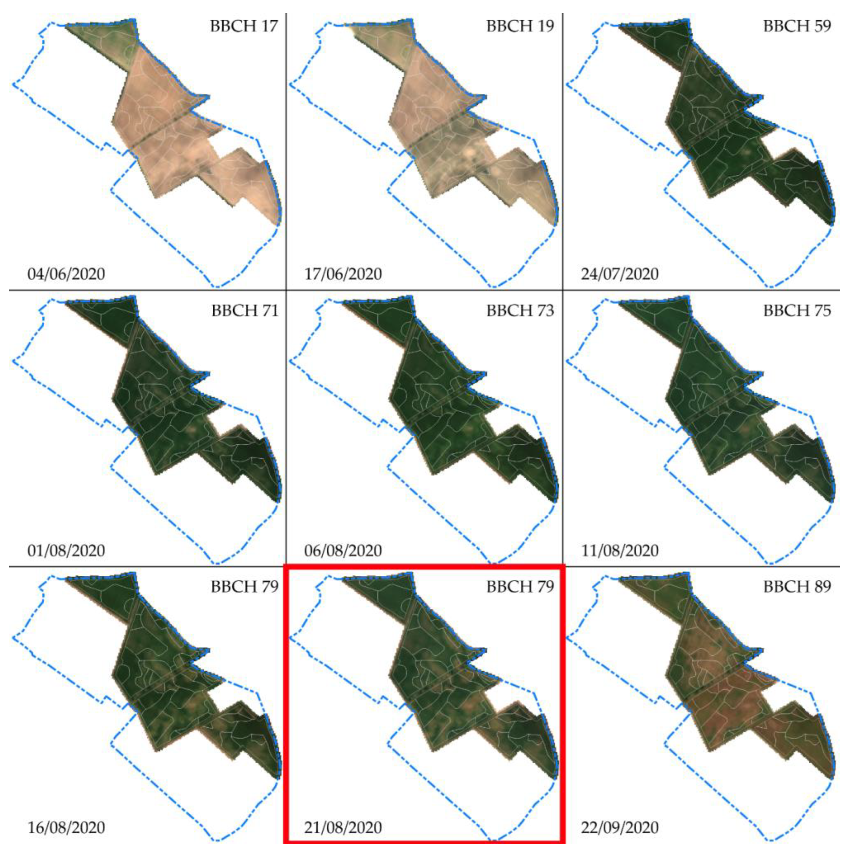
Step 1—Selection of the Sentinel-2 Image on Which the Impact of the Drought Is the Most Visible

According to the hypothesis, the possibility of improving the mapping of soil variability through the analysis of ground surface or canopy images is influenced by two factors: the plant’s developmental stage and the health condition of vegetation determined by soil water deficiency. Consequently, the selection of the best date for further analysis was carried out by interpreting the collected ground data and based on a literature review of water requirements at phenological development stages (BBCH). For a better interpretation of the data obtained from the weather station, a daily climatic water balance (CWB) was calculated to help choose the date of the most intensified drought. The critical water shortage was also defined based on the rules of the Agricultural Drought Monitoring System [19], where the relation between CWB and growth stage allow yield loss caused by drought to be determined. The illustration of the function of this relation is attached in Figure A2 (Appendix C).

The result of this step is the selection of the date with the maximum drought impact observed and consequently selecting the Sentinel-2 image that best fit this period.

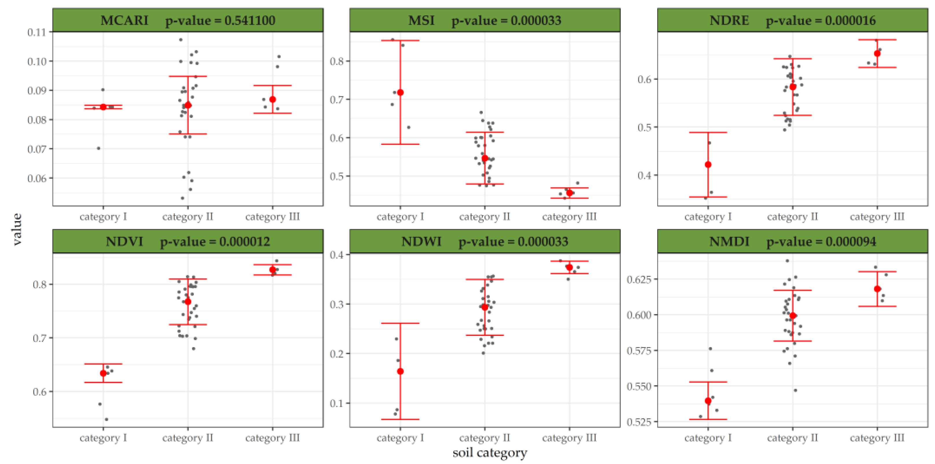
Step 2—Selection the Vegetation Index for the Best Reclassification of the Soil Drought Vulnerability Category Map (Soil-Agricultural Map)

The image from step 1 was processed to six vegetation indicator (VI) raster maps by using Formulas (1)–(6). Statistical distributions of the VI values were estimated for each of the maps, separately for each category (I–III) of drought vulnerability. Because in most cases the variable does not have a normal distribution, median was adopted as a measure of the average value of the distribution and median absolute deviation (MAD) was chosen as the indicator of statistical dispersion and calculated using Formula 7 [60]. A median of the individual VI values was calculated for each contour of the analyzed soil-agricultural map at a scale of 1:25,000 with an assigned soil drought susceptibility category; these values were grouped into the studied soil drought susceptibility categories to which MAD was calculated.

$$\mathrm{M}\mathrm{A}\mathrm{D}=\mathrm{b}{\mathrm{M}}_{\mathrm{i}}\left(\left|{\mathrm{x}}_{\mathrm{i}}-{\mathrm{M}}_{\mathrm{j}}\left({\mathrm{x}}_{\mathrm{j}}\right)\right|\right)$$

(7)

where x_i—n original observations; M_i—median of the series; b—constant.

It was assumed that the best VI map (among six chosen indicators) which can be used for improving the soil drought vulnerability category map would be the one that achieved the best separation of VI values for categories of soil vulnerability to drought. For the analysis of these relationships, visualization of data distributions by box plots was adopted.

The results of this step are as follows:

• The vegetation index map which was chosen as the base to be used for further geoprocessing;
• The reclassification table consisting of three ranges of index values (presented on the box plot) which describe the highest probability of belonging to one of the three soil categories. These ranges of VI index values were obtained by the following Formula (8):

$${\mathrm{c}\mathrm{a}\mathrm{t}\mathrm{g}\mathrm{o}\mathrm{r}\mathrm{y}}_{\mathrm{n}}=\left[\mathrm{M}\left({\mathrm{V}\mathrm{I}}_{{\mathrm{c}\mathrm{a}\mathrm{t}}_{\mathrm{n}}}\right)-\mathrm{M}\mathrm{A}\mathrm{D}\left({\mathrm{V}\mathrm{I}}_{{\mathrm{c}\mathrm{a}\mathrm{t}}_{\mathrm{n}}}\right);\mathrm{M}\left({\mathrm{V}\mathrm{I}}_{{\mathrm{c}\mathrm{a}\mathrm{t}}_{\mathrm{n}}}\right)+\mathrm{M}\mathrm{A}\mathrm{D}\left({\mathrm{V}\mathrm{I}}_{{\mathrm{c}\mathrm{a}\mathrm{t}}_{\mathrm{n}}}\right)\right]$$

(8)

where ${\mathrm{c}\mathrm{a}\mathrm{t}\mathrm{g}\mathrm{o}\mathrm{r}\mathrm{y}}_{\mathrm{n}}$—n soils category; $\mathrm{M}\left({\mathrm{V}\mathrm{I}}_{{\mathrm{c}\mathrm{a}\mathrm{t}}_{\mathrm{n}}}\right)$—median of the series VI for n soils category; $\mathrm{M}\mathrm{A}\mathrm{D}\left({\mathrm{V}\mathrm{I}}_{{\mathrm{c}\mathrm{a}\mathrm{t}}_{\mathrm{n}}}\right)$—mad of the series VI for n soils category.

Step 3—Soil Drought Vulnerability Category Map (Soil-Agricultural Map) Reclassification by Using Selected VI Map

The VI map chosen in step 2 was used for detailing the map of soil vulnerability to drought (input scale at 1:25,000). For this purpose, the reclassification table was used for recalculation. Each pixel of the drought vulnerability category map has been compared with the corresponding pixel of map VI. If the value of the vegetation index corresponded to the range of another soil category (according to the table), the attribute of this pixel on the soil map changed its value according to the relation described in the table. This process can be described by the following reclassification table (

Table 3. Reclassification table.

Old Values	New Values (Soils Category)
$({minVI}_{{cat}_1}-{maxVI}_{{cat}_1})$	1
$({minVI}_{{cat}_2}-{maxVI}_{{cat}_2})$	2
$({minVI}_{{cat}_3}-{maxVI}_{{cat}_3})$	3

).

Finally, each pixel was assigned to the corresponding category (in the table of reclassification). If the value of a pixel was not within the calculated ranges, then the assignments to the category were not changed (the old one was used). The result of this step is a new detailed soil map (map of soil vulnerability to drought).

Step 4—Validation of the Obtained Reclassification

The obtained map (in step 3) was validated through the in-field tests. A random distribution of 30 soil sampling sites was mapped: 15 where reclassification changed the category of soil vulnerability to drought and 15 where there was no change. From each designated site, soil samples were taken in three depths which corresponded to the soil-agricultural map units. A total of 90 soil samples were taken, which were then analyzed in the laboratory. For each sample, the granulometric composition was determined according to the standard used for preparing the soil-agricultural map. Based on the results obtained from the laboratory, the available water capacity was determined for each soil sample according to Formula (9) and the retention parameters of soils [42,61]. Table of parameters is presented in Appendix A (Table A2).

$$\mathrm{A}\mathrm{W}\mathrm{C}=\sum _{\mathrm{i}=1}^{\mathrm{n}}\mathrm{a}\times \mathrm{d}$$

(9)

where n—separate layers of the soil profile; a—parameter corresponding to the soil texture determined in the laboratory (Appendix A Table A2); d—thickness of soil horizon in meters.

Based on these calculations, the analyzed soil profile was attributed to the corresponding drought vulnerability category (Table 1). The result of this step is a statistical assessment of this reclassification process and provides important suggestions for further research.

3. Results

3.1. Step 1 Results

Maize is a plant that needs quite significant supplies of water to build its biomass and grain. These needs increase exponentially until BBCH 55 (middle of tassel emergence: middle of tassel begins to separate); after that, they stabilize at high levels until BBCH 75 (kernels in middle of cob yellowish white), then decrease. However, from BBCH 0 to BBCH 5, total precipitation amounted to almost 109 mm (1.2 mm/day), but during the critical moment of kernel development, from BBCH 5 to BBCH 79, total precipitation equaled about 25 mm (0.7 mm/day). The deficiency of precipitation during this period caused a significant reduction in maize grain yield (

Table 4. Observed phenological development stages of maize in BBCH scale and meteorological conditions.

	Start Day	Duration (No. of Days)	Sum of Precipitation (mm)	avg. max. Temperature (°C)	avg. min. Temperature (°C)	avg. Temperature (°C)	Sum of CWB (-)	CBW per Day (-)	Sum of Precipitation (mm)	Precipitation per Day (mm)
BBCH 00	21 April 2020
		31	24.1	17.4	4.2	11.2	−87.7	−2.8	108.9	1.2
BBCH 1	21 May 2020
		38	44.2	22.0	10.5	16.3	−108.6	−2.9
BBCH 3	27 June 2020
		19	40.6	24.1	12.5	18.2	−41.0	−2.2
BBCH 5	16 July 2020
		10	12.1	25.9	12.3	19.1	−33.3	−3.3	24.7	0.7
BBCH 6	26 July 2020
		9	7.5	25.4	12.1	19.3	−31.5	−3.5
BBCH 7	4 August 2020
		17	5.1	29.6	13.8	22.1	−78.9	−4.4
BBCH 8	22 August 2020
		52	81.1	20.5	10.1	15.2	−47.0	−0.9
BBCH 9	12 October 2020
		7	26.1	10.6	5.6	8.0	19.8	2.8
BBCH 99	19 October 2020

).

Analysis of the rainfall data allowed for the identification of a critical phase in corn development (BBCH 7), and the calculated CWB at the 60-day and 15-day (

Table 5. Date list of analyzed images with CWB in 60-day and 15-day steps.

Sentinel-2 Date	CWB 60 Days	CWB 15 Days	BBCH
4 June 2020	−178.6	−42.5	BBCH 17
17 June 2020	−179.6	−57.0	BBCH 19
24 July 2020	−181.5	−45.5	BBCH 55
1 August 2020	−185.8	−61.0	BBCH 65
6 August 2020	−183.4	−58.0	BBCH 71
11 August 2020	−193.8	−62.7	BBCH 73
16 August 2020	−191.7	−62.9	BBCH 75
21 August 2020	−206.3	−72.2	BBCH 79
22 September 2020	−163.2	−44.6	BBCH 89

) steps allowed a determination of in which image the drought impact was most significant, noting that plants react to a scarcity of water in the soil with some delay.

As in the result of step 1, for further analyses the Sentinel-2 image dated 21 August 2020 was selected.

3.2. Step 2 Results

A soil-agricultural map at a scale of 1:25,000 was overlaid on the selected corn fields, and each of the located polygons was assigned to the corresponding soil drought vulnerability category. Crossing (transition) between the polygons is not direct, so to avoid the impact of the demarcated boundaries, a 10 m buffer was made (Figure 2B).

The medians and MAD were calculated for each soil polygon with an assigned soil category and for each vegetation index. The results were presented in the form of a box-plot chart (Figure 4). These calculated statistics allowed us to choose the vegetation index which gives the best distinction between soil categories and the obtained values were used to reclassify drought vulnerability soil maps. The black dots represent the medians for each polygon, the red dots represent the median for the set of each soil category and the red bars (top and bottom) show the median +/− MAD. The best soil category differentiation was obtained for NDVI, for this index had the lowest p-value (12 × 10⁻⁶) with the Kruskal–Wallis test (Figure 4). The worst class separation was gained for MCARI (p-value = 0.5411).

3.3. Step 3 Results

Reclassification was performed by applying the obtained NDVI values which allowed for the best differentiation of soil categories, the result of which is shown in Figure 5. In the case study, 31% of the areas of the surveyed fields changed their soil drought vulnerability category and 69% kept the category unchanged. Soil drought vulnerability category II was reclassified the most, i.e., 22 ha was transferred to another category (14% to category I and 7% to category III). The reclassification areas for the other categories were 6 ha for category III and 4 ha for category I. Comparing the maps in Figure 5A and 5B, it can be noticed that the soil image has noticeably changed as well, where large homogeneous polygons became mosaicked. Additionally, small clusters of pixels and single pixels have appeared.

3.4. Step 4 Results

Validation based on soil sampling gave quite favorable results. The soil samples were divided into two equal groups (15 each): the first group represented sites where the reclassification changed the soil categories—category modified in Figure 5B (red dots); the second group represented sites where the reclassification did not change the soil category—category unmodified in Figure 5B (blue dots). The validation result was visualized with a box plot, indicating the assignment of each sample to a given category depending on soil properties (AWC). All soil samples for the second group were assigned to the correct soil category (Figure 6B), and for the first group only two samples (marked by red oval in Figure 6A) were between category 1 and category 2 with the borderline values between the ranges.

Additionally, for soil sampling points, between estimated available water content and calculated NDVI values based on Sentinel-2 images, a linear regression curve was determined which showed a significant relationship between the variables (R² = 0.94) (Figure 7).

4. Discussion

4.1. Significance of the Conducted Research and the Possibility of Its Practical Application

Demonstrating the truth of the research hypothesis will enable to initiate extensive work on the development of a new soil map detailing the existing categorization of soil vulnerability to drought based on the proposed methodology for using multispectral Senitel-2 images for the needs of the national drought monitoring system [41].

It is extremely important as this system is currently used to assess crop losses across agricultural parcels. This assessment is the basis for the mechanisms of direct support paid by state authorities to farmers suffering drought losses.

In addition, the introduction of observations of the direct impact of drought on crops into the monitoring system provides the opportunity for dialogue with farmers in the event of discrepancies in assessments between government agencies or companies insuring crops and agricultural producers. This type of situation was described in the paper by Jedrejek et al., 2022 [19], where the authors indicate the possibility of using remote sensing in assessing the regional effects of drought. Extending this method through a comprehensive assessment (water shortage rate and recognition of soil variability) will allow the farmer to directly present evidence for an objective assessment of the impact of drought on his crops and to indicate possible agrotechnology negligence or failure to adapt agrotechnology to the agricultural drought risk prevailing in this region.

Another example of applying the described results in agricultural practice is precision farming. The implementation of precision methods in agriculture requires, on the one hand, correct recognition of the variability of soil conditions and the occurrence of threats (e.g., outbreaks of diseases, occurrence of pests, ranges of hunting losses) and, on the other hand, monitoring the effects of diversifying the application of means of production (fertilizers) and protection (pesticides, herbicides). In the former case, the described methods are directly applicable. In the latter, detailed soil maps can be a reference source for assessing the correctness of the treatments performed and the selection of dose differentiation [62,63].

4.2. The Direction of Future Research

The next phase of research will exactly match the development strategy of the national agricultural drought monitoring system [41]. The methodology presented in this work will be applied to soil remote sensing for the most important types of crops in Poland: cereals (wheat, barley and rye) and rapeseed. Research will also be continued for different maize varieties. The area of research will be extended, because the IV soil drought vulnerability category (which did not occur in the fields of the presented case study) and the specificity of soil diversity in other regions of the country must also be taken into account. Finally, it is assumed that the currently used soil-agriculture maps in the drought monitoring system will be detailed at least ten times, i.e., from the scale of 1:25,000 to the scale of 1:2500. The drought vulnerability map obtained in this way will be made publicly available to farmers, agricultural advisors and insurance companies as part of the Geomatics Center being built at the Institute (IUNG-PIB). This access is planned as an e-service belonging to a wider package of services to be developed and financed under the National Recovery and Resilience Plan funded by the European Union [64].

5. Conclusions

The conducted research fully confirmed the assumptions of the working hypothesis. The analysis of the satellite image, at the selected date, on which the greatest water deficiency in the soil was recorded and, consequently, the stress in the monitored crop was the highest, allowed for a significant improvement in the accuracy of the soil drought vulnerability category map. The direct results of the research are as follows:

• Statement of the possibility of recognizing the soil mosaic with spatial accuracy of the Sentinel-2 image;
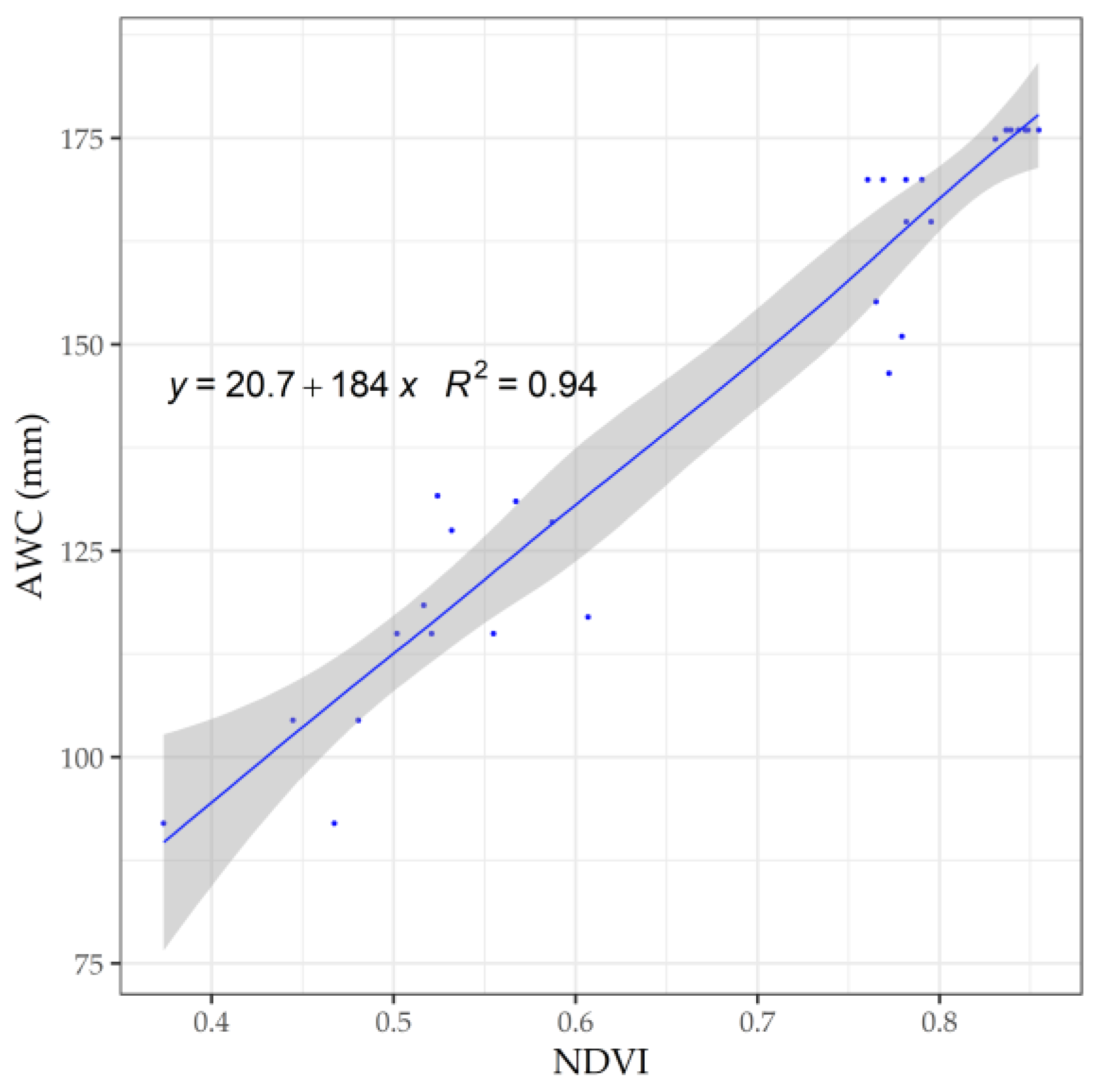
• Indication of the NDVI index as the best indicator of the diversity of greenness caused by water stress.

Research will be continued in order to build a general model for reclassification of the soil and agricultural map based on full satellite monitoring of the country.

References

1. FAO-UNESCO. Soil Map of the World, 1:5,000,000 Volume I Legend; FAO-UNESCO: Rome, Italy, 1974; ISBN 92-3-101125-1. [Google Scholar]
2. Batjes, N.H. A World Dataset of Derived Soil Properties by FAO-UNESCO Soil Unit for Global Modelling. Soil Use Manag. 1997, 13, 9–16. [Google Scholar] [CrossRef]
3. FAO-UNESCO. Revised Legend of the FAO-UNESCO Soil Map of the World; World soil resources report 60; FAO-UNESCO: Rome, Italy, 1988; p. 110. [Google Scholar]
4. Stolt, M.H.; Needelman, B.A. Fundamental Changes in Soil Taxonomy. Soil Sci. Soc. Am. J. 2015, 79, 1001–1007. [Google Scholar] [CrossRef]
5. Soil Survey Staff Soil Taxonomy. A Basic of Soil Classification for Making and Interpreting Soil Surveys; Soil Conservation Service, U.S. Dept. of Agriculture: Singapore, 1975. [Google Scholar]
6. Soil Survey Staff. Keys to Soil Taxonomy; USDA-Natural Resources Conservation Service: Washington, DC, USA, 2014.
7. Salehi, M.H. Challenges of Soil Taxonomy and WRB in Classifying Soils: Some Examples from Iranian Soils. Bull. Geogr. Phys. Geogr. Ser. 2018, 14, 63–70. [Google Scholar] [CrossRef] [Green Version]
8. Schad, P. World Reference Base for Soil Resources. In Reference Module in Earth Systems and Environmental Sciences; Elsevier: Amsterdam, The Netherlands, 2017; ISBN 978-0-12-409548-9. [Google Scholar]
9. IUSS Working Group. WRB World Reference Base for Soil Resources 2014, Update 2015 International Soil Classification System for Naming Soils and Creating Legends for Soil Maps; World Soil Resources Reports No. 106; FAO: Rome, Italy, 2015. [Google Scholar]
10. Strzemski, M. Pulawski Period of Dokuchaev’s Activities [in Polish—Puławski Okres Działalności Dokuczajewa]. Postępy Wiedzy Rol. 1952, 04, 4. [Google Scholar]
11. Regulation of the Council of Ministers of 4 June 1956 Regarding Land Classification [In Polish—Rozporządzenie Rady Ministrów z Dnia 4 Czerwca 1956 r. w Sprawie Klasyfikacji Gruntów]. Dz.U. z. 1959 Nr. 19 Poz. 97. 1956. Available online: https://isap.sejm.gov.pl/isap.nsf/DocDetails.xsp?id=wdu19560190097 (accessed on 12 January 2023).
12. Smreczak, B.; Łachacz, A. Soil types specified in the bonitation classification and their analogues in the sixth edition of the Polish Soil Classification [in Polish—Typy gleb wyróżniane w klasyfikacji bonitacyjnej i ich odpowiedniki w 6. wydaniu Systematyki gleb Polski]. Soil Sci. Annu. 2019, 70, 115–136. [Google Scholar] [CrossRef]
13. Strzemski, M.; Bartoszewski, Z.; Czarnowski, F.; Dombek, E.; Siuta, J.; Truszkowska, R.; Witek, T. Instruction Regarding the Preparation of Soil-Agricultural Maps on a Scale of 1:5000 and 1:25,000 and Soil-Agricultural Maps on a Scale of 1:25,000. Appendix to Regulation No. 115 of the Minister of Agriculture of 28 July 1964 Concerning the Organisation of Soil-Agricultural and Agricultural-Cartographic Works [In Polish—Instrukcja w Sprawie Wykonywania Map Glebowo-Rolniczych w Skali 1:5000 i 1:25,000 Oraz Map Glebowo-Przyrodniczych w Skali:1:25,000. Załącznik Do Zarządzenia Nr 115 Ministra Rolnictwa z Dnia 28 Lipca 1964 r. w Sprawie Organizacji Prac Gleboznawczo- i Rolniczo-Kartograficznych]. Dz.Urz. Min. Rol. Nr. 19 Poz. 121 1964. [Google Scholar]
14. Strzemski, M.; Siuta, J.; Witek, T. Agricultural Suitability of Polish Soils [In Polish—Przydatność Rolnicza Gleb Polski]; PWRiL: Warszawa, Poland, 1973. [Google Scholar]
15. Witek, T.; Górski, T. Evaluation of the Natural Capability of Agricultural Areas in Poland; Wydawnictwa Geologiczne: Warszawa, Poland, 1977. [Google Scholar]
16. Witek, T. The content and methodologies used for large-scale soil and agricultural mapping [in Polish—Treść i metody sporządzania wielkoskalowych map glebowo-rolniczych]. Rocz. Glebozn. 1965, 40, 99–117. [Google Scholar]
17. ADMS—Soil Categories. Available online: https://susza.iung.pulawy.pl/en/kategorie/ (accessed on 20 December 2022).
18. Doroszewski, A.; Jadczyszyn, J.; Kozyra, J.; Pudełko, R.; Stuczyński, T.; Mizak, K.; Łopatka, A.; Koza, P.; Górski, T.; Wróblewska, E. Fundamentals of a Agricultural Drought Monitoring System [in Polish—Podstawy Systemu Monitoringu Suszy Rolniczej]. Woda-Śr.-Obsz. Wiej. 2012, 12, 77–91. [Google Scholar]
19. Jędrejek, A.; Koza, P.; Doroszewski, A.; Pudełko, R. Agricultural Drought Monitoring System in Poland—Farmers’ Assessments vs. Monitoring Results (2021). Agriculture 2022, 12, 536. [Google Scholar] [CrossRef]
20. Bartosiewicz, B.; Jadczyszyn, J. The Impact of Drought Stress on the Production of Spring Barley in Poland. Pol. J. Agron. 2021, 45, 3–11. [Google Scholar] [CrossRef]
21. Zhou, Y.; Wu, W.; Liu, H. Exploring the Influencing Factors in Identifying Soil Texture Classes Using Multitemporal Landsat-8 and Sentinel-2 Data. Remote Sens. 2022, 14, 5571. [Google Scholar] [CrossRef]
22. Belmonte, A.; Riefolo, C.; Lovergine, F.; Castrignanò, A. Geostatistical Modelling of Soil Spatial Variability by Fusing Drone-Based Multispectral Data, Ground-Based Hyperspectral and Sample Data with Change of Support. Remote Sens. 2022, 14, 5442. [Google Scholar] [CrossRef]
23. Abdellatif, M.A.; El Baroudy, A.A.; Arshad, M.; Mahmoud, E.K.; Saleh, A.M.; Moghanm, F.S.; Shaltout, K.H.; Eid, E.M.; Shokr, M.S. A GIS-Based Approach for the Quantitative Assessment of Soil Quality and Sustainable Agriculture. Sustainability 2021, 13, 13438. [Google Scholar] [CrossRef]
24. Crema, A.; Boschetti, M.; Nutini, F.; Cillis, D.; Casa, R. Influence of Soil Properties on Maize and Wheat Nitrogen Status Assessment from Sentinel-2 Data. Remote Sens. 2020, 12, 2175. [Google Scholar] [CrossRef]
25. Sorenson, P.T.; Kiss, J.; Bedard-Haughn, A.K.; Shirtliffe, S. Multi-Horizon Predictive Soil Mapping of Historical Soil Properties Using Remote Sensing Imagery. Remote Sens. 2022, 14, 5803. [Google Scholar] [CrossRef]
26. Gasmi, A.; Gomez, C.; Chehbouni, A.; Dhiba, D.; Elfil, H. Satellite Multi-Sensor Data Fusion for Soil Clay Mapping Based on the Spectral Index and Spectral Bands Approaches. Remote Sens. 2022, 14, 1103. [Google Scholar] [CrossRef]
27. Santaga, F.S.; Agnelli, A.; Leccese, A.; Vizzari, M. Using Sentinel-2 for Simplifying Soil Sampling and Mapping: Two Case Studies in Umbria, Italy. Remote Sens. 2021, 13, 3379. [Google Scholar] [CrossRef]
28. Grzyb, A.; Wolna-Maruwka, A.; Łukowiak, R.; Ceglarek, J. Spatial and Temporal Variability of the Microbiological and Chemical Properties of Soils under Wheat and Oilseed Rape Cultivation. Agronomy 2022, 12, 2259. [Google Scholar] [CrossRef]
29. Lacerda, M.P.C.; Demattê, J.A.M.; Sato, M.V.; Fongaro, C.T.; Gallo, B.C.; Souza, A.B. Tropical Texture Determination by Proximal Sensing Using a Regional Spectral Library and Its Relationship with Soil Classification. Remote Sens. 2016, 8, 701. [Google Scholar] [CrossRef] [Green Version]
30. Gallo, B.C.; Demattê, J.A.M.; Rizzo, R.; Safanelli, J.L.; Mendes, W.D.S.; Lepsch, I.F.; Sato, M.V.; Romero, D.J.; Lacerda, M.P.C. Multi-Temporal Satellite Images on Topsoil Attribute Quantification and the Relationship with Soil Classes and Geology. Remote Sens. 2018, 10, 1571. [Google Scholar] [CrossRef]
31. Bautista, A.S.; Fita, D.; Franch, B.; Castiñeira-Ibáñez, S.; Arizo, P.; Sánchez-Torres, M.J.; Becker-Reshef, I.; Uris, A.; Rubio, C. Crop Monitoring Strategy Based on Remote Sensing Data (Sentinel-2 and Planet), Study Case in a Rice Field after Applying Glycinebetaine. Agronomy 2022, 12, 708. [Google Scholar] [CrossRef]
32. Ayalew, D.A.; Deumlich, D.; Šarapatka, B.; Doktor, D. Quantifying the Sensitivity of NDVI-Based C Factor Estimation and Potential Soil Erosion Prediction Using Spaceborne Earth Observation Data. Remote Sens. 2020, 12, 1136. [Google Scholar] [CrossRef] [Green Version]
33. Attarzadeh, R.; Amini, J.; Notarnicola, C.; Greifeneder, F. Synergetic Use of Sentinel-1 and Sentinel-2 Data for Soil Moisture Mapping at Plot Scale. Remote Sens. 2018, 10, 1285. [Google Scholar] [CrossRef] [Green Version]
34. Copernicu Open Access Hub. Available online: https://scihub.copernicus.eu/dhus/#/home (accessed on 20 December 2022).
35. Hejmanowska, B.; Kramarczyk, P.; Głowienka, E.; Mikrut, S. Reliable Crops Classification Using Limited Number of Sentinel-2 and Sentinel-1 Images. Remote Sens. 2021, 13, 3176. [Google Scholar] [CrossRef]
36. Panek, E.; Gozdowski, D.; Stępień, M.; Samborski, S.; Ruciński, D.; Buszke, B. Within-Field Relationships between Satellite-Derived Vegetation Indices, Grain Yield and Spike Number of Winter Wheat and Triticale. Agronomy 2020, 10, 1842. [Google Scholar] [CrossRef]
37. Solon, J.; Borzyszkowski, J.; Bidłasik, M.; Richling, A.; Badora, K.; Balon, J.; Brzezińska-Wójcik, T.; Chabudziński, Ł.; Dobrowolski, R.; Grzegorczyk, I.; et al. Physico-Geographical Mesoregions of Poland: Verification and Adjustment of Boundaries on the Basis of Contemporary Spatial Data. Geogr. Pol. 2018, 91, 143–170. [Google Scholar] [CrossRef]
38. Marks, L. Pleistocene Glacial Limits in the Territory of Poland. Przegląd Geol. 2005, 53, 988–993. [Google Scholar]
39. Dzięciołowski, W. The soil forming environment and soils of the Wielkopolska Lowlands [in Polish—Środowisko glebotwórcze i gleby Niziny Wielkopolskiej]. Rocz. Glebozn. 1979, XXX, 11–33. [Google Scholar]
40. Local Data Repository, Statistics Poland. Available online: https://bdl.stat.gov.pl/bdl (accessed on 20 December 2022).
41. ADMS—Agricultural Drought Monitoring System. Available online: https://susza.iung.pulawy.pl/en/ (accessed on 20 December 2022).
42. Ślusarczyk, E. Identification of the Useful Retention of Mineral Soils for Forecasting and Irrigation Planning [in Polish—Określenie Retencji Użytecznej Gleb Mineralnych Dla Prognozowania i Projektowania Nawodnień]. Melior. Rolne 1979, 3, 1–10. [Google Scholar]
43. Szewczak, K.; Łoś, H.; Pudełko, R.; Doroszewski, A.; Gluba, Ł.; Łukowski, M.; Rafalska-Przysucha, A.; Słomiński, J.; Usowicz, B. Agricultural Drought Monitoring by MODIS Potential Evapotranspiration Remote Sensing Data Application. Remote Sens. 2020, 12, 3411. [Google Scholar] [CrossRef]
44. Zotarelli, L.; Dukes, M.D.; Romero, C.C.; Migliaccio, K.W.; Kelly, T.M. Step by Step Calculation of the Penman-Monteith Evapotranspiration (FAO-56 Method). Inst. Food Agric. Sci. Univ. Fla. 2015, AE459, 1–10. Available online: https://www.agraria.unirc.it/documentazione/materiale_didattico/1462_2016_412_24509.pdf (accessed on 12 January 2023).
45. Doroszewski, A.; Górski, T. A Simple Index of Potential Evapotranspiration [in Polish—Prosty Wskaźnik Ewapotranspiracji Potencjalnej]. Rocz. Akad. Rol. W Poznaniu. Melior. I Inżynieria Sr. 1995, 16, 3–8. [Google Scholar]
46. Meier, U. Growth Stages of Mono- and Dicotyledonous Plants: BBCH Monograph; Open Agrar Repositorium: Quedlinburg, Germany, 2018. [Google Scholar] [CrossRef]
47. User Guides—Sentinel-2 MSI—Sentinel Online—Sentinel Online. Available online: https://sentinels.copernicus.eu/web/sentinel/user-guides/sentinel-2-msi (accessed on 20 December 2022).
48. Ranghetti, L.; Boschetti, M.; Nutini, F.; Busetto, L. “Sen2r”: An R Toolbox for Automatically Downloading and Preprocessing Sentinel-2 Satellite Data. Comput. Geosci. 2020, 139, 104473. [Google Scholar] [CrossRef]
49. IDB—Index DataBase. Available online: https://www.indexdatabase.de/ (accessed on 22 December 2020).
50. Lin, Y.; Zhu, Z.; Guo, W.; Sun, Y.; Yang, X.; Kovalskyy, V. Continuous Monitoring of Cotton Stem Water Potential Using Sentinel-2 Imagery. Remote Sens. 2020, 12, 1176. [Google Scholar] [CrossRef] [Green Version]
51. Waqas, M.A.; Wang, X.; Zafar, S.A.; Noor, M.A.; Hussain, H.A.; Azher Nawaz, M.; Farooq, M. Thermal Stresses in Maize: Effects and Management Strategies. Plants 2021, 10, 293. [Google Scholar] [CrossRef]
52. Mezera, J.; Lukas, V.; Horniaček, I.; Smutný, V.; Elbl, J. Comparison of Proximal and Remote Sensing for the Diagnosis of Crop Status in Site-Specific Crop Management. Sensors 2021, 22, 19. [Google Scholar] [CrossRef] [PubMed]
53. Tucker, C.J. Red and Photographic Infrared Linear Combinations for Monitoring Vegetation. Remote Sens. Environ. 1979, 8, 127–150. [Google Scholar] [CrossRef] [Green Version]
54. Barnes, E.; Clarke, T.; Richards, S.; Colaizzi, P.; Haberland, J.; Kostrzewski, M.; Waller, P.; Choi, C.; Riley, E.; Thompson, T.; et al. Coincident Detection Of Crop Water Stress, Nitrogen Status And Canopy Density Using Ground-Based Multispectral Data. In Proceedings of the Fifth International Conference on Precision Agriculture, Bloomington, MN, USA, 16–19 July 2000. [Google Scholar]
55. Daughtry, C.S.T.; Walthall, C.L.; Kim, M.S.; de Colstoun, E.B.; McMurtrey, J.E. Estimating Corn Leaf Chlorophyll Concentration from Leaf and Canopy Reflectance. Remote Sens. Environ. 2000, 74, 229–239. [Google Scholar] [CrossRef]
56. Żelazny, W.R.; Lukáš, J. Drought Stress Detection in Juvenile Oilseed Rape Using Hyperspectral Imaging with a Focus on Spectra Variability. Remote Sens. 2020, 12, 3462. [Google Scholar] [CrossRef]
57. Hunt, E.R.; Rock, B.N. Detection of Changes in Leaf Water Content Using Near- and Middle-Infrared Reflectances. Remote Sens. Environ. 1989, 30, 43–54. [Google Scholar] [CrossRef]
58. Gao, B.C. NDWI—A Normalized Difference Water Index for Remote Sensing of Vegetation Liquid Water from Space. Remote Sens. Environ. 1996, 58, 257–266. [Google Scholar] [CrossRef]
59. Wang, L.; Qu, J.J. NMDI: A Normalized Multi-Band Drought Index for Monitoring Soil and Vegetation Moisture with Satellite Remote Sensing. Geophys. Res. Lett. 2007, 34, L20405. [Google Scholar] [CrossRef]
60. Leys, C.; Ley, C.; Klein, O.; Bernard, P.; Licata, L. Detecting Outliers: Do Not Use Standard Deviation around the Mean, Use Absolute Deviation around the Median. J. Exp. Soc. Psychol. 2013, 49, 764–766. [Google Scholar] [CrossRef] [Green Version]
61. Łopatka, A.; Stuczyński, T.; Czyż, E.; Kozyra, J.; Jadczyszyn, J. Analysis the Water Conditions of Soils and Drought-Related Hazards on the Example of Podlaskie Voivodeship (in Polish Analiza Warunków Wodnych Gleb i Zagrożeń Związanych z Suszą Na Przykładzie Województwa Podlaskiego). Stud. Rap. IUNG-PIB 2007, 5, 79–105. [Google Scholar]
62. Pudełko, R.; Niedźwiecki, J.; Debaene, G.; Igras, J.; Kubsik, K. The Remote Sensing Assessment of Potential Productivity of a Field with Soil Spatial Variability. J. Food Agric. Environ. 2012, 10, 790–793. [Google Scholar]
63. Pudełko, R.; Stuczynski, T.; Borzecka, M. The Suitability of an Unmanned Aerial Vehicle (UAV) for the Evaluation of Experimental Fields and Crops. Zemdirbyste 2012, 990014, 431–436. [Google Scholar]
64. Recovery and Resilience Plan for Poland. Available online: https://commission.europa.eu/business-economy-euro/economic-recovery/recovery-and-resilience-facility/recovery-and-resilience-plan-poland_en (accessed on 20 December 2022).
Figure 1. Localization of the study area—Baborówko Experimental Station (BES).
Remotesensing 15 01281 g001
Figure 2. Soil-agricultural map (A) and soil drought vulnerability category map (B) for the study area in Baborówko Experimental Station.
Remotesensing 15 01281 g002
Figure 3. The steps of the analysis.
Remotesensing 15 01281 g003
Figure 4. Comparison of obtained results for selected vegetation indices in each soil category (median +/− MAD) and p-value in the Kruskal–Wallis test.
Remotesensing 15 01281 g004
Figure 5. Drought vulnerability polygons of soils before reclassification (A), after reclassification with soil sampling locations (B).
Remotesensing 15 01281 g005
Figure 6. Validation results of 30 soil samples with: modified category (A) and unmodified category (B).
Remotesensing 15 01281 g006
Figure 7. Diagram of the relationship between NDVI and AWC values.
Remotesensing 15 01281 g007