Rapid Detection and Orbital Parameters’ Determination for Fast-Approaching Non-Cooperative Target to the Space Station Based on Fly-around Nano-Satellite

Abstract

Non-cooperative targets, such as space debris, defunct spacecrafts and LEO constellation satellites, have brought serious risks to the space station. The rapid detection and orbital parameters’ determination of the fast-approaching non-cooperative target can greatly improve the protection ability of the space station. In this paper, a novel rapid detection and orbital parameters’ determination method based on the collaborative observation of the space station, and a fly-around nano-satellite is developed. The early-warning region of the space station is established, and considering the observation constraints of the nano-satellite, the non-cooperative target detection strategy is provided, which includes a collaborative observation configuration as well as the attitude variation of the cameras, and the detection efficiency is analyzed. Then, the orbital parameters’ filtering model of the non-cooperative target based on the collaborative observation is constructed, and the Unscented Kalman filter method is utilized to determinate the orbital parameters of the non-cooperative target. Considered the observability of the initial collaborative observation configuration, this paper analyzes the observation configuration with low observability in different scenarios, and proposes an optimal orbital maneuver algorithm for the nano-satellite. This algorithm can realize a fuel-optimal orbital maneuver that satisfies the minimum line-of-sight angle constraint of the collaborative observation.

1. Introduction

As there is an increasing number of space non-cooperative targets, such as space debris and defunct satellites, the space environment is becoming increasingly crowded [1,2,3]. In May 2021, the Canadarm2 of the International Space Station was hit by space debris and caused visible damage, as shown in Figure 1. In order to avoid the collision threat, it is necessary to detect and identify the approaching non-cooperative target as early as possible, so as to improve the early-warning capability of the space station [4]. With advantages of a small size and low cost, Fly-round nano-satellites can be released in the orbit directly and detect the noncooperative target approaching the space station [5,6].

There are a few measurement methods for the on-orbit space non-cooperative target detection, including a remote ranging measurement using an on-board radar and angle measurement using an on-board camera [7]. Considering the limited carrying capacity of the nano-satellite, it does not have the ability of remote ranging, and the optical angle camera has the advantages of high precision, small size and light weight [8]. Therefore, in order to identify the orbital parameters of the non-cooperative target, the optical angle camera can be equipped with the nano-satellite, and the angle information can be utilized to achieve the accurate positioning of the target.

Woffinden [9,10,11] systematically studied angles-only relative navigation, proposed the solution framework of angles-only relative navigation, deduced the observable criterion of angles-only relative navigation, and studied the optimal orbital maneuver strategy to improve the observability of angles-only navigation. Only two angular measurements can be obtained by using a single camera to observe the non-cooperative target, the observation geometric performance is limited and the filtering process is unstable. Aiming at the problem of a low precision of single satellite angles-only tracking, Gong et al. [12] proposed a novel consensus-constrained relative navigation algorithm based on the lever arm effect of the sensor offset from the spacecraft center of mass. Yao et al. [13] proposed a method of the collaborative tracking of the non-cooperative target by using formation satellites, and the Square-Root Cubature Kalman Filter (SRCKF) method is used to realize the angles-only navigation of a non-cooperative target. Binocular or multi-view collaboration observation can greatly improve the observation geometric performance, and improve the stability of the orbital parameters’ identification. Meanwhile, it increases the complexity of the observation system. Han et al. [14] used the EKF method to study the angles-only navigation of the space non-cooperative target by multi-view collaborative observation. Aiming at the problem that a weak observation exists along the range direction when the line-of-sight angle is used as the measurement information for medium range relative navigation, Wang et al. [15] studied an autonomous double line-of-sight measurement and relative navigation method based on the formation of the dual chase spacecraft. Su et al. [16] studied the ranging relative navigation of the non-cooperative target based on formation satellites, and analyzed the observability through the line-of-sight (LOS) angle of collaborative observation; they concluded that within the range of [0°, 90°], the observability improves with the increase in the collaborative LOS angle, but they did not propose an improvement method for the case of low observability. From the study of second-order nonlinear relative motion dynamics in the Cartesian coordinate system, Kaufman et al. [17] studied the nonlinear observability problem of the angle-only relative orbital determination by using a high-order Lie derivative. Li et al. [18] demonstrated that the nonlinear model can solve the unobservable problem of angle-only relative navigation in the Cartesian coordinate system. At present, many scholars have studied the methods to improve the observability of angles-only relative navigation, such as the orbital maneuver method [19], camera offset method [20], nonlinear dynamics method [21] and multi-sensor method [22].

Aiming at the rapid detection and orbital parameters’ determination of the fast-approaching non-cooperative target, this paper proposes a novel rapid detection and orbital parameters’ determination method based on the collaborative observation of the nano-satellite and space station. The measurement model in this paper is a nonlinear equation. The Kalman filter (KF) is suitable for the linear model, and it needs to be linearized for the nonlinear model, which will affect the accuracy. The unscented Kalman filter (UKF) is suitable for the nonlinear model, which not only avoids the truncation error caused by linearization, but also does not need to calculate the Jacobian matrix of the measurement equation, which reduces the complexity of the calculation. Therefore, this paper uses the UKF algorithm to estimate the orbital parameters. The fly-around configuration of the nano-satellite and the space station is designed for the coverage scanning of the early-warning region around the space station. Then, the orbital parameters’ filtering model of the non-cooperative target is established, and the Unscented Kalman filter (UKF) method is utilized to determinate the orbital parameters. The accuracy of the filter is analyzed, and the minimum angle between the fly-around nano-satellite observation direction and the space station observation direction is developed. In addition, considered the low observability, the scheme to improve the observability is developed, and an optimal orbital maneuver by the nano-satellite is proposed.

This paper is organized as follows. Section 2 introduces the problem description and the establishment of relevant models, including the dynamic model of the relative motion, the filtering model of orbital parameters and the optimal model of the orbital maneuver. Section 3 introduces the collaborative detection scheme of the early-warning region. Section 4 introduces the UKF method for orbital parameters’ determination. Simulation results are conducted to validate the proposed method in Section 5. Section 6 concludes this paper.

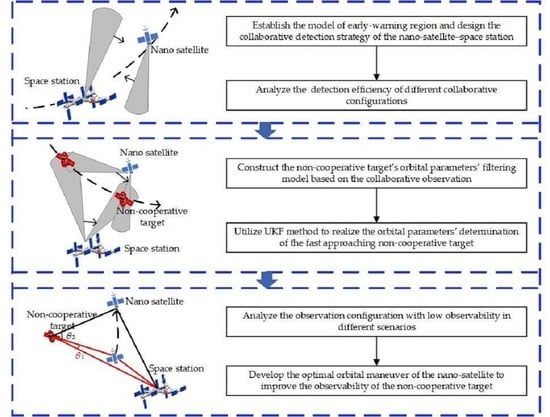
2. Problem Description and Model Establishment

The problem of the non-cooperative target detection and orbital parameters’ determination for the rapid proximity to the space station can be divided into three parts: ① As shown in Figure 2a, use cameras on the space station and nano-satellite to scan the early-warning region around the space station, and detect the approaching non-cooperative target in time; ② as shown in Figure 2b, realize the orbital parameters’ determination of the non-cooperative target based on the collaborative observation of the nano-satellite–space station; ③ as shown in Figure 2c, for the observation configuration with low observability, design the impulsive maneuver of the nano-satellite to ameliorate the collaborative observation configuration, so as to improve the observability.

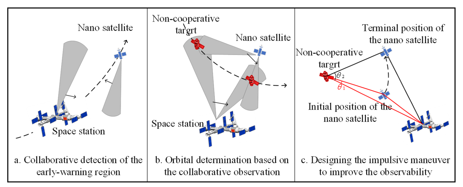
2.1. Collaboration Detection of the Early-Warning Region

In order to scan and detect the early-warning region around the space station, the collaborative detection scheme should be determined by combining the adjoint orbit of the nano-satellite relative to the space station and the camera scanning rule of the nano-satellite–space station.

Considering that the space station is in a near-circular orbit, the law of relative motion between the nano-satellite and the space station approximately satisfies the C-W equation. The local horizontal local vertical coordinate system (LVLH) of the space station is used as the coordinate system to describe the relative motion. Its origin is located at the centric of the space station. The x-axis points radially to the space station from the centric of the Earth. The y-axis is on the orbital plane and points to the velocity direction of the trajectory, and the z-axis is perpendicular to the orbit plane. Without considering the effects of the active control and perturbation, the C-W equation can be described as [23]:

$$\{\begin{array}{l}\ddot{x}-2n\dot{y}-3n^{2}x=0\\ \ddot{y}+2n\dot{x}=0\\ \ddot{z}+n^{2}z=0\end{array}$$

(1)

where n is the orbital angular velocity of the space station, ${[x,y,z]}^T$ represent the relative position of the nano-satellite.

The homogeneous Equation (1) is solved to obtain its analytical solution:

$$\{\begin{array}{l}x=\frac{{\dot{x}}_0}{n}\sin nt-\left(\frac{2}{n}{\dot{y}}_0+3x_0\right)\cos nt+2\left(2x_0+\frac{{\dot{y}}_0}{n}\right)\\ y=2\left(\frac{2}{n}{\dot{y}}_0+3x_0\right)\sin nt+\frac{2}{n}{\dot{x}}_0\cos nt-3\left({\dot{y}}_0+2n{x}_0\right)t+\left(y_0-\frac{2}{n}{\dot{x}}_0\right)\\ z=\frac{{\dot{z}}_0}{n}\sin nt+z_0\cos nt\\ \dot{x}=\left(2{\dot{y}}_0+3n{x}_0\right)\sin nt+{\dot{x}}_0\cos nt\\ \dot{y}=-2{\dot{x}}_0\sin nt+\left(4{\dot{y}}_0+6n{x}_0\right)\cos nt-3\left({\dot{y}}_0+2n{x}_0\right)\\ \dot{z}=-n{z}_0\sin nt+{\dot{z}}_0\cos nt\end{array}$$

(2)

It is worth noting that in the analytical solution (2), the y direction (forward direction) contains the long-term term $-3\left({\dot{y}}_0+2n{x}_0\right)t$; the relative motion between the satellite and space station will increase with time in the y direction. In order to maintain the formation configuration and construct the periodic orbit, the influence of the long-term term must be eliminated, that is,

$${\dot{y}}_0=-2n{x}_0$$

(3)

By eliminating the aperiodic term from the analytical solution, the periodic solution can be obtained as Equation (4).

$$\{\begin{array}{l}x=x_0\cos nt+\frac{{\dot{x}}_0}{n}\sin nt\\ y=-2x_0\sin nt+2\frac{{\dot{x}}_0}{n}\cos nt+(y_0-\frac{2{\dot{x}}_0}{n})\\ z=z_0\cos nt+\frac{{\dot{z}}_0}{n}\sin nt\\ \dot{x}=-n{x}_0\sin nt+{\dot{x}}_0\cos nt\\ \dot{y}=-2n{x}_0\cos nt-2{\dot{x}}_0\sin nt\\ \dot{z}=-n{z}_0\sin nt+{\dot{z}}_0\cos nt\end{array}$$

(4)

It can be observed from the above that different configuration schemes can be obtained by designing the relative orbital information between the nano-satellite and the space station.

In addition to the collaborative configuration between the nano-satellite and the space station, the attitude variation of the cameras on the nano-satellite and the space station should also be considered. To ensure the coverage scanning of the early-warning region, the camera needs to scan both inside and outside the orbital plane of the space station. Therefore, the camera attitude changes adopt the following rule:

$$\left[\begin{array}{c}{\gamma }_m(t)\\ {\theta }_m(t)\end{array}\right]=\left[\begin{array}{c}{\gamma }_0\cdot \cos (\omega t)\\ {\theta }_0\sin (\omega t)\end{array}\right]$$

(5)

where ${\gamma }_m$ and ${\theta }_m$ are the vertical angle and azimuth angle of the viewing field direction of the camera, respectively; ${\gamma }_0$ and ${\theta }_0$ are the maximum values of the camera swing range, which are determined by the constraint of the camera swing amplitude; and $\omega$ is the swing angular velocity of the camera.

Combined with the collaborative detection configuration of the nano-satellite–space station and the variation rule of the camera attitude, the collaborative detection scheme for the early-warning region can be determined.

2.2. Orbital Parameters’ Filtering Model of Non-Cooperative Target Based on the Dual-View Angle Information

The angle information of the non-cooperative target is obtained through the collaborative observation of the target, and then the orbital parameters of the non-cooperative target is estimated by the Unscented Kalman filter. The state model and measurement model of the filtering process are given here.

The relative position and velocity between the target and the space station are taken as the state variable to construct the system model, defined as $\mathit{X}=[{\mathit{r}}^{\mathrm{T}},{\mathit{v}}^{\mathrm{T}}]$. The target estimation model can be expressed as

$${\mathit{X}}_{k+1}=f({\mathit{X}}_k)+{\mathit{\omega }}_k$$

(6)

the estimation model; namely, the state transfer equation can be obtained according to the C-W equation, where ${\mathit{X}}_k$ is the system state vector at time k, and ${\mathit{\omega }}_k$ is the system noise.

The geometric relationship of the dual-view observation is shown in Figure 3. The subscript c and co represent the camera coordinate system of the space station and the nano-satellite, respectively. $\theta$ and $\gamma$ represent the azimuth angle and vertical angle of the observation camera relative to the target, respectively. Taking the vertical angle and azimuth angle of the non-cooperative target as the observation variable, it is defined as $\mathit{Z}={[{\gamma }_c,{\theta }_c,{\gamma }_{co},{\theta }_{co}]}^{\mathrm{T}}$.

The measurement model is the mapping relationship between the target state information and the measurement information, as shown in Equation (7), where ${\mathit{v}}_k$ is the measurement noise. ${\mathit{l}}_C={\left[x_c,y_c,z_c\right]}^{\mathrm{T}}$ is the observation vector in the camera coordinate system of the space station, and ${\mathit{l}}_{co}={\left[x_{co},y_{co},z_{co}\right]}^{\mathrm{T}}$ is the observation vector in the camera coordinate system of the nano-satellite.

$${\mathit{Z}}_k=\left[\begin{array}{c}{\gamma }_c\\ {\theta }_c\\ {\gamma }_{co}\\ {\theta }_{co}\end{array}\right]=\left[\begin{array}{l}\begin{array}{c}\arctan \left(x_c/y_c\right)\\ \arctan \left(z_c/\sqrt{x_c^2+y_c^2}\right)\end{array}\\ \begin{array}{c}\arctan \left(x_{co}/y_{co}\right)\\ \arctan \left(z_{co}/\sqrt{x_{{}_{co}}^2+y_{{}_{co}}^2}\right)\end{array}\end{array}\right]+{\mathit{v}}_k$$

(7)

2.3. Orbital Maneuvering Optimization of the Nano-Satellite Considering the Observability of Non-Cooperative Target

Based on the collaborative observation of the dual-view, the line-of-sight (LOS) angle of the collaborative observation will affect its observability. The measurement system has a low observability when the LOS angle of collaborative observation is close to π or 0. Here, the LOS angle of the collaborative observation is defined as: the angle between the observation direction of the space station and the observation direction of the nano-satellite. As shown in Figure 2c, the LOS angle of the collaborative observation is ${\theta }_1$ at the initial time, which is close to 0°, and the system has low observability. Thus, the nano-satellite needs to improve the observability through changing the LOS angle of the collaborative observation. There are numerous possible terminal states for the nano-satellite’s maneuver. How to select the terminal state of the nano-satellite’s maneuver can obtain the optimal observation configuration with the minimum energy consumption, which is the key to solving this problem. In view of the above problems, this paper proposes to improve the observability through the orbital maneuver of the nano-satellite. The fuel consumption and the improvement of observability is taken as the performance index, and the terminal state of the nano-satellite’s maneuver is analyzed to obtain the optimal performance index.

2.3.1. Orbital Maneuver Optimization

• Orbital maneuver scheme:

For the convenience of analysis, two typical collaborative configurations are considered to describe the orbital maneuver scenario: (a) The nano-satellite is on the naturally adjoint orbit in front of the space station, that is, the relative motion orbit of the nano-satellite is located in a positive direction of the space station’s flying direction; (b) the nano-satellite maintains the following flight with the space station, that is, the relative position between the nano-satellite and the space station remains unchanged in the space station’s orbital coordinate system.

According to the above two typical collaborative configurations, the collaborative observation configuration with low observability can be divided into three scenarios, as shown in Figure 4, Figure 5 and Figure 6, respectively. The coordinate system in the figure is the orbital coordinate system of the space station, and the positive direction of the y-axis is the flying direction of the space station. For ease of analysis, only the in-plane maneuver is considered. Figure 4 and Figure 5 show that the nano-satellite is in the state of the natural adjoint flight at the initial time, Figure 6 shows that the nano-satellite and the space station keep following the flight at the initial time. These three conditions include all possible cases of low observability.

As shown in Figure 4, the nano-satellite is on a natural adjoint orbit at the initial time, and all positions of the initial orbit do not satisfy the constraint of the minimum LOS angle; that is, the collaborative observation angle between all positions of the orbit and the space station is less than ${\theta }_{\min }$. According to the two typical collaborative observation configurations, the optimal orbital maneuver design is carried out: ① As shown in Figure 4a, this scheme finally obtains a new collaborative observation orbit of the nano-satellite. Based on the initial orbit of the nano-satellite, the adjoint orbital altitude of the nano-satellite is successively raised, and during this process, determining whether there is any area on the new collaborative observation orbit satisfies the observability constraint. If the observability constraint is met, the fuel consumption of the nano-satellite’s maneuver is further analyzed. Finally, the observability and fuel consumption are weighted to find the optimal collaborative observation orbit and maneuvering terminal position of the nano-satellite. ② As shown in Figure 4b, this scheme finally obtains a new following flight state between the nano-satellite and the space station. In the possible following flight configuration, the observability and fuel consumption are weighted to find the optimal following configuration for the orbital maneuver.

As shown in Figure 5, the nano-satellite is in the state of a natural adjoint flight at the initial time. Different from scenario 1, there are some regions on the initial collaborative observation orbit of the nano-satellite that meet the constraint of the minimum LOS angle of the collaborative observation. The optimal orbital maneuver design is also carried out according to two typical collaborative observation configurations: ① As shown in Figure 5a, this scenario does not need to change the initial adjoint orbit of the nano-satellite. It only needs to seek the optimal position on the orbit that meets the observability constraint. The maneuvering fuel consumption is analyzed to find the optimal terminal position with the premise of an observability constraint. ② As shown in Figure 5b, in this case, the only difference from scheme (b) in scenario 1 is that the initial orbit condition of the nano-satellite is different. Therefore, it is the same as the solution of scheme (b) in scenario 1.

As shown in Figure 6, the nano-satellite keeps following the flight with the space station at the initial time. At this time, the LOS angle of the collaborative observation does not meet the observability constraint. The optimal orbital maneuver design is also carried out according to two typical collaborative observation configurations: ① As shown in Figure 6a, the scheme takes the initial position of the nano-satellite as the virtual center to design the adjoint orbit of the nano-satellite relative to the space station. Then, the problem is transformed into the same situation as Figure 4a in scenario 1, and the same solution is used to find the optimal orbit maneuver. ② As shown in Figure 6b, the nano-satellite maintains following the flight state with the space station after maneuvering. Similarly, in the possible following flight configuration, the observability and maneuvering fuel consumption are weighted to obtain the optimal orbital maneuver scheme.

The above three scenarios include most low observability cases. It should be noted that in the process of raising the altitude of the nano-satellite ‘s relative configuration, the restriction is that the distance between the nano-satellite and the space station cannot be father than the distance between the non-cooperative target and the space station.

2.

Impulse maneuver model:

In the LVLH coordinate system, the CW equation of relative motion can be written in the form of a state equation, as follows:

$$\dot{\mathit{X}}=\mathit{A}\mathit{X}+\mathit{B}\mathit{u},$$

(8)

where $\mathit{X}={[x,y,z,\dot{x},\dot{y},\dot{z}]}^{\mathrm{T}}$ represent the relative state of the nano-satellite, $\mathit{A}$ is the status matrix, $\mathit{B}$ is the input matrix, $\mathit{u}={[a_x,a_y,a_z]}^{\mathrm{T}}$ is the acceleration generated by the control force acting on the nano-satellite, n represents the orbital angular velocity of the space station, and

$$\mathit{A}=\left[\begin{array}{cc}{0}_{3\times 3}& {\mathrm{I}}_{3\times 3}\\ {\mathit{A}}_{21}& {\mathit{A}}_{22}\end{array}\right],\mathit{B}=\left[\begin{array}{c}{0}_{3\times 3}\\ {\mathrm{I}}_{3\times 3}\end{array}\right],{\mathit{A}}_{21}=\left[\begin{array}{ccc}0& 0& 0\\ 0& 3n^2& 0\\ 0& 0& -n^2\end{array}\right],{\mathit{A}}_{22}=\left[\begin{array}{ccc}0& 2n& 0\\ -2n& 0& 0\\ 0& 0& 0\end{array}\right]$$

(9)

Considering the maneuverability of the nano-satellite, an impulsive maneuver is adopted in this paper. Assuming that the impulse $\Delta {\mathit{v}}_j={[\Delta v_{xj},\Delta v_{yj},\Delta v_{zj}]}^{\mathrm{T}}$ is applied at time $t_f$, the control model of the impulse thrust at terminal time $t_f$ is [24]

$$\mathit{X}(t_f)=\mathsf{\Phi }(t,t_0)\mathit{X}(t_0)+{\displaystyle \sum _{j=1}^N{\mathsf{\Phi }}_v(t,t_j)}\cdot \Delta v_j$$

(10)

where $\mathsf{\Phi }(t,t_0)=({\mathsf{\Phi }}_P {\mathsf{\Phi }}_v)$ is the state transition matrix, and

$${\mathsf{\Phi }}_P=\left[\begin{array}{ccc}4-3\cos n\Delta t& 0& 0\\ 6(\sin n\Delta t-n\Delta t)& 1& 0\\ 0& 0& \cos n\Delta t\\ 3n\sin n\Delta t& 0& 0\\ -6n(1-\cos n\Delta t)& 0& 0\\ 0& 0& -n\sin n\Delta t\end{array}\right],{\mathsf{\Phi }}_v=\left[\begin{array}{ccc}\frac{\sin n\Delta t}{n}& \frac{2(1-\cos n\Delta t)}{n}& 0\\ \frac{-2(1-\cos n\Delta t)}{n}& \frac{4\sin n\Delta t}{n}-3t& 0\\ 0& 0& \frac{\sin n\Delta t}{n}\\ \cos n\Delta t& 2\sin n\Delta t& 0\\ -2\sin n\Delta t& 4\cos n\Delta t-3& 0\\ 0& 0& \cos n\Delta t\end{array}\right]$$

(11)

If the state of the starting time and the terminal time are given, the N-impulse problem can be solved:

$$\left[\begin{array}{c}\Delta v_1\\ ⋮\\ \Delta v_N\end{array}\right]={[{\mathsf{\Phi }}_v(t_f,t_1),\cdots ,{\mathsf{\Phi }}_v(t_f,t_N)]}^{-1}[\mathit{X}(t_f)-\mathsf{\Phi }(t_f,t_0)\cdot \mathit{X}(t_0)]$$

(12)

2.3.2. Constraint Analysis

• The minimum LOS angle of the collaborative observation;

The LOS angle of the collaborative observation is taken as the index to describe the observability. Within the range of [0°, 90°], when the LOS angle of the collaborative observation is greater than ${\theta }_{\min }$, the observability requirement is satisfied. Therefore, the nano-satellite needs to satisfy the minimum LOS angle of the collaborative observation after orbital maneuver, namely

$${\theta }_{new}\ge {\theta }_{\min },$$

(13)

where ${\theta }_{new}$ is the LOS angle of collaborative observation after the nano-satellite’s orbital maneuver.

2.

The time constraint of the orbital maneuver;

Considering the rapidity of the mission, the maneuvering time of the nano-satellite needs to be within a certain range:

$$t_f\le T,$$

(14)

where $t_f$ is the total duration of the maneuver, and $T$ is the maximum maneuvering time.

2.3.3. Performance Index

The goal of the maneuver optimization problem studied in this paper is to obtain the optimal observation configuration with the minimum energy consumption. Therefore, it is necessary to analyze it from the perspectives of fuel consumption and observability.

Considering the observability of the collaborative observation, how to maximize the observability is one of the problems to be considered. From the perspective of the LOS angle of collaborative observation, within the range of [0°, 90°], the observability improves with the increase in the LOS angle of the collaborative observation. Considering the monotonicity of the trigonometric function, $\cos (\Delta \theta )$ is taken as a quantitative index for the improvement result of the observability, that is:

$$J_1=\cos (\Delta \theta ),$$

(15)

where $\Delta \theta$ is the variation of the LOS angle of the collaborative observation. The purpose of the optimization is to increase the LOS angle of the collaborative observation, that is, to obtain the maximum value of $\Delta \theta$ and the minimum value of $J_1$.

Considering the limited fuel carried by the nano-satellite in practical applications, how to minimize the fuel consumption is another major issue to be considered in solving this problem. Therefore, taking the fuel consumption as another optimization, when the nano-satellite adopts an impulsive maneuver mode, the total fuel consumed can be expressed as:

$$J_2={\displaystyle \sum _{k=1}^N\left|△{\mathit{v}}_k\right|},$$

(16)

where N represents the total number of pulses, and $\left|△{\mathit{v}}_k\right|$ represents the kth pulse.

In summary, we always hope to use the least fuel consumption to obtain the best observability improvement effect. We hope to obtain the minimum value of the weighted summation of $J_1$ and $J_2$. However, due to the large difference in magnitude between $J_1$ and $J_2$, it is necessary to normalize them before weighting. The normalization method is as follows:

$$J^{\prime }(i)=\frac{J(i)-\min \{J(i)\}}{\max \{J(i)\}-\min \{J(i)\}}$$

(17)

Therefore, the optimization function of the impulse maneuver of the nano-satellite can be written as

$$J=\min (c_1{J}_1{}^{\prime }+c_2{J}_2{}^{\prime }),$$

(18)

where $c_1$ and $c_2$ are weight coefficients.

3. Collaborative Detection of Nano-Satellite–Space Station

To avoid threats from the close proximity of the non-cooperative target around the space station, it is necessary to scan and detect the region in front of the space station. Therefore, the early-warning region is designed as a hemisphere centered on the space station with radius r, and located in the positive direction of the y-axis in the orbital coordinate system of the space station, as shown in Figure 7; here, take $r=50\mathrm{km}$.

Considering the observation constraints of the space station and the nano-satellite, it is assumed that the nano-satellite and the space station are equipped with swingable cameras, and the distance constraint of the detection of camera is d = 50 km, the angle constraint of the viewing field of camera is 30°, and the camera swings with an amplitude of 60°.

3.1. Collaborative Detection Configuration of Nano-Satellite–Space Station

Based on the relative motion dynamics model in Section 2.1, two typical collaborative detection configurations are given here.

Scheme 1: The nano-satellite conducts a natural flight relative to the space station.

According to the periodic solution of the C-W equation, the relative orbit on the orbital surface of the space station can be designed by setting the initial relative state $x_0=r_1,y_0=r_2,z_0=0,{\dot{x}}_0=0,{\dot{y}}_0=-2n{x}_0,{\dot{z}}_0=0$ between the space station and the nano-satellite. Different relative orbits correspond to different observation performance. For example, in the LVLH coordinate system, set r₁ = 7.5 km and r₂ = 30 km; that is, the adjoint orbit is designed to be an elliptical orbit centered 30 km ahead of the y axis, as shown in Figure 8a.

Scheme 2: The nano-satellite keeps following the flight with the space station.

According to the periodic solution of the C-W equation, the formation scheme that the nano-satellite keeps r km in the positive direction of the space station’s flying direction can be designed by setting the initial relative state $x_0=0,y_0=r,z_0=0,{\dot{x}}_0=0,{\dot{y}}_0=0,{\dot{z}}_0=0$ between the space station and the nano-satellite, so as to design the formation that the nano-satellite and the space station maintain in the following flight state. As shown in Figure 8b, set r = 25 km, the nano-satellite is always located at 25 km in front of the y axis in the LVLH coordinate system, the red point represents the nano-satellite and it maintains the following flight with the space station.

3.2. Efficiency Analysis of Collaborative Detection

According to the two typical observation schemes given based on the above, the relationship between the relative orbital parameters of the nano-satellite and collaborative observation results is analyzed. The early-warning region is set to be the hemisphere of r = 50 km in the LVLH coordinate system in front of the y axis of the space station. The camera swing angular velocity is taken as ${\omega }_{\alpha }=0.5°/s,{\omega }_{\beta }=5°/s$. The camera attitude variation in Section 2.1 is used for the scanning detection. The simulation based on the Monte-Carlo shooting method and the number of samples is 15,000.

Only the camera on the space station is considered for the scanning observation and the Monte-Carlo simulation is carried out. Limited by the observation constraints, the number of samples observed is 9940, and the probability of covering the warning area is 66.27%. The observation results are shown in Figure 9, where the blue point represents the regions that can be scanned and the red point represents the regions that cannot be scanned.

Based on the collaborative detection of the nano-satellite, the formation scheme 1 and the formation scheme 2 are used for the scanning detection, respectively. Different formation configurations can be obtained by setting different initial relative orbital parameters of the nano-satellite–space station. The specific parameters are shown in

Table 1. Initial relative orbital parameters of nano-satellites.

Formation Scheme	x/km	y/km	z/km	vx/(m/s)	vy/(m/s)	vz/(m/s)
Scheme 1	Formation 1	4	20	0	0	−9.0512
	Formation 2	4.5	22.5	0	0	−10.1826
	Formation 3	5	25	0	0	−2.8285
Scheme 2	Formation 4	0	20	0	0	0
	Formation 5	0	22.5	0	0	0
	Formation 6	0	25	0	0	0
	Formation 1	4	20	0	0	−9.0512

. Subject to the constraints of the viewing field of the camera, it is assumed that the scanning coverage rate of the early-warning region is greater than 97% to meet the mission requirements. The scanning performance results are shown in

Table 2. Efficiency analysis of early-warning region detection.

Formation Scheme	Coverage Ratio of Warning Region	Scanning Time
Only space station	66.27%	/
Formation 1	97.36%	370 s
Formation 2	97.35%	355 s
Formation 3	97.34%	350 s
Formation 4	97.28%	330 s
Formation 5	97.20%	325 s
Formation 6	97.25%	330 s

.

It can be concluded from Table 2 that different formation schemes correspond to different scanning performances. Although scheme 1 and scheme 2 can complete the coverage scanning of the early-warning region, the scanning time is different. In contrast, Scheme 2 can complete the scanning of the early-warning region in a shorter scanning time. Formation 5, i.e., 22.5 km away from the space station, has the best scanning effect; its coverage rate is 97.2% in 325 s.

Therefore, it can be concluded that the mission only needs to meet the coverage scanning of the early-warning region, scheme 2; i.e., the nano-satellite and the space station keeping the following flight state is the preferred scheme, and the detection period is shorter. However, different distances between the nano-satellite and the space station will have a different scanning effect. Limited by the detection constraints, the orbital parameters of the nano-satellite are too far or too close to the space station, which will reduce the detection performance. If the nano-satellite is too far away from the space station, the limitation of the detection distance will cause some regions to not be observed. If the nano-satellite is too close to the space station, some regions cannot be observed due to the constraint of the camera swing angle.

4. UKF Filtering Algorithm

Based on the system state model and measurement model, the state estimation and update process of UKF is as follows [25]:

• Sigma Sampling;

Using the symmetric sampling strategy, n represents the state dimension of the selected observation target, $\overline{\mathit{x}}$ is the mean of the n-dimensional random variable x, $\lambda$ is the scale parameter, $\mathit{\chi }$ represents sigma point, and $\mathit{P}$ is the covariance matrix of the random variable x, which is sampled in the following manner:

$$\{\begin{array}{l}{\mathit{\chi }}^{(0)}=\overline{\mathit{x}},i=0\\ {\mathit{\chi }}^{\left(i\right)}=\overline{\mathit{x}}+{(\sqrt{(n+\lambda )\mathit{P}})}_i,i=1~n\\ {\mathit{\chi }}^{\left(i\right)}=\overline{\mathit{x}}-{(\sqrt{(n+\lambda )\mathit{P}})}_{i-n},i=n+1~2n\end{array}$$

(19)

2.

Estimation (Propagation);

$$\begin{array}{l}{\mathit{\chi }}_{k|k-1}^i=F({\mathit{\chi }}_{k-1}^i,{\mathit{\chi }}_{k-1}^w)\\ {\mathit{x}}_{k|k-1}={\displaystyle {\displaystyle \sum }_{i=0}^{2n}}{\omega }_m^i{\mathit{\chi }}_{k|k-1}^i\\ {\mathit{P}}_{k|k-1}={\displaystyle {\displaystyle \sum }_{i=0}^{2n}}{\omega }_c^i[{\mathit{\chi }}_{k|k-1}^i-{\mathit{x}}_{k|k-1}]{[{\mathit{\chi }}_{k|k-1}^i-{\mathit{x}}_{k|k-1}]}^T+{\mathit{Q}}_k\\ {\mathit{Z}}_{k|k-1}=H({\mathit{\chi }}_{k|k-1}^i,{\mathit{\chi }}_{k|k-1}^v)\\ {\mathit{z}}_{k|k-1}={\displaystyle {\displaystyle \sum }_{i=0}^{2n}}{\omega }_m^i{\mathit{Z}}_{k|k-1}^i\end{array}$$

(20)

where ${\mathit{Q}}_k$ is the variance matrix of the system noise. ${\omega }_m$ and ${\omega }_c$ are obtained by Equation (21), which represent the weights of calculating the mean and variance, respectively, $\lambda ={\alpha }^2(n+k)-n$ is the scale parameter, $\alpha$ determines the distance between the sampling point and x, and it is generally set to a smaller positive number, such as ${10}^{-3}$; the state distribution parameter $\beta \ge 0$ can improve the accuracy of variance by setting $\beta$. For the Gaussian distribution, it is generally taken as 2.

$$\{\begin{array}{l}{\omega }_m^{(0)}=\frac{1}{n+\lambda }\\ {\omega }_c^{(0)}=\frac{1}{n+\lambda }+(1-{\alpha }^2+\beta )\\ {\omega }_m^{(i)}={\omega }_c^{(i)}=\frac{1}{2(n+\lambda )},i=1~2n\end{array}$$

(21)

3.

Update (Correction):

$$\begin{array}{l}{\mathit{P}}_{z_k{z}_k}={\displaystyle \sum _{i=0}^{2n}}{\omega }_c^i[{\mathit{Z}}_{k|k-1}^i-{\mathit{z}}_{k|k-1}]{[{\mathit{Z}}_{k|k-1}^i-{\mathit{z}}_{k|k-1}]}^{\mathrm{T}}+{\mathit{R}}_k\\ {\mathit{P}}_{x_k{z}_k}={\displaystyle \sum _{i=0}^{2n}}{\omega }_c^i[{\mathit{\chi }}_{k|k-1}^i-{\mathit{x}}_{k|k-1}]{[{\mathit{Z}}_{k|k-1}^i-{\mathit{z}}_{k|k-1}]}^{\mathrm{T}}\\ {\mathit{K}}_k={\mathit{P}}_{x_k{z}_k}{\mathit{P}}_{{}_{z_k{z}_k}}^{-1}\\ {\mathit{x}}_k={\mathit{x}}_{k|k-1}+{\mathit{K}}_k({\mathit{z}}_k-{\mathit{z}}_{k|k-1})\\ {\mathit{P}}_k={\mathit{P}}_{k|k-1}-{\mathit{K}}_k{\mathit{P}}_{z_k{z}_k}{\mathit{K}}_k^{\mathrm{T}}\end{array}$$

(22)

4.

where R_k is the variance matrix of the measurement noise.

5. Simulation and Analysis

5.1. The Orbital Parameters’ Determination Based on Angle Information

Simulation conditions: The space station is located in the circular orbit of 400 km. The configuration scheme of formation 5 is adopted; that is, in the LVLH coordinate system, the nano-satellite is located 22.5 km ahead of the y axis of the space station. The observation sampling interval is set to 2 s. The relative position and velocity are taken as the state variables $\mathit{X}=[{\mathit{r}}^{\mathrm{T}},{\mathit{v}}^{\mathrm{T}}]$, and the process noise, i.e., the acceleration error, is set to $\mathit{\omega }={[0.01,0.01,0.01]}^{\mathrm{T}}m/s^2$. The vertical angle and azimuth angle of the target are taken as the observation variables and assumed to be known, and the measurement noise is set to $\mathit{v}={[0.01°,0.01°,0.01°]}^{\mathrm{T}}$. UKF filtering algorithm is used to estimate the orbital parameters of the non-cooperative target.

The filter estimation results of the relative state are shown in Figure 10 and Figure 11; Figure 10 shows the comparison results of the true value and the estimated value of the relative position. Figure 11 shows the comparison results of the true value and the estimated value of the relative velocity. After a period of observation, the position and velocity parameters of the non-cooperative target can converge and remain stable. Figure 12 and Figure 13 are the relative state estimation errors. Figure 14 shows the comparison between the true measurements and the estimated measurements in the filtering process, and Figure 15 intuitively shows the errors between both of them. Compared with the errors’ convergence of the velocity and position, it can be concluded that the estimated measurements converge firstly in the filtering process, and then the state variables converge. It can be observed from the figure that when the distance between the non-cooperative target and the space station is on the magnitude of 10 km, the determination accuracy of the relative position parameters is about 1 m, and the determination accuracy of the relative velocity is better than 0.1 m/s.

5.2. Optimal Orbital Maneuver of the Nano-Satellite Considering the Observability of the Target

According to the analysis of Section 2.3, the orbital maneuver of the nano-satellite considering the target observability can be divided into three scenarios. The solution of scenario 1 is relatively complex, and it includes the solution ideas of scenario 2 and scenario 3; thus, only the simulation example of scenario 1 is given here. The initial state of the nano-satellite is defined as ${\mathit{X}}_n(t_0)$, and the initial state of the non-cooperative is ${\mathit{X}}_t(t_0)$. The values are shown in

Table 3. The initial state of the nano-satellite and the target.

Relative State	x/km	y/km	z/km	vx/(m/s)	vy/(m/s)	vz/(m/s)
Xn(t0)	500	2000	0	0	−1.1314	0
Xt(t0)	500	6000	0	0	0	0

. The constraint of the total mission time T is 30 s, and the minimum LOS angle of collaborative observation ${\theta }_{\min }$ is 20°; that is, the LOS angle of the collaborative observation is greater than 20° and can meet the requirement of the observability error. The performance indexes are the improvement result of the observability and the fuel consumption of the nano-satellite’s maneuver. The purpose of the optimization is to obtain the fuel-efficient maneuver with the premise of the observability constraint. Weights c₁ and c₂ are 0.2 and 0.8, respectively. The maneuvering mode of the nano-satellite is a double impulse.

The two schemes of scenario 1 are simulated, respectively. Scheme (a) finally obtains a new collaborative orbit of the nano-satellite, and the nano-satellite’s collaborative orbit is successively raised by 50 m in the y-axis direction of the space station’s orbit coordinate system. Scheme (b) finally obtains a new following flight configuration of the nano-satellite, and successively raises the following position of the nano-satellite relative to the space station by 50 m. Here, the adjoint configuration or the following flight configuration of the nano-satellite is collectively called a collaborative observation configuration.

The weighted performance index J is obtained by weighting the observability improvement index and the fuel consumption index in different configurations; we hope to obtain the minimum J, and the results are shown in Figure 16. As shown in the figure, when the performance index is 1, it means that the collaborative observation configuration does not meet the observability constraint; with the altitude lifting of the relative adjoint orbit, scheme (a) and scheme (b) satisfy the LOS angle constraint since the altitude lifts higher than 1000 m and 1950 m, respectively. Scheme (a) has an optimal performance when the relative adjoint orbit is raised by 2250 m. At this time, the terminal state of the nano-satellite’s maneuver is ${\mathit{X}}_n(t_f)={[1500,1966,0,-0.0192,-0.3940,0]}^{\mathrm{T}}$, the LOS angle of the collaborative observation is 42.2°, and the impulse increment is 75.1 m/s. Scheme (b) has the optimal performance when the relative adjoint orbit is raised by 1950 m. At this time, the terminal state of the nano-satellite’s maneuver is ${\mathit{X}}_n(t_f)={[0,5200,0,0,0,0]}^{\mathrm{T}}$, the LOS angle of the collaborative observation is 21.8°, and the impulse increment is 234.4 m/s. Comparing the two schemes, it can be observed that the solution method of the optimal maneuver proposed in this paper can obtain the optimal observation configuration which satisfies the observability constraint with the premise of minimum fuel consumption, and scheme (a) has a better performance than scheme (b) with this scenario and parameter setting.

6. Conclusions

Aiming at the orbital parameters’ determination of the fast-approaching non-cooperative target to the space station, this paper proposes a rapid detection and orbital parameters’ determination method based on the fly-around nano-satellite. The early-warning region and the collaborative detection strategy of the nano-satellite–space station is developed considering the safety constraint, and the detection efficiency of different collaborative configurations is analyzed. Subsequently, the non-cooperative target’s orbital parameters’ filtering model is constructed based on the collaborative observation. The UKF is utilized to realize the orbital parameters’ determination of the fast approaching non-cooperative target. Finally, the observation configuration with a low observability in different scenarios is analyzed, and the optimal orbital maneuver of the nano-satellite is developed to improve the observability of the non-cooperative target in the case of low observability. The simulation result shows: (1) If only the camera on the space station is considered for scanning the warning region, the probability of covering the warning region is only 66.27% limited by the observation constraints, while up to 97.36% is based on the collaborative observation of the nano-satellite. (2) Compared with the errors’ convergence of the velocity and position, the estimated measurements converge firstly in the filtering process, and then the state variables converge. When the distance between the non-cooperative target and the space station is on the magnitude of 10 km, the accuracy of the relative position parameters’ determination based on the collaborative observation is better than 10 m, and the accuracy of the relative velocity determination is about 0.1 m/s. (3) For the configuration with low observability, considering the performance indexes of the observability improvement and fuel consumption, the orbital maneuver with the optimal fuel consumption satisfying the minimum LOS angle of the collaborative observation is realized.

References

1. Oltrogge, D.L.; Alfano, S. The technical challenges of better Space Situational Awareness and Space Traffic Management. J. Space Saf. Eng. 2019, 6, 72–79. [Google Scholar] [CrossRef]
2. Xu, S.X. Research on Visual Relative Pose Measurement of Non-Cooperative Spacecraft; Nanjing University of Science and Technology: Nanjing, China, 2019. [Google Scholar]
3. Du, Y.Q. Research on Key Technologies of Space Situational Awareness Based on Binocular Vision Satellite Formation; Zhejiang University: Hangzhou, China, 2020. [Google Scholar]
4. Chen, L.; Zhang, W.; Li, X.P.; Li, F.Q. Safety, Reliability, Maintainability and Life Assessment of NASA International Space Station. Qual. Reliab. 2020, 3, 40–44. [Google Scholar]
5. Wang, L.W.; Lin, K.P.; Hong, Y. Development of Micro-nano Electronic Reconnaissance Satellite. Aerosp. Electron. Warf. 2018, 34, 51–55. [Google Scholar]
6. Xu, Y.S.; Zheng, J.; Wang, T.; Li, C.; Huang, X.D.; Lv, H.Q. Module Design of Micro-nano Satellite Assembled in Space Station. Spacecr. Eng. 2022, 31, 48–55. [Google Scholar]
7. Wang, D.Y.; Hu, Q.Y.; Hu, H.D.; Liu, C.R. Review on Autonomous Relative Navigation of Non-cooperative Spacecraft. Control Theory Appl. 2018, 35, 1392–1404. [Google Scholar]
8. Gong, B.C.; Zhang, D.G.; Zhang, W.F.; Yuan, Y.H.; Chen, X.Q. Angles-only relative navigation algorithm for space non-cooperative target in cylindrical frame. J. Chin. Inert. Technol. 2021, 29, 756–762. [Google Scholar]
9. Woffinden, D.C. Angles-Only Navigation for Autonomous Orbital Rendezvous. Ph.D. Thesis, Utah State University, Logan, UT, USA, 2008. [Google Scholar]
10. Woffinden, D.C.; Geller, D.K. Observability Criteria for Angles-only Navigation. IEEE Trans. Aerosp. Electron. Syst. 2009, 45, 1194–1208. [Google Scholar] [CrossRef]
11. Woffinden, D.C.; Geller, D.K. Optimal orbital rendezvous maneuvering for angles-only navigation. J. Guid. Control Dyn. 2009, 32, 1382–1387. [Google Scholar] [CrossRef]
12. Gong, B.C.; Wang, S.; Hao, M.R.; Guan, S.J. Cooperative Relative Navigation Algorithm for Multi-spacecraft Close-range Formation. J. Astronaut. 2021, 42, 344–350. [Google Scholar]
13. Yao, P.D.; Li, Q.X.; Wu, P.L. Angle-only Tracking Method for Space Non-cooperative Target by Two-satellite Formation. Navig. Control 2020, 19, 27–34. [Google Scholar]
14. Han, F.; Liu, F.C.; Wang, Z.L. Multi—Line-of-Sight Angle—Only Relative Navigation for Space Multi—Robot Cooperation. Acta Aeronaut. ET Astronaut. Sin. 2021, 42, 309–319. [Google Scholar]
15. Wang, K.; Xu, S.J.; Li, K.; Tang, L. Error analysis and formation design for double line-of-sight measuring relative navigation method. Acta Aeronaut. ET Astronaut. Sin. 2018, 39, 147–161. [Google Scholar]
16. Su, J.M.; Dong, Y.F. Relative Guidance Accuracy Analysis for Non-cooperative Space Target by Range-only Measurement of Satellite Formation. Chin. Space Sci. Technol. 2011, 31, 48–56. [Google Scholar]
17. Kaufman, E.; Lovell, T.A.; Lee, T. Nonlinear Observability for Relative Orbit Determination with Angles-Only Measurements. J. Astronaut. Sci. 2016, 63, 60–80. [Google Scholar] [CrossRef]
18. Li, L.; Wang, X.; Liu, Z.; Xie, W.X. Auxiliary Truncated Unscented Kalman Filtering for Bearings-Only Maneuvering Target Tracking. Sensors 2017, 17, 972. [Google Scholar] [CrossRef]
19. Pi, J.; Bang, H. Trajectory Design for Improving Observability of Angles-Only Relative Navigation between Two Satellites. J. Astronaut. Sci. 2014, 61, 391–412. [Google Scholar] [CrossRef]
20. Geller, D.K.; Klein, I. Angles-only navigation state observability during orbital proximity operations. J. Guid. Control Dyn. 2014, 37, 1976–1983. [Google Scholar] [CrossRef]
21. Geller, D.K.; Lovell, T.A. Angles-Only Initial Relative Orbit Determination Performance Analysis using Cylindrical Coordinates. J. Astronaut. Sci. 2017, 64, 72–96. [Google Scholar] [CrossRef]
22. Wang, K.; Chen, T.; Xu, S.J. A Method of Double Line-of-sight Measurement Relative Navigation. Acta Aeronaut. ET Astronaut. Sin. 2011, 32, 1084–1091. [Google Scholar]
23. Dang, Z.H. Study on Bounds Model and Control for Spacecraft Cluster; National University of Defense Technology: Changsha, China, 2015. [Google Scholar]
24. Luo, Y.Z. Research on Spatial Optimal Rendezvous Path Planning Strategy; National University of Defense Technology: Changsha, China, 2007. [Google Scholar]
25. Karslioglu, M.O.; Erdogan, E.; Pamuk, O. GPS-Based Real-Time Orbit Determination of Low Earth Orbit Satellites Using Robust Unscented Kalman Filter. J. Aerosp. Eng. 2017, 30, 04017063. [Google Scholar] [CrossRef]
Figure 1. The Canadarm2 hit by space debris (Source: Space.com).
Remotesensing 15 01213 g001
Figure 2. Diagram of mission description.
Remotesensing 15 01213 g002
Figure 3. The geometric relationship of the dual-view observation.
Remotesensing 15 01213 g003
Figure 4. Scenario 1: Nano-satellite is on natural adjoint orbit at the initial time and all positions of the initial orbit do not satisfy the constraint of the minimum LOS angle.
Remotesensing 15 01213 g004
Figure 5. Scenario 2: Nano-satellite is on natural adjoint orbit at the initial time and there are some regions of the initial orbit satisfying the constraint of the minimum LOS angle.
Remotesensing 15 01213 g005
Figure 6. Scenario 3: Nano-satellite keeps following flight with the space station at the initial time.
Remotesensing 15 01213 g006
Figure 7. Early-warning region around the space station.
Remotesensing 15 01213 g007
Figure 8. Collaborative detection formation scheme: (a) The nano-satellite conducts natural flight relative to the space station; (b) the nano-satellite and the space station remain in the following flight state.
Remotesensing 15 01213 g008
Figure 9. Region covered only by the scanning of the space station: (a) Early-warning region on YOX plane of the space station’s orbital coordinate system; (b) early-warning region on YOZ plane of the space station’s orbital coordinate system.
Remotesensing 15 01213 g009
Figure 10. Comparison of relative position parameters.
Remotesensing 15 01213 g010
Figure 11. Comparison of relative velocity parameters.
Remotesensing 15 01213 g011
Figure 12. Relative position estimation errors.
Remotesensing 15 01213 g012
Figure 13. Relative velocity estimation errors.
Remotesensing 15 01213 g013
Figure 14. Comparison between the estimated measurements and true measurements.
Remotesensing 15 01213 g014
Figure 15. Measurements’ estimation errors.
Remotesensing 15 01213 g015
Figure 16. Weighted performance indexes of different collaborative observation configurations.
Remotesensing 15 01213 g016