Article

Former-CR: A Transformer-Based Thick Cloud Removal Method with Optical and SAR Imagery

College of Surveying and Geo-Informatics, Tongji University, Shanghai 200092, China
*
Author to whom correspondence should be addressed.
These authors contributed equally to this work.
Remote Sens. 2023, 15(5), 1196; https://doi.org/10.3390/rs15051196
Submission received: 9 January 2023 / Revised: 12 February 2023 / Accepted: 19 February 2023 / Published: 21 February 2023

Abstract

:
In the field of remote sensing, cloud and cloud shadow will result in optical remote sensing image contamination, particularly high cloud cover, which will result in the complete loss of certain ground object information. The presence of thick cloud severely limits the use of optical images in production and scientific research, so it is critical to conduct further research into removing the thick cloud occlusion in optical images to improve the utilization rate of optical images. The state-of-the-art cloud removal methods proposed are largely based on convolutional neural network (CNN). However, due to CNN’s inability to gather global content information, those cloud removal approaches cannot be improved further. Inspired by the transformer and multisource image fusion cloud removal method, we propose a transformer-based cloud removal method (Former-CR), which directly reconstructs cloudless images from SAR images and cloudy optical images. The transformer-based model can efficiently extract and fuse global and local context information in SAR and optical images, generating high-quality cloudless images with higher global consistency. In order to enhance the global structure, local details, and visual effect of the reconstructed image, we design a new loss function to guide the image reconstruction. A comparison with several SAR-based cloud removal methods through qualitative and quantitative experimental evaluation on the SEN12MS-CR dataset demonstrates that our proposed method is effective and superior.

1. Introduction

Optical remote sensing images are inevitably affected by the atmosphere in almost all bands during the imaging process. According to the International Satellite Cloud Climatology Project (ISCCP), the global average annual cloud cover is as high as 66%. A large area of cloud will lead to the blurring or even loss of ground object information. Especially under the occlusion of thick clouds, the reflection information of ground objects is completely blocked, resulting in a significant reduction in the utilization of remote sensing images. Therefore, how to remove thick clouds from optical remote sensing images is of great concern for the application and development of remote sensing images. According to different sources of auxiliary information, the existing cloud removal methods can be divided into three categories: spatial-based, multitemporal-based and multisource-based [1].
The spatial-based method uses the information of the cloud-free area in the cloudy image to restore the pixels in the area shaded by clouds. The most basic method is the interpolation method [2,3]. Ref. [4] uses bandelet transform and multiscale grouping to represent the multiscale geometry of the cloud-free region structure to reconstruct the cloudy region. Ref. [5] suggests repairing the image using similar pixel positions and global optimization. In recent years, many learning-based methods have been introduced into remote sensing image cloud removal tasks. Meng et al. [6] restored the missing information patch by patch with sparse representation using a feature dictionary learned from the cloud-free regions. Zheng et al. [7] used conditional generative adversarial networks (cGAN) of deep learning to learn a mapping between cloudless and cloudy images. The spatial-based method can remove clouds without relying on additional images when the cloud area is small, which is simple and effective. However, as the cloud occlusion region expands, the spatial-based approach’s performance will decline or even fail.
Utilizing the peculiarities of satellite orbit revisits, the multitemporal-based method employs the cloudless image captured by the same sensor at a nearby time as the source of reconstruction data for the cloud occlusion area. Refs. [8,9] used information cloning to reconstruct the information of the cloud occlusion area from the auxiliary multitemporal images. Refs. [10,11,12,13,14] removed the cloud by establishing the mapping relationship between the cloud-contaminated pixels in the target image and the corresponding pixels in the reference image. Refs. [15,16] increased the credibility of the rebuilt information by taking into account the ground objects and seasonal variations brought on by the time-series image when eliminating the cloud. In addition to the traditional method, Refs. [17,18,19,20,21,22] took advantage of sparse representation, which can simplify the learning task, to obtain the feature dictionary of the cloudless region from the time-series images for cloud removal. Deep convolutional neural networks (DNN) were used by Zhang et al. [23] to extract multiscale features and recover missing data, and they produced results that are superior to those of more conventional methods. When the time interval between the target and the reference image is short and the ground object barely changes, the method based on multitemporal images can usually obtain satisfactory results. However, the long revisit period of high-resolution satellites to the same area will lead to greater uncertainty in the change of ground objects. The fundamental issue of the multitemporal-based cloud removal approach is that it is difficult to ensure the quality and quantity of time-series images without cloud interference in some regions with higher cloud activity, such as south-eastern China.
None of the spatial-based methods and temporal-based methods can eliminate the limitation of the single source. The cloud removal result is constrained if the complementing data’s spatial or temporal information quality is poor [24]. Recently, the multisource-based approach was developed, using images obtained from one or more other sensors as auxiliary images for cloud removal. Some researchers [25,26,27] have employed images from other optical sensors with better temporal resolution as supplemental imageries, drastically shortening the time between remote sensing images and boosting the likelihood of obtaining cloud-free views. However, pictures produced by high-temporal-resolution sensors frequently have inferior spatial resolution. The introduction of low-resolution images poses new challenges for high-resolution image reconstruction. Additionally, regardless of the type of optical sensor used, it is impossible to completely eliminate the problem of data loss in dense cloud occlusion areas since the optical band is always subject to cloud interference. With the advancement of synthetic aperture radar (SAR), cloud interference has been eliminated from SAR pictures thanks to its high penetration of cloud and cloud shadow. SAR can obtain the real feature information of the cloud-occluded area. However, the difference in imaging mechanism between SAR and optical images hinders further development of the SAR-based cloud removal method.
The rapid development of deep learning has allowed its strong feature extraction capacity for the deep mining and use of SAR image. Some researchers have applied convolutional neural network (CNN) to cloud removal tasks and developed an image fusion cloud removal method based on SAR [28,29,30,31,32,33,34], which considerably increases the usage of SAR image information while also improving the cloud removal result. Cloud removal is essentially an image restoration task, in which a full high-quality image is rebuilt from a low-quality or degraded image. In order to enhance the extraction and use of global information, many scholars have introduced Transformer [35], which is good at capturing global context information, and have achieved success [36,37,38]. Transformer’s success in the field of image restoration has also inspired its application in the field of removing clouds from remote sensing data. Different from the task of reconstructing smooth images in image restoration tasks, remote sensing image cloud removal needs to focus on restoring the real information of ground objects. Therefore, in multisource-based cloud removal approaches, additional images need to be introduced to assist the reconstruction of cloud occlusion areas. How to handle multichannel input and output is the first challenge of Transformer’s application in cloud removal tasks. Secondly, the restoration task of ordinary color images often only requires each pixel to be constrained as close as possible to the real value. Usually, the L1 loss function can achieve good results. For remote sensing images with complex spectral information, it is necessary to not only to reduce the difference at the pixel level but also to pay attention to the overall structural consistency of the image. Therefore, it is critical to design a more appropriate loss function.
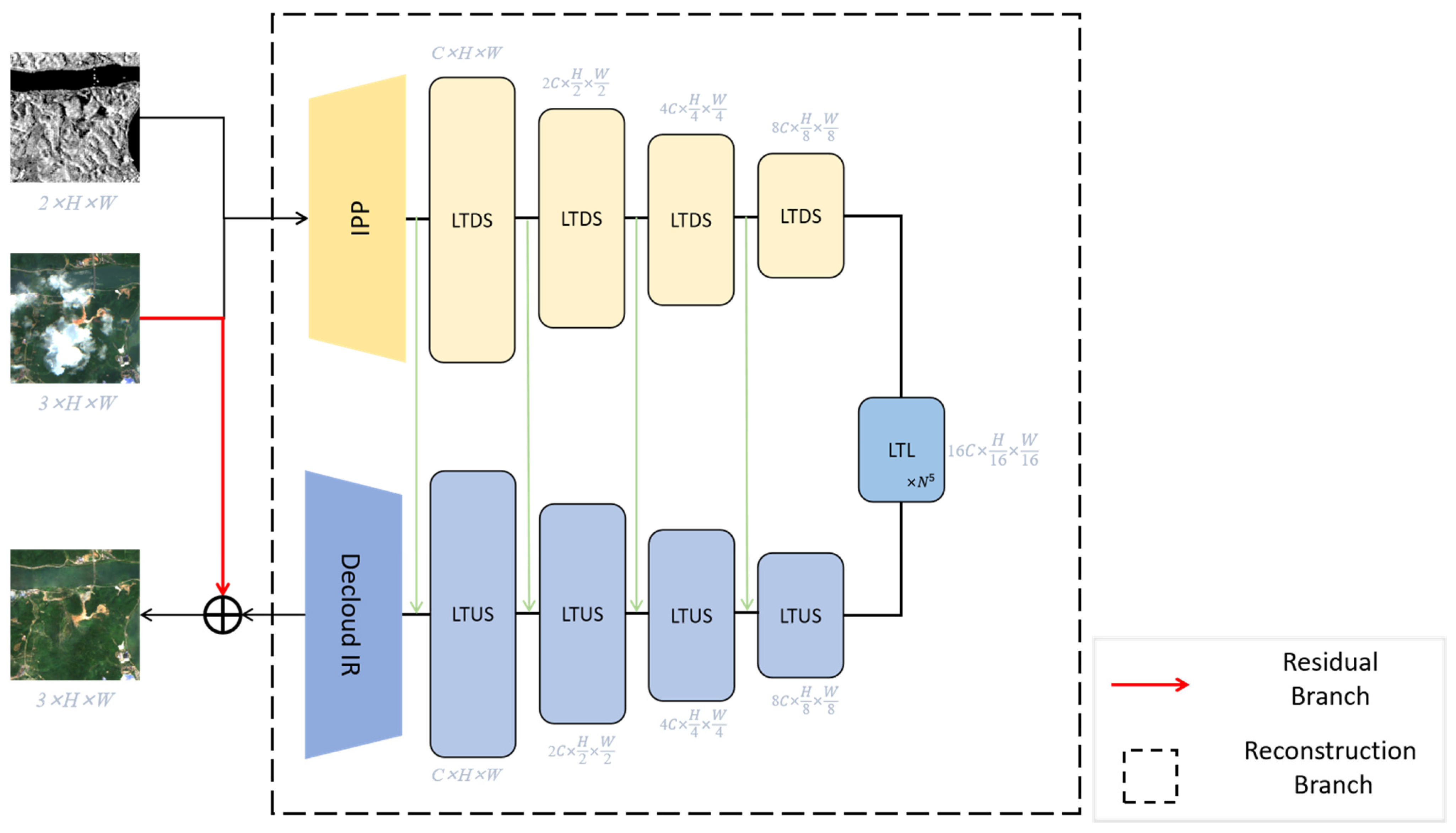
Given Transformer’s excellent performance and successful application in the field of image restoration, this work introduces it into a SAR-based remote sensing image cloud removal method in an attempt to tackle the problems and limitations of current cloud removal approaches. In this paper, we propose a Transformer-based cloud removal model called Former-CR. The network expands the input channel, allowing SAR images and RGB images to be input simultaneously to improve the authenticity of the reconstructed information and the overall cloud removal effect. Figure 1 shows the overall cloud removal process. The SAR image provides real structure information and texture information for the cloudy area, while the cloudless area of the RGB image can guide the color reconstruction. Our model introduces an enhanced Transformer module called Lewin (Locally-enhanced Window) Transformer block [38] to construct our model, which can extract and fuse the global–local information of the SAR image and the RGB image, so that the color, tone, texture, and structure information of the reconstructed area and the cloud-free area maintain global consistency. Specifically, Former-CR contains a residual branch and a reconstruction branch. The residual branch uses the residual connection to completely retain the cloud-free region information of the cloud RGB image, while the reconstruction branch meticulously designs a set of Lewin-Transformer block combinations to recover the cloud occlusion region information from the SAR and RGB images. Finally, the images of the two branches are merged to generate a predicted cloudless RGB image. The Transformer-based module group in the reconstruction branch brings superior performance, but its fixed number of input and output channels also causes the network to lose some flexibility. In order to better process remote sensing images and increase the scalability of the network, we designed an image preprocessor (IPP) to deal with multichannel input of the SAR and RGB images. Additionally, we propose a decloud image restorer (Decloud-IR) with channel attention mechanism to recover three-channel RGB images from the high-dimensional feature maps output by the Transformer-based module group, fully considering the contribution of different channels in the feature maps to generate remote sensing images. It is worth mentioning that both IPP and Decloud-IR allow for simple changes to the number of input and output channels. Their integration with the Transformer module set enables the feature reconstruction branch to balance performance and scalability. In addition, we built a new loss function to supervise the training model in order to improve the visual impression of the image, the overall structure, and the local details. In summary, the main contributions of this paper are summarized as follows:
  • We designed a Transformer-based multisource image cloud removal model, Former-CR, to recover cloudless optical images directly from SAR and cloudy optical images. It combines the reliable texture and structure information of the SAR image and the color information of the cloud-free area of the optical image, so as to reconstruct the cloud-free image with global consistency.
  • We designed IPP and Decloud-IR. IPP can improve the flexibility of model input and extract shallow features, while Decloud-IR is able to improve the output flexibility of our model and better map the feature to the output image space. The two increase the cloud removal model’s processing capacity for remote sensing images, as well as its flexibility and scalability.
  • In order to improve the image structural similarity, visual interpretability, and global consistency, a loss function that can comprehensively consider the above factors is proposed as the optimization objective of our model. The superiority of our loss function in cloud removal is extensively verified by ablation experiments.
In Section 2, we review the current work on thick cloud removal.
The structure of this paper is as follows: In Section 2, we review the current work on thick cloud removal. In Section 3, the method is introduced in detail. In Section 4, we introduce the experimental process and results to prove the effectiveness and superiority of the method. Conclusions, discussions, and future work are presented in Section 5.

2. Related Work

Satellites are being launched into space at an increasing rate to monitor the Earth’s surface. They are split into two categories based on the distinct functioning principles of the sensors: active remote sensing and passive remote sensing. Distinct types of images may have a diverse expression of ground objects, but they are all different expressions of the same ground; therefore, there are tight internal links between them. Currently, remote sensing optical images, as the most widely used images, suffer badly from cloud cover. As an active remote sensing sensor, SAR can observe the ground under any weather condition and obtain cloud-free images by virtue of its ability to resist cloud interference, which fundamentally solves the problem of information loss on optical images. In recent years, the SAR-based optical thick cloud removal method has become the emphasis of research.
Hoan et al. [28] and Eckardt et al. [29] use DN (Digital number) of SAR as an indicator to find the repair pixel, but they did not directly employ any SAR image information at all during information reconstruction, resulting in a significant waste of SAR image data. Bermudez et al. [30] used cGAN to transfer SAR images into optical images to replace cloudy optical images; the information of the cloudless image is 100% from the SAR image, which means that this method completely ignores the information of the cloudless area. The two methods mentioned above cause a significant waste of input photos. Whether using SAR information alone or using optical image information alone, the quality of cloud removal images cannot be further improved. The key issue of the multisource image cloud removal approach based on SAR images is how to fully utilize their unique advantages and functional fusion. In recent years, some scholars have explored the cloud removal method of SAR–optical image fusion. Grohnfeldt et al. [31] realized the cloud removal method of SAR image and multispectral image fusion for the first time by using cGAN, and verified the effectiveness of the cloud removal method of SAR–optical image fusion. The U-shaped encoding–decoding structure used in the model also takes into account the details of multiscale feature maps, which provides a feasible example for effective information fusion. Gao et al. [32] and Darbaghshahi et al. [33] used two GANs in series. The first GAN is responsible for the translation of SAR images to optical images, and the second GAN is responsible for the fusion of images for cloud removal. However, the learning of single-channel SAR images to multichannel optical images is an ill-posed problem [39], and the training and prediction of GANs are not stable enough. The way in which GANs are connected in series aggravates this instability. In order to overcome the problems caused by the use of the GAN correlation model in the above methods, Meraner et al. [34] used DNN to extract features from SAR images and cloudy optical images, and connected the feature map with the input cloudy optical image through the residual branch to obtain the predicted cloudless image. The residual branch can retain the information of the cloudless area to the greatest extent, and the feature extraction network focuses on the information reconstruction of the cloud area. Compared with the GAN-based cloud removal method, the cloud removal effect is not easily affected by the quality of the dataset, and can maintain stable prediction results under input data of different quality. This method provides a new idea for the fusion of SAR and optical images.
Cloud removal is essentially an image restoration process in which high-quality pictures are rebuilt from low-quality or information-deficient photos. Given its superior performance, the CNN-based image restoration approach has become mainstream. Dong et al. proposed SRCNN [40] for image super-resolution reconstruction, while Zhang et al. designed DnCNN [41] to eliminate noise from images. Since then, outstanding modules such as residual block and dense block have been successfully integrated into image restoration [42,43,44,45]. However, they generally suffer from two basic problems derived from the basic convolutional layer. First, CNN’s weight-sharing forces the model to use the same convolution when processing different regions. Second, the local perception property of CNN makes it difficult to capture long dependencies [37]. These problems restrict the application of CNN in the field of image restoration. Fang et al. noted the limitations of local convolution, designed a global–local fusion-based cloud removal (GLF-CR) method [46], introduced a self-attention mechanism to establish global dependency, and achieved a cloud removal effect beyond that of the existing methods. The success of GLF-CR proves the importance of global content information in remote sensing cloud removal tasks.
Transformer has shown remarkable performance in natural language processing (NLP) since it was proposed in 2017, which has also inspired computer vision researchers. ViT [47] pioneered the segmentation and serialization of images, so that the structure based on Transformer is no longer limited to text input and can be extended to image input. Different from CNN, the network structure based on Transformer captures the long-term dependency in the data through self-attention. Transformer has a natural advantage in solving tasks that require global information. IPT [36] was the first model to introduce Transformer into low-level vision tasks. It adapts to different tasks by fine-tuning the pretrained model. Based on Swin-Transformer [48], Swin-IR [37] improves it to complete various image restoration tasks, such as image super-resolution and rain removal. Although these models have achieved amazing results, their huge parameters and the extreme computation cost limit their in-depth study and application. In order to improve the performance of Transformer and reduce its computation cost, UFormer designed the Lewin Transformer module [38], which greatly reduces the parameters of the model through window-based multihead self-attention (W-MSA), and introduces convolutional layers to increase the ability of local feature extraction for Transformer. UFormer surpasses its predecessors with its smaller model volume, and also provides a more feasible and reliable solution for Transformer-based image restoration tasks.
Inspired by the above SAR-based optical image thick cloud removal methods and the application of Transformer in the field of image restoration, this paper attempts to use a Transformer-based module to fuse SAR and optical images for cloud removal.

3. Materials and Methods

Our model contains two crucial branches: the residual branch and the reconstruction branch. The residual branch copies and retains an input RGB cloudy image, waiting to be combined with the output of the reconstruction branch. The reconstruction branch has three steps: preprocessing, encoding–decoding, and image restoration. In the first step, shallow features of multisource images are extracted and mapped to the shape specified in the coding stage. The encoding–decoding part is a U-shaped structure, and shallow features obtained after preprocessing first enter the encoding stage to obtain high-dimensional features. The high-dimensional features are decoded to obtain a reconstructed feature map with the same shape as that of the input in the encoding stage. In the image restoration stage, a mapping is established to ensure that the output of the reconstruction branch is consistent with the form of the RGB image. To create a forecasted cloudless image, the final reconstructed image is merged with the RGB input image through the residual branch. The overall network structure of Former-CR is shown in Figure 2.

3.1. Reconstruction Branch

The three steps of the reconstruction branch are completed by IPP, encoder–decoder, and Decloud-IR, respectively. The first two are responsible for shallow feature extraction and deep feature reconstruction, while the image restorer converts the feature map space to the output image space.

3.1.1. Overall Pipeline

Given a SAR image I s a r   2 × h × w , with h and w being the height and width of the maps, and a cloudy RGB image I R G B   3 × h × w as input to the network, they first come to IPP, which is mainly composed of concatenation, convolution layer, and activation layer. It concatenates the input images to obtain I i n   5 × h × w , and a 3 × 3 convolution C o n v 3 is responsible for feature extraction. The convolution layer is good at early visual processing, leading to more stable optimization and better results [49]. In the last step, after the activation of LeakyReLU comes the output of the initial feature F i n i t   C × h × w . IPP can accept input from any number of channels and map it to a unified channel dimension C. Therefore, the design of IPP enables the network to receive multichannel input for different tasks, giving the model great flexibility and scalability. C represents the initial feature number of deep feature extraction, and multihead self-attention (MSA) uses the corresponding number of heads according to the number of feature channels. The larger C denotes a greater capacity for processing features, whereas the smaller C effectively reduces model volume. The formulaic expression of IPP is as follows:
I i n = C o n c a t . I S A R , I R G B
F i n i t = L e a k y R e L U C o n v 3 I i n
The encoder–decoder receives the shallow feature F i n i t to extract deep features. As shown in the reconstruction branch in Figure 2, the encoder contains four Lewin Transformer and Down-Sample (LTDS) blocks for feature extraction and down-sampling in 4 stages. Each LTDS includes N i Lewin Transformer layer (LTL), i = 1 ,   2 ,   3 ,   4 . The size of the feature map and the number of channels is unchanged with LTL. The down-sampling layer at the end of LTDS can shrink the size of the feature map by doubling the number of channels, halving the height and width, respectively. Each step’s feature maps are duplicated, stored, and then used as inputs for the following stage of coding.
A bottleneck stage with N 5 LTL is added after the encoder. At this stage, after multilevel encoding by the encoder, the collective of the Transformer captures a long-term dependency on feature maps of different sizes. The bottleneck layer performs the final feature extraction on the feature map. Due to the small size of the feature map received by the bottleneck layer, the global dependency can be learned through self-attention. The feature map size and number of channels are not modified at this stage.
Symmetrically, the decoder also contains four stages of decoding. According to the order of feature maps from small to large during decoding, each Lewin Transformer and Up-Sample block (LTUS) has N i   i = 4 ,   3 ,   2 ,   1 LTL and one up-sampling layer. Each step of decoding will produce a feature map with its height and width doubled, its number of channels cut in half, and it will be connected to the correspondingly sized feature map stored during coding using skip connection to conduct feature fusion before moving on to the next level of decoding. Finally, the decoder outputs a depth reconstruction feature map F d e e p   C × h × w with the same size and number of channels as F i n i t .
The value range of the target cloudless RGB image I t a r g e t   3 × h × w is [0, 1]. Compared with I t a r g e t , F d e e p usually has a different number of channels and a different range, so it is necessary to learn a mapping from feature space to image space. We use Decloud-IR to complete the learning process and obtain the restored image I R e c o n s t r   3 × h × w for final fusion.

3.1.2. Lewin Transformer and Sample

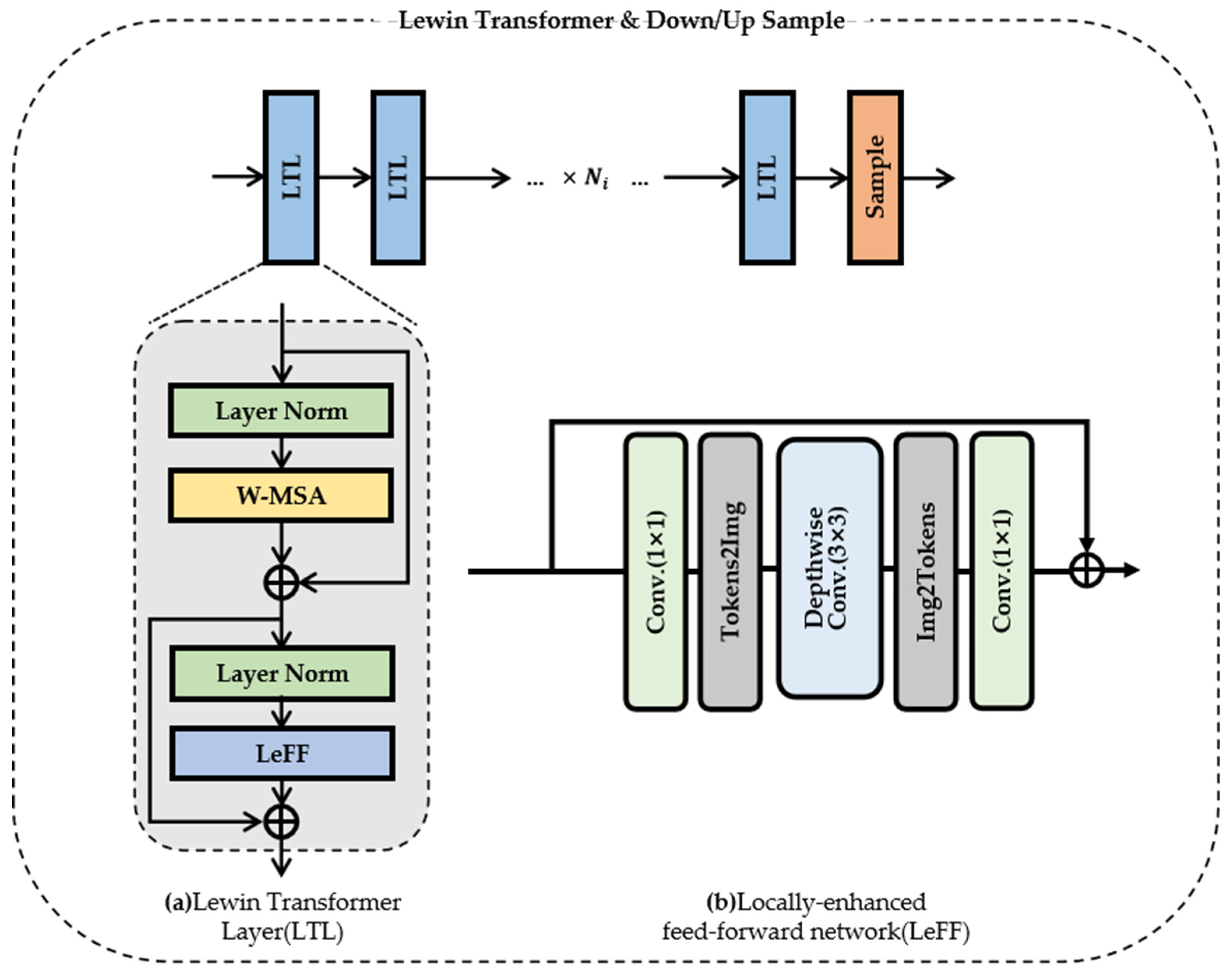
To complete feature extraction and adjust the dimension of the feature map, we utilize a combo of LTL and sampling layers in both the encoding and decoding phases. The structure is shown in Figure 3. It is further subdivided into LTDS and LTUS depending on the sample layer employed. To accomplish down-sampling in LTDS, a convolutional layer with a size of 4 × 4 and a stride of 2 is applied. To perform up-sampling in LTUS, a transposed convolutional layer with a size of 2 × 2 and a stride of 2 is applied. The core component in LTDS and LTUS is LTL, which is an improved form of the standard Transformer. There are two major obstacles to using Transformer for image restoration. First, the conventional Transformer design computes self-attention globally over all tokens, contributing to quadruple the computation cost with respect to the token count. It does not work to apply global self-attention on high-resolution feature maps. Second, local context information is critical for image restoration since the neighborhood of a damaged pixel may potentially provide necessary information for recovering. Nevertheless, it had been indicated in [50,51] that Transformer suffers from difficulty in accessing context information.
Lewin Transformer block provides a successful solution to those problem, and the Lewin Transformer architecture is shown in Figure 3a [38]. The locally-enhanced feed-forward network (LeFF) uses convolution to collect relevant local context information, while window-based multihead self-attention (W-MSA) executes self-attention in non-overlapping local windows to capture long-term dependency, considerably reducing the computational cost.
Given a 2D feature map X   C × H × W , firstly, X is divided into H W M 2 non-overlapping windows of M × M size, and then the features in window j are transformed into features X j   M 2 × C , j = 1 , 2 , .. , H W M 2 , by flatten and transpose. W-MSA applies self-attention in units of the characteristics of each window. For each local window feature X j , query, key, and value matrices Q, K, and V are calculated as follows:
Q = X j P Q , K = X j P K , V = X j P V
P Q , P K , and P V are the projection matrices of Q, K, and V. In general, we have Q, K, and V   M 2 × C . Therefore, the attention matrix calculated using the self-attention mechanism in the local window is as follows:
A t t e n t i o n Q , K , V = S o f t M a x Q K T d + B V
where B is learnable relative positional encoding. We execute k attention functions in parallel to obtain an MSA.
LeFF introduces a depth-wise convolutional block into the Transformer-based module. As shown in Figure 3b [38], LeFF first performs a linear projection layer to each token to expand its feature dimension. Then, each token is reshaped as a two-dimensional feature map for 3 × 3 deepwise convolution to capture local context information. The channel is then shrunk through another linear layer to match the dimension of the input channel after the feature is flattened to the initial token size. GELU [52] is used as the activation function after the above operations.

3.1.3. Decloud-IR

In the process of feature extraction, the value range of each layer of the feature map is different due to the different activation functions used, and the number of channels ( C ) of the obtained depth reconstruction feature map F d e e p   C × h × w is also different from that of the target image. In order to normalize the value range of the depth feature F d e e p and transform the dimension to the same dimension as that of the target optical image to facilitate the final residual connection, Decloud-IR was designed to complete the transformation process. The Decloud-IR accepts a feature map with channel C , and the output can be extended to any dimension according to the requirements of different tasks, thereby increasing the output flexibility of the entire network and the scalability of tasks.
As shown in Figure 4, Decloud-IR consists of a squeeze-and-excitation (SE) [53] module, a 3 × 3 convolution, and a sigmoid activation function. The SE module can learn the emphasis of different channels and has been widely used in image denoising, image super-resolution, and other low-level vision tasks. The 3 × 3 convolution transforms the feature map to the same shape as the target image, and introduces the inductive bias of the convolution operation into the Transformer-based module. Finally, the sigmoid function transforms the value of the feature map in the [0, 1] interval and outputs. The process for obtaining the I R e c o n s t r . is expressed as:
I R e c o n s t r . = s i g m o i d C o n v 3 S E F d e e p

3.2. Residual Branch

As a classic model in deep learning, ResNet [54] not only enables neural networks to design deeper layers but it also enhances model performance without introducing additional parameters. Inspired by ResNet and DSen2-CR [34], we designed a simple but powerful residual branch, which can be of considerable use in the following ways:
  • Cloud-free area information retention: The input cloud optical image is retained by the residual branch, which maximizes the reproduction of cloud-free area information at output, reducing contamination and changes to information outside the non-cloud occlusion area during information reconstruction. This is the largest contribution of the residual branch.
  • Accelerate model convergence: The residual connection before the output cloudless image can reduce the difference between the predicted image and the target image. Under the constraint of the loss function, the smaller the loss of the predicted image compared with the objective function, the faster the model converges.
  • Prediction stability: In the case of data input partially occluded by large areas of thick clouds, there is less effective information left in the optical image. The residual connection can at least save information about areas without clouds if it is impossible to retrieve high-quality cloud information throughout the reconstruction phase. Therefore, even under the worst-case scenarios, the model’s output is not much poorer than the input cloud image. Our model with residual connection offers significant benefits in producing steady outcomes when compared to the unstable prediction or inaccurate prediction of CGAN-based approaches in the situation of bad data quality.
In addition to the residual branch, we also used a similar skill in the reconstruction branch. Skip connection, as shown in the green line in Figure 2, can also be regarded as a residual connection. It can give full play to the advantages of residual connection, and is conducive to the pixel-level information fusion between the encoded feature map information and the decoded feature map.

3.3. Loss Function

The classic loss function L1 pixel-by-pixel comparison information can intuitively and quickly evaluate the quality of the generated image, thus effectively constraining the image quality. The L1 loss function is defined as follows:
L o s s L 1 = y p y g t
However, since cloud optical pictures, cloudless optical images, and SAR images are not acquired simultaneously when we use the dataset created by real images, we cannot ensure that the ground object information is entirely consistent. Additionally, the information, such as color and brightness of the two images, will be more or less altered as a result of the thick clouds that exist between the optical image with clouds and the optical image without clouds. Technically we are unable to acquire the ground truth cloudless image that corresponds to the cloudy optical image. Consequently, using solely the L1 distance to evaluate the quality of the produced picture is a little bit too stringent, and paying too much attention to detail information leads to the neglect of the overall reconstruction quality of the image.
In order to address the above problems and bring the predicted image more in line with human perceptual similarity judgments, we introduced learned perceptual image patch similarity (LPIPS) [55] to improve the overall image quality. LPIPS can map the predicted image and the real image to the same dimension in the same way, and prioritize the perceptual similarity between them. Formula (7) depicts the definition of LPIPS:
L o s s l p i p s = l 1 H l W l h , w w l y h w l y 0 h w l 2 2
where y l and y 0 l represent the real data and the generated data, respectively. The L2 distance is calculated between each corresponding channel, and the weighted sum is obtained in the channel dimension, and w l is the channel weight.
Our last loss function is the weighted sum of the previous two. The loss function is shown below.
L o s s = L o s s l p i p s + L o s s L 1

3.4. Metric

To evaluate the quality of the reconstructed image, we used several popular pixel-level reconstruction quality evaluation indicators, structural similarity (SSIM), mean absolute error (MAE), and peak signal-to-noise ratio (PSNR), as our evaluation criteria.

3.4.1. SSIM

SSIM is an index assessment approach that measures how similar two pictures are to one another, which is determined by brightness, contrast, and picture structure. The formulae are, correspondingly, Equations (9)–(11):
l X , Y = 2 μ X μ Y + C 1 μ X 2 + μ Y 2 + C 1
c X , Y = 2 σ X σ Y + C 2 σ X 2 + σ Y 2 + C 2
s X , Y = σ X Y + C 3 σ X σ Y + C 3
C 1 , C 2 , C 3 are constants to avoid dividing by zeros. μ and σ are the mean and variance of the image, and σ X Y is the covariance of image X and Y. Therefore, the formula of SSIM is as follow:
S S I M = l X , Y c X , Y s X , Y
The value range of SSIM is between 0 and 1, and the larger the value is, the more similar the value between the two images is. If the value is 1, the two images are identical.

3.4.2. PSNR

PSNR is the most widely used objective measurement method to evaluate image quality. Its formula is as follow:
P S N R = 10 log 10 2 n 1 2 M S E
Here, 2 n 1 is the maximum possible pixel value of the image. The general pixel is 8 bits, which means the pixels are represented using 8 bits per sample. Remote sensing images usually have a higher number of n. MSE is the mean square error between image X and image Y, and the calculation method is:
M S E = 1 H × W i = 1 H j = 1 W X i , j Y i , j 2
The value range of PSNR is generally 20~40. The larger the value is, the closer the distance between the predicted image and the real ground image is, and the better the prediction quality is.

3.4.3. MAE

MAE is a measure of the error between pairs of observations representing the same phenomenon. MAE is calculated as the sum of absolute errors divided by the sample size. The specific calculation process is shown in Formula (15):
M A E = i = 1 n y i x i n

4. Results

4.1. Dataset

The data used in this paper are from the large-scale dataset SEN12MS-CR [56]. The images of SEN12MS-CR are all from the Sentinel satellite images of the Copernicus project. The dataset covers the geographical and meteorological conditions of all continents, meteorology and seasons, with a total of 169 non-overlapping regions. The image size of each region is about 5200 × 4000 pixels, and the data are sliced according to the size of 256 × 256 and 50% spatial overlap. A total of 122,218 triple samples are generated. Each sample includes a Sentinel-1 dual-polarized (VV and VH) SAR image after ortho-correction and geographic registration, a Sentinel-2 cloudless multispectral image, and a Sentinel-2 cloud-covered multispectral image, where the acquisition time of the cloudless and cloud-covered images is close. The VV and VH polarization images of the SAR image are cut to values [−25, 0] and [−32.5, 0], respectively, and rescaled to the range [0, 1]. The bands of all optical images are cut to values [0, 10,000] and then normalized to the range of [0, 1].
Given the high computational cost of the Transformer model and our experimental conditions, we chose the summer pictures of the SEN12MS-CR dataset for training in order to control the training time. The selected dataset contains 34,361 pairs of samples. We only used VH polarized SAR data and RGB band optical images as input during training. All data were divided into training set, validation set, and test set according to the proportion of 85:10:5, that is, the number of images in the training set, validation set, and test set was 29,207, 3436, and 1718, respectively. The dataset was divided in a random manner.

4.2. Training Setting

The proposed Former-CR model was trained on 2 NVIDIA 3090 GPUs. We used the AdamW optimizer [57] to train our model with momentum terms of (0.9, 0.999) and a weight decay of 0.02. The initial learning rate (lr) was 0.0005, and it reduced 0.5 times every 50 epoch. The window size was set to 8 × 8 in all LeWin Transformer blocks. By default, the number of stages was the same for the encoder and decoder, and was set to 4. The number of repetitions of LTL in each layer of encoder and decoder was N 1 = N 2 = N 3 = N 4 = 2 , N 5 = 4 , and the number of channels starting the encoder was C = 16 .
The input of our network was SAR and cloud RGB images, respectively. The default shapes were as follows: the SAR image was 2 × 256 × 256, and the cloud RGB image was 3 × 256 × 256. The shape of the output predicted cloudless RGB image was 3 × 256 × 256.
Training for our model took about 45 h.

4.3. Experient Result

We compared our method with the state-of-the-art cloud removal methods, including SAR-Opt-cGAN, proposed by Grohnfeldt et al. [31], DSen2-CR, proposed by Meraner et al., and GLF-CR, proposed by Xu et al. All those methods use SAR images and multispectral images as input for cloud removal. As the first cGAN architecture fusing SAR and optical MS data to remove cloud [31], SAR-Opt-cGAN’s network architecture is mostly based on U-Net [58]. The comparison between our model and SAR-Opt-cGAN can prove how far we have developed in cloud removal research. DSen2-CR uses a well-designed DNN, which is extended from EDSR [59], with some improvements. Considering the important role of global information, GLF-CR, in particular, has two parallel backbones designed for optical and SAR image representation learning, with SAR characteristics applied hierarchically to correct for information loss. The above-mentioned DSEN2-CR and GLF-CR represent the SOTA of the DNN method and the method using the self-attention mechanism, respectively. The Former-CR proposed in this paper is a Transformer-based model for cloud removal.
Although Transformer has excellent performance, it has been criticized for its huge computational cost. Considering that no bands except RGB in multispectral images can provide effective information for true-color visual images, and the input of multispectral images will bring large computational burden to the training of the model, we only used the images of three bands (RGB) for cloud removal. We constantly utilized dual-polarization SAR images and RGB images as input for training and testing the three models mentioned above as well as our model in order to compare model performance objectively.
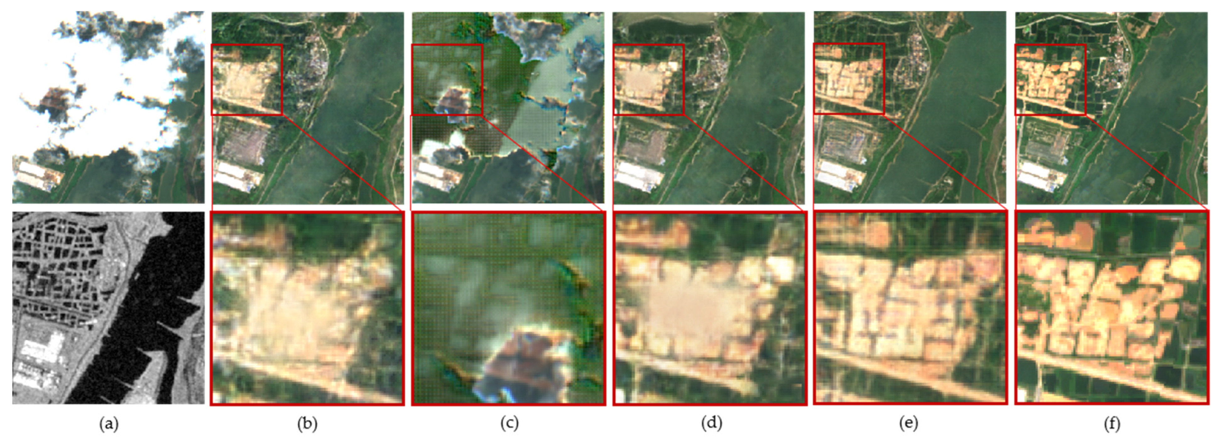
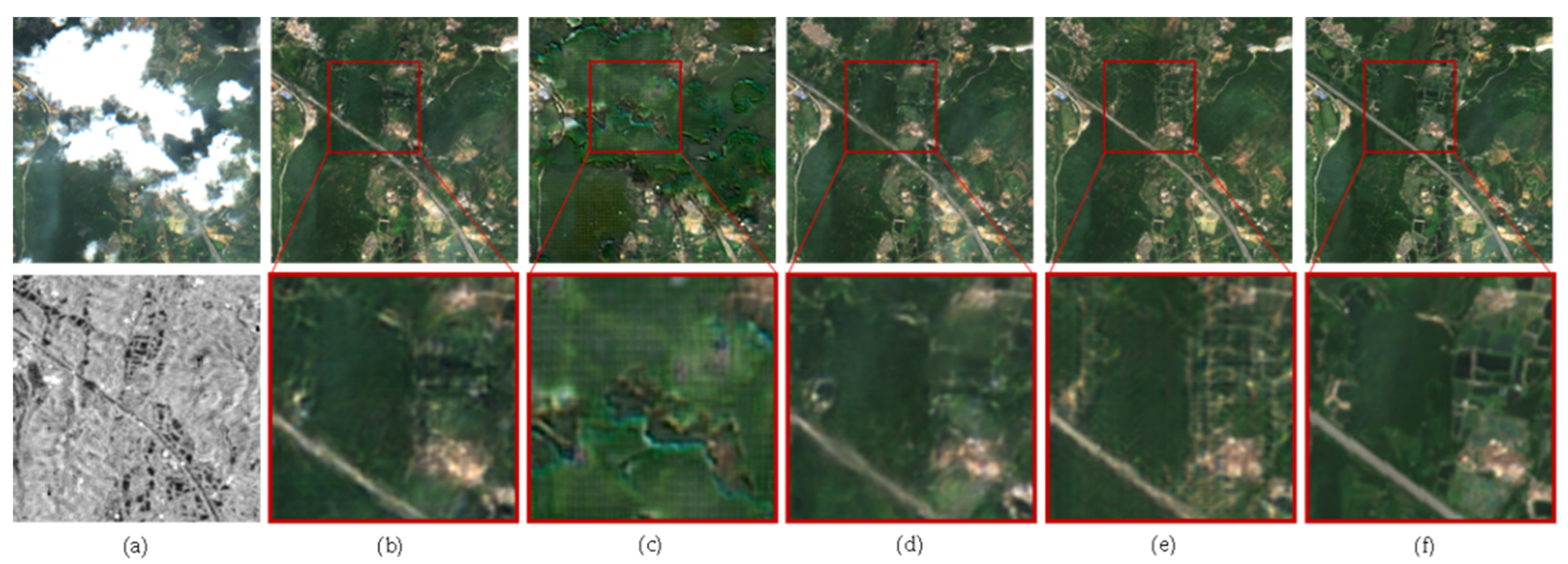
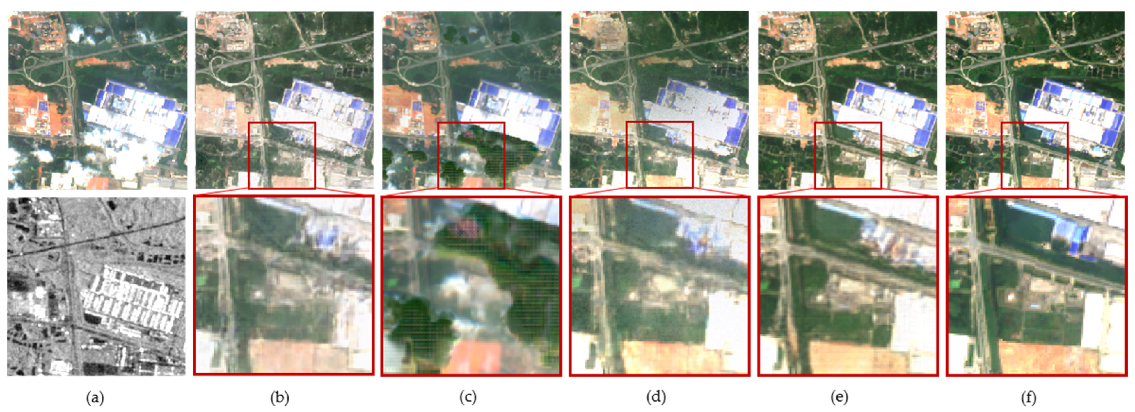
The four scenes we selected include many types of ground objects such as towns, rivers, farmland, roads, and mountains. At the same time, the area of thick cloud coverage in the scene is also different. The area of cloud coverage is arranged in order from large to small in the four scenes. We analyze the advantages and disadvantages of our method and other cloud removal methods by displaying and analyzing the overall and details of the predicted cloud removal images.
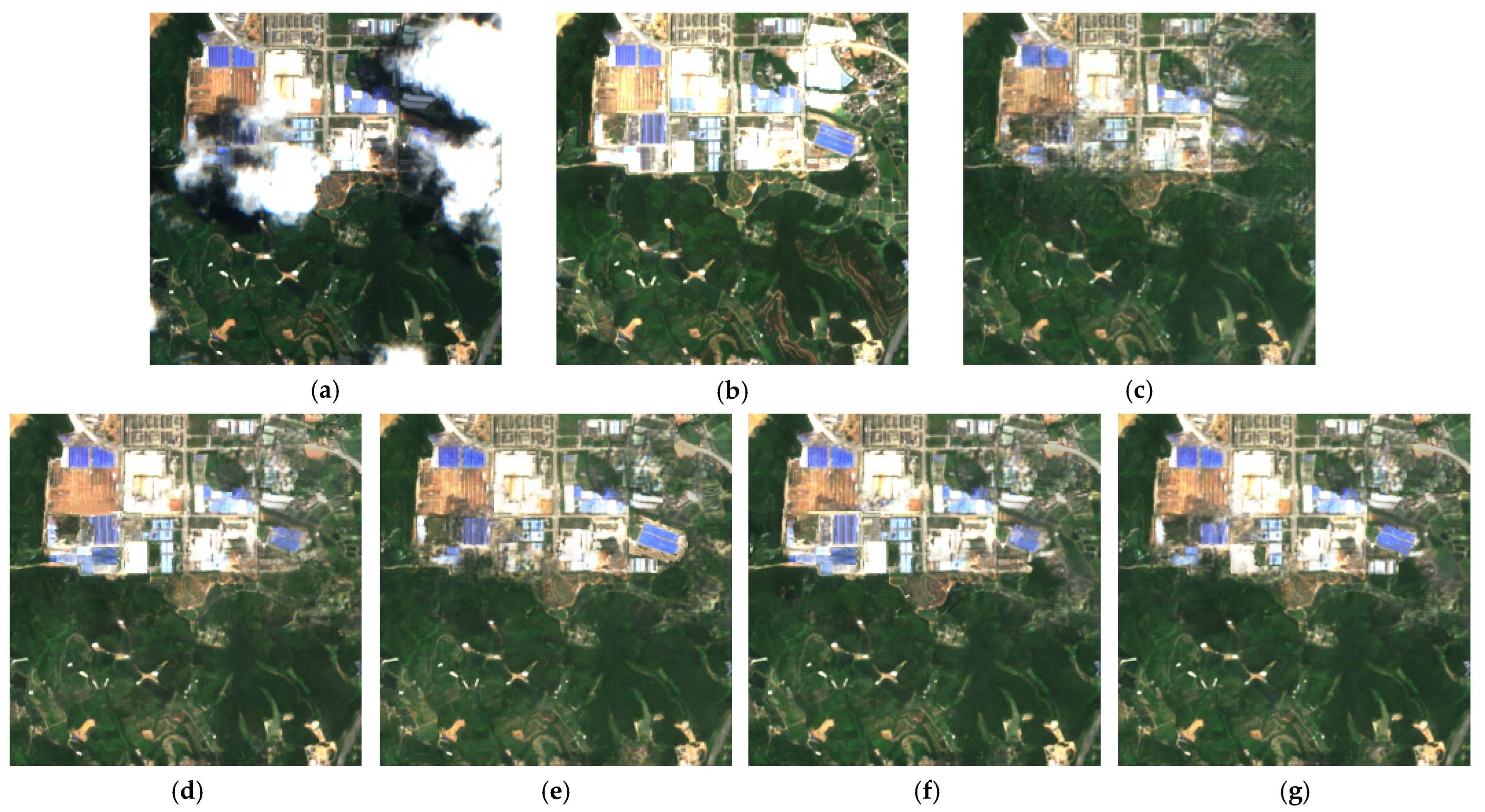
The overall visual effect of the image is shown in the odd rows in Figure 5, Figure 6, Figure 7 and Figure 8. The image predicted by DSen2-CR of four scenarios can basically locate where there are dense clouds and perform some processing, and the residual structure in the network helps the predicted image to retain the information of the cloud-free area completely. However, the DSen2-CR image’s rebuilt region lacks sufficient texture and structure, and the hue and tone are inconsistent with that of the cloud-free area, making it challenging to visually extract information from the reconstructed area. The images predicted by SAR-Opt-cGAN, GLF-CR, and our method show good results in terms of overall clarity, color restoration, and structural similarity. For SAR images with strong structural information, such as roads, coastlines, ridges, and contours, SAR-Opt-cGAN, GLF-CR, and our method can have a great restoration effect. Compared with GLF-CR and Former-CR that use global information, SAR-Opt-cGAN has a slightly inferior reconstruction effect, especially in some relatively dense and faintly blurred areas. In the fourth scene shown in Figure 8, although the thick cloud occlusion area is small, the entire image is covered by thin clouds, resulting in poor overall image clarity. SAR-Opt-cGAN successfully removes thick clouds, but the overall tone of the image predicted by the image is brighter and the contrast is not clear enough. Meanwhile, the characteristics of the thin-cloud-covering area and the cloudless area have altered a little from the original cloudy image. GLF-CR overcorrects the tone prediction of the image, and the overall image is dark, indicating that it is not strong against thin cloud interference. Compared with the above two methods, our method is superior in tone, contrast, and sharpness. It basically restores the color of the original image perfectly and maintains a high consistency.
Our model performs better than the other three models when analyzing the details of the rebuilt picture. For detailed comparison, the second row of images in Figure 5, Figure 6, Figure 7 and Figure 8 shows the enlargement of the same area in the reconstructed images by different methods. The DSen2-CR method failed to recover effective details in all four scenarios. SAR-Opt-cGAN performed poorly in detail clarity. Even if the obvious structural information in SAR is well utilized, there is no obvious boundary between different objects in the RGB image, which also leads to local blur. GLF-CR performed better in determining the contour and boundary of the ground object, but the drawback is that the ground object’s information was not properly recovered. Take the prediction of bare soil in Figure 5 as an example, although the whole bare soil area is completely restored, the block inside the bare soil is not obvious enough. In contrast, our method performed better, showing more detail regarding texture and structure. Our method obtained better information in all situations, not just the initial one. Even in the face of complex conditions, such as in the fourth scenario, our technique produced a remarkable stable reconstruction outcome.
The visual effects of the full images and the details show that our method produces a good cloud removal effect in mountain, city, or farmland scenes, which denotes it is universal for different scenes. In addition, despite diverse levels of cloud occlusion and variously complicated ground objects, our approach can retain the stability of the cloud removal effect. To our surprise, our method can maintain the stability of the cloud removal effect in the face of different degrees of cloud occlusion.
We randomly divided the test set into ten batches, and calculated the average value of the indicators for each batch. Table 1 displays the SSIM, PSNR, and MAE mean and floating range for the test set. In the quantitative results analysis, our method achieved the best results. The SSIM index can reflect the degree of global structure information recovery. SAR-Opt-cGAN and DSen2-CR are significantly lower than GLF-CR and our proposed method in SSIM index because they are unaware of the global content information. Our method adopts the Lewin Transformer module, which can take into account both global content information and local content information. At the same time, SAR image information and RGB image information are encoded together in the coding stage. Compared with the GLF-CR method, which extracts the features of SAR image information and RGB image information, respectively, and then merges them, our method implicitly completes the fusion of global–local information and SAR-RGB information in the coding process, and automatically learns better fusion methods with the learning ability of Transformer. According to the data shown in Table 1, our approach indeed slightly outperforms the GLF-CR in terms of metrics, and has the smallest fluctuation.

4.4. Loss Function Ablation Experiment

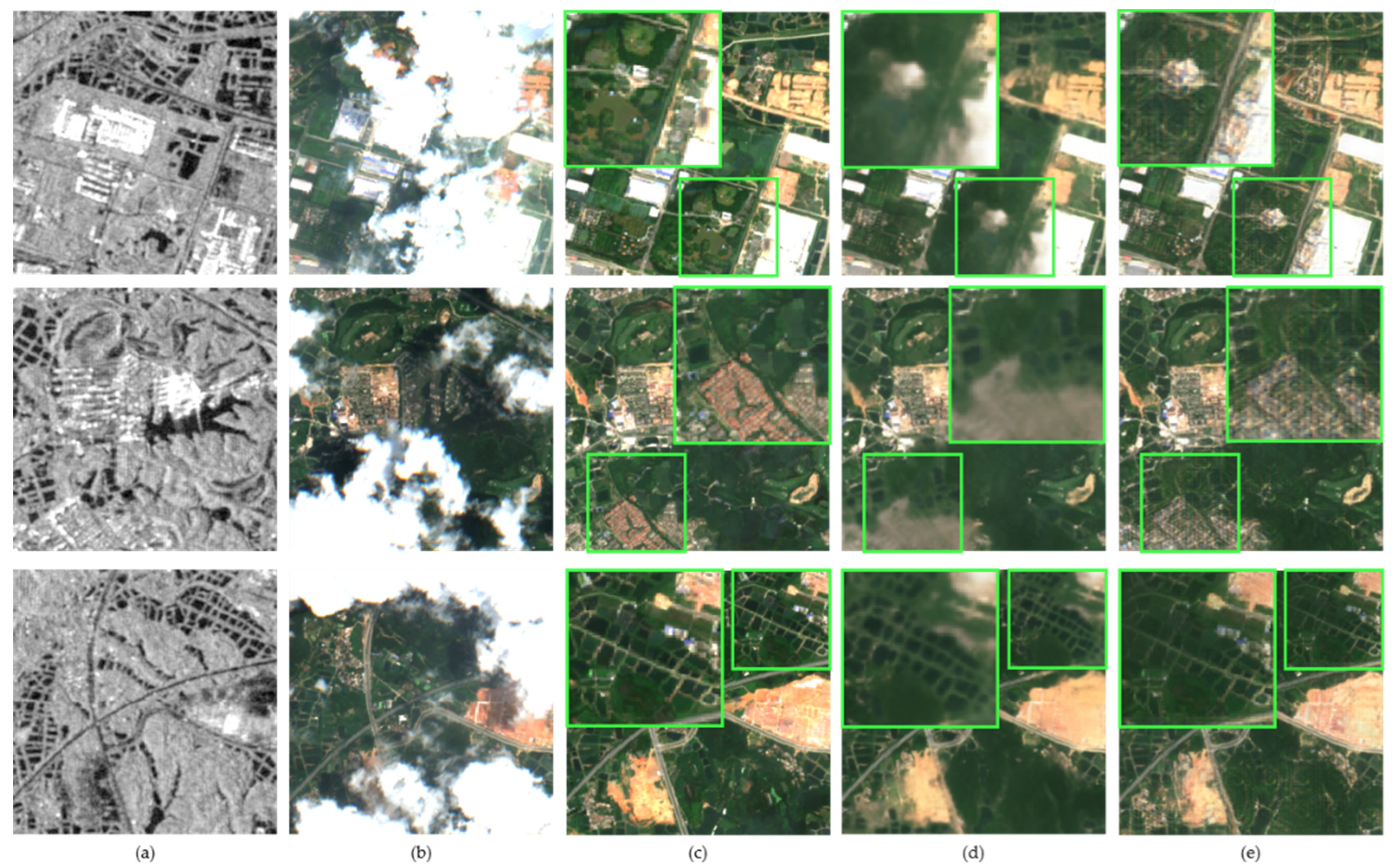
In order to explore the effectiveness and superiority of the loss function proposed in our method, we conducted ablation experiments involving loss function. We used the Former-CR model to train under the condition that the training dataset and parameters were exactly the same as those in the former experiment. The loss function was the only variable, which includes the L1 loss and the loss function proposed in this paper. Figure 9 shows the effect of cloud removal by different loss functions in three scenarios. The L1 loss function is effective in guiding the reconstruction of information at the pixel level, and the recovered image pixels are similar, but texture and structural information are difficult to distinguish. As shown in the zoomed display of the green box area in Figure 9, the details are not clear enough. Our approach can reproduce most of the texture information in the larger region, and the overall clarity of the image is enhanced. The addition of LPIPS may certainly boost the visual impression of the picture, and the local reconstruction effect is also significantly enhanced, according to the results of the overall comparison.
Table 2 displays the qualitative analysis of ablation experiments. We have an intuitive sense that the final L1 metric cloud be better improved upon by the L1 loss function. However, our loss outperforms L1 loss in terms of SSIM, PSNR, and even L1 measures. The reasonable combination of multiple loss functions means that the optimization direction of the image is constrained from multiple aspects. This counterintuitive phenomenon indicates that different loss functions will potentially promote each other, especially when our method can reconstruct a good enough image. In other words, an increase in the LPIPS index may cause the network to prioritize L1 distance optimization. Likewise, lowering the L1 index will accelerate the optimization of the LPIPS index.

4.5. Parameters Ablation Experiment

In the above experiments, our model achieved excellent results in visual effects and evaluation indicators. However, compared with some CNN-based methods, the computational power requirements and computational consumption of our model are difficult to control at a satisfactory level, which is often an important factor related to whether the method can be applied in practice. On the basis of keeping the overall framework of our model unchanged, adjusting the combination of hyperparameters for comparative experiments is a key way to explore model optimization.
The hyperparameters used in the model mainly include the initial learning rate (lr) and its decay parameters, optimizer and its parameters, number of LTL in each stage of encoder-decoder N i , and initial number of head C . In our model, the optimizer and its parameters do not change during training, while lr decays to the set minimum. Therefore, the former two usually only affect the speed of model optimization and hardly affect the final effect of the model. In the experiment, we used enough training cycles to weaken the influence of both. In addition to the above two, the hyperparameters that affect the performance of the model are mainly N i and C . To explore how these two hyperparameters affect the performance of our model, we set a series of representative parameter combinations for comparative experiments. The model’s performance was studied under different parameter combinations by comparing its visual effects, parameters, PSNR and SSIM. For the purpose of holding the variables unchanged and controlling the training time of each model, we used the same small-scale dataset for training. The dataset contains only 1500 sets of data, which was convenient for the rapid training and testing of the model. Except for N i and C , the remaining parameters are consistent with Section 4.2. Table 3 lists the specific parameters in each combination.
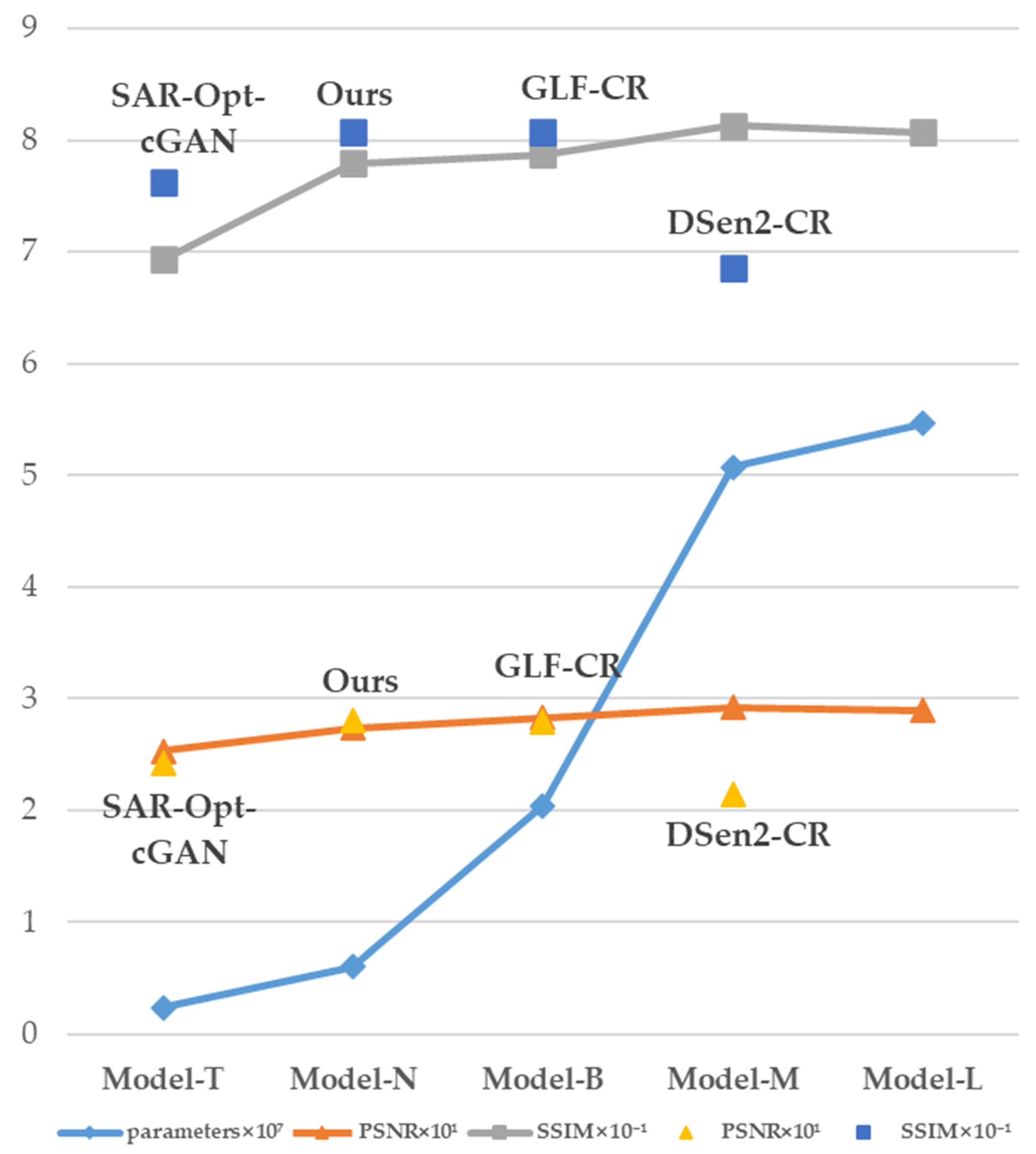
The indicators of different cloud removal models are shown in Figure 10. It can be clearly seen that with the increase of N and C , the parameters of the model increase sharply. When we reduce all the hyperparameters to 1, the number of parameters is the smallest, but it brings a significant decline in the index. Compared with previous experiments, it can only surpass DSen2-CR. After slightly increasing the depth of each encoder and decoder to the standard experimental parameters, the parameters of the model on each index are basically restored to the original level, meanwhile there is no increase in the number of exaggerated parameters. The comparison between the first two shows that our original parameter combination brings huge gains while taking into account the model volume. Comparing Model-N and Model-T, keeping C unchanged and continuing to increase the depth slightly improves the two indicators of SSIM and PSNR, but the number of model parameters quadruples, which cannot be ignored. Upgrading from Model-B to Model-L merely increases the number of C , and the performance remains unchanged, but the number of parameters has exploded. The above pairwise comparison is sufficient to show that the number of parameters can affect the performance of the model within a certain range, but blindly stacking the parameters does not bring a qualitative improvement to the model effect, but will damage the overall performance of the model in terms of training time and difficulty. The comparison between Model-M and Model-L shows that there is not much difference in the number of parameters and the total depth, but Model-M performs slightly better than Model-L does at the parameter level of 50 million. We speculate that this is owing to the model’s hierarchical depth architecture, which presents ideas for future network enhancement.
In addition, we also note that there is no significant difference in PSNR and SSIM whether we train our model on small datasets (Section 4.5) or large datasets (Section 4.3), which proves that our model can maintain a good performance with limited datasets.
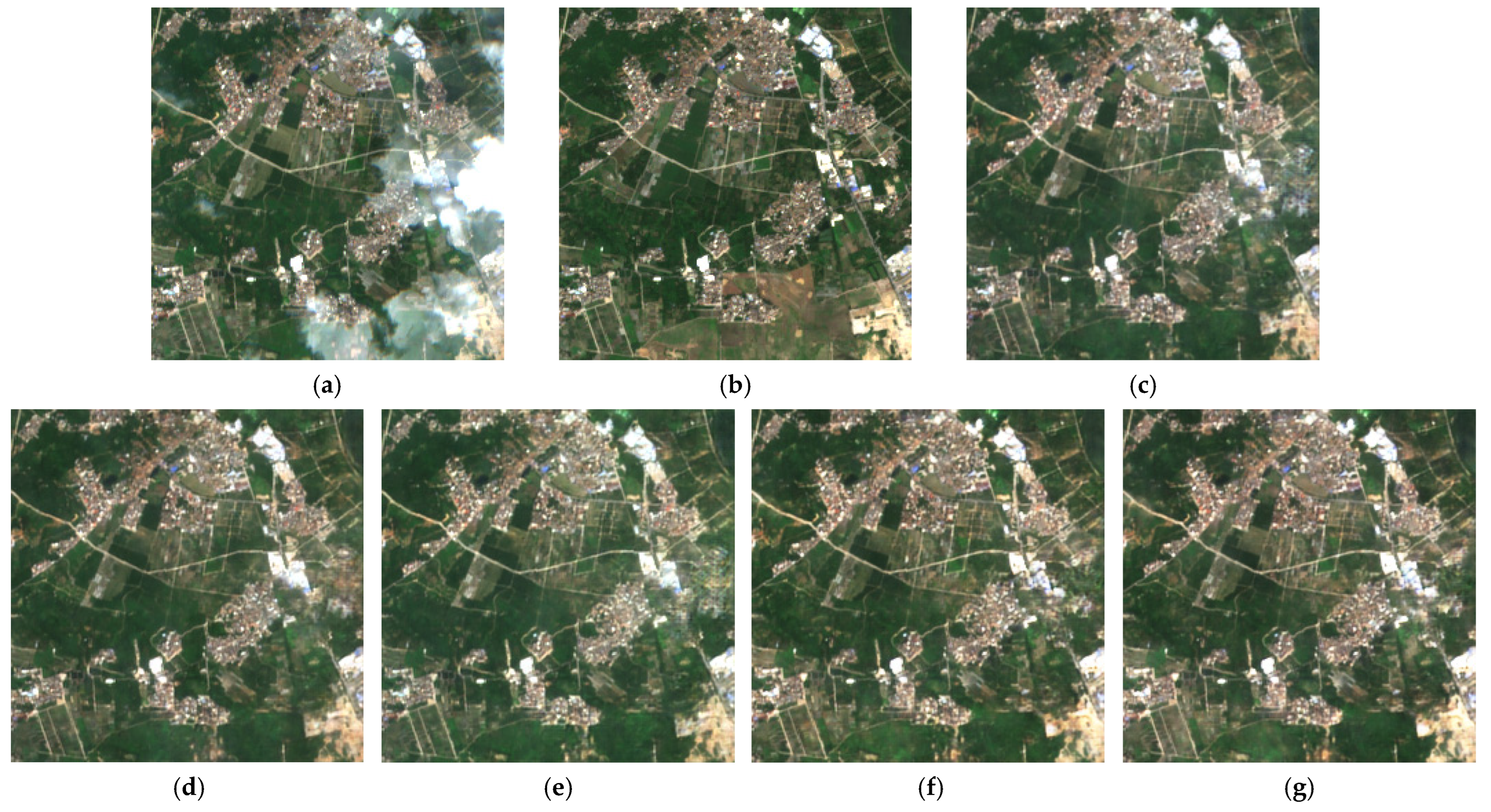
Figure 11 and Figure 12 show the cloud removal effects of different models. Compared with other models, Model-T is obviously inferior in the overall effect and texture effect of the image, which is consistent with its performance in the index. The visual effects of Model-N and Model-B are relatively close, indicating that the increase in the number of parameters does not bring equivalent returns to the cloud removal effect. The effects of Model-M and Model-L with large parameters are better in the detailed texture restoration of some regions, as shown in Figure 11.

5. Conclusions

In this paper, we introduce Transformer into a thick cloud removal task, and propose a Transformer-based global information fusion cloud removal method, Former-CR, which uses an SAR image and an RGB image as input to predict a cloudless RGB image. To design our model, we made extensive use of an innovative Transformer-based module called Lewin-Transformer, which integrates convolution into Transformer to provide Transformer-based network local information collection capabilities. Therefore, while reconstructing images, our method takes into account both global and local information, resulting in superior global consistency and color restoration in our predicted images. Furthermore, we created a novel loss function to increase the aesthetic effect and the detail reconstruction. We trained and evaluated the performance of our model using a real dataset from the open-source dataset SEN12MS-CR. The remarkable effect demonstrates the efficacy of our strategy. Compared with other fusion cloud removal methods based on the SAR image, our method performs better in both qualitative and quantitative evaluation, which proves the superiority of our method. Furthermore, we demonstrated that our proposed loss function works well in ablation experiments. To increase our model’s adaptability, we developed IPP and Decloud-IR to enable flexible input and output. The former allows our model to accept input from different dimensions and the latter produces output with the corresponding dimension of the target.
Limited by the huge computational power consumption of Transformer, it is difficult for our model to process input images with higher dimensions. Although the Lewin-Transformer module lowered computational power usage by applying self-attention on the window, it was far from sufficient to attain CNN levels. It is one of our regrets that we did not use more bands for experiments, but the high flexibility and scalability of Former-CR makes it convenient for us to conduct further research. A future research direction may be to try the fusion cloud removal experiment of hyperspectral (13-band) images and full-polarization (VV, VH, HH, HV) SAR images. In addition to attempting to tackle the current difficulties of a higher processing power, one of the most useful research paths concerns how to further compress the volume of Transformer-based modules and develop a more lightweight decloud model.

Author Contributions

Conceptualization, J.W.; methodology, S.H. and J.W.; validation, S.H. and J.W.; formal analysis, S.H. and J.W.; investigation, J.W. and S.H.; writing—original draft preparation, J.W., S.Z. and S.H.; writing—review and editing, J.W. and S.H.; supervision, J.W. and S.Z.; project administration, J.W. and S.Z.; funding acquisition, J.W. All authors have read and agreed to the published version of the manuscript.

Funding

This research was funded by Natural Science Foundation of China, grant number 42271367.

Acknowledgments

The authors would like to thank the editors and anonymous reviewers for their valuable comments and suggestions, as well as those researchers who make public codes and public datasets.

Conflicts of Interest

The authors declare no conflict of interest.

References

  1. Li, W.B.; Li, Y. Thick Cloud Removal with Optical and SAR Imagery via Convolutional-Mapping-Deconvolutional Network. IEEE Trans. Geosci. Remote Sens. 2020, 58, 2865–2879. [Google Scholar] [CrossRef]
  2. Rossi, R.E.; Dungan, J.L.; Beck, L.R. Kriging in the shadows: Geostatistical interpolation for remote sensing. Remote Sens. Environ. 1994, 49, 32–40. [Google Scholar] [CrossRef]
  3. Van der Meer, F. Remote-sensing image analysis and geostatistics. Int. J. Remote Sens. 2012, 33, 5644–5676. [Google Scholar] [CrossRef]
  4. Maalouf, A.; Carré, P.; Augereau, B.; Fernandez-Maloigne, C. A bandelet-based inpainting technique for clouds removal from remotely sensed images. IEEE Trans. Geosci. Remote Sens. 2009, 47, 2363–2371. [Google Scholar] [CrossRef]
  5. Cheng, Q.; Shen, H.; Zhang, L.; Zhang, L.; Peng, Z. Missing information reconstruction for single remote sensing images using structure-preserving global optimization. IEEE Signal Process. Lett. 2017, 24, 1163–1167. [Google Scholar] [CrossRef]
  6. Meng, F.; Yang, X.; Zhou, C.; Li, Z. A Sparse Dictionary Learning-Based Adaptive Patch Inpainting Method for Thick Clouds Removal from High-Spatial Resolution Remote Sensing Imagery. Sensors 2017, 17, 2130. [Google Scholar] [CrossRef] [Green Version]
  7. Zheng, J.; Liu, X.; Wang, X. Single Image Cloud Removal Using U-Net and Generative Adversarial Networks. IEEE Trans. Geosci. Remote Sens. 2021, 59, 6371–6385. [Google Scholar] [CrossRef]
  8. Lin, C.; Tsai, P.; Lai, K.; Chen, J. Cloud removal from multitemporal satellite images using information cloning. IEEE Trans. Geosci. Remote Sens. 2013, 51, 232–241. [Google Scholar] [CrossRef]
  9. Kalkan, K.; Maktav, M.D. A Cloud Removal Algorithm to Generate Cloud and Cloud Shadow Free Images Using Information Cloning. J. Indian Soc. Remote Sens. 2018, 46, 1255–1264. [Google Scholar] [CrossRef]
  10. Storey, J.; Scaramuzza, P.; Schmidt, G.; Barsi, J. Landsat 7 scan line corrector-off gap-filled product development. In Proceedings of the Pecora 16 Conference on Global Priorities in Land Remote Sensing, Sioux Falls, SD, USA, 23–27 October 2005. [Google Scholar]
  11. Zhang, X.; Qin, F.; Qin, Y. Study on the thick cloud removal method based on multi-temporal remote sensing images. In Proceedings of the 2010 International Conference on Multimedia Technology, Ningbo, China, 29–31 October 2010; IEEE: Piscataway, NJ, USA; pp. 1–3. [Google Scholar]
  12. Du, W.; Qin, Z.; Fan, J.; Gao, M.; Wang, F.; Abbasi, B. An efficient approach to remove thick cloud in VNIR bands of multi-temporal remote sensing images. Remote Sens. 2019, 11, 1284. [Google Scholar] [CrossRef] [Green Version]
  13. Zeng, C.; Long, D.; Shen, H.; Wu, P.; Cui, Y.; Hong, Y. A two-step framework for reconstructing remotely sensed land surface temperatures contaminated by cloud. ISPRS J. Photogramm. Remote Sens. 2018, 141, 30–45. [Google Scholar] [CrossRef]
  14. Li, Z.; Shen, H.; Cheng, Q.; Li, W.; Zhang, L. Thick cloud removal in high-resolution satellite images using stepwise radiometric adjustment and residual correction. Remote Sens. 2019, 11, 1925. [Google Scholar] [CrossRef] [Green Version]
  15. Cheng, Q.; Shen, H.; Zhang, L.; Yuan, Q.; Zeng, C. Cloud removal for remotely sensed images by similar pixel replacement guided with a spatio-temporal mrf model. ISPRS J. Photogramm. Remote Sens. 2014, 92, 54–68. [Google Scholar] [CrossRef]
  16. Lin, C.H.; Lai, K.H.; Chen, Z.B.; Chen, J.Y. Patch-based information reconstruction of cloud-contaminated multitemporal images. IEEE Trans. Geosci. Remote Sens. 2013, 52, 163–174. [Google Scholar] [CrossRef]
  17. Zhang, Y.; Wen, F.; Gao, Z.; Ling, X. A Coarse-to-Fine Framework for Cloud Removal in Remote Sensing Image Sequence. IEEE Trans. Geosci. Remote Sens. 2019, 57, 5963–5974. [Google Scholar] [CrossRef]
  18. Wen, F.; Zhang, Y.; Gao, Z.; Ling, X. Two-pass robust component analysis for cloud removal in satellite image sequence. IEEE Geosci. Remote Sens. Lett. 2018, 15, 1090–1094. [Google Scholar] [CrossRef]
  19. Li, X.; Shen, H.; Zhang, L.; Zhang, H.; Yuan, Q.; Yang, G. Recovering quantitative remote sensing products contaminated by thick clouds and shadows using multitemporal dictionary learning. IEEE Trans. Geosci. Remote Sens. 2014, 52, 7086–7098. [Google Scholar]
  20. Li, X.; Shen, H.; Zhang, L.; Li, H. Sparse-based reconstruction of missing information in remote sensing images from spectral/temporal complementary information. ISPRS J. Photogramm. Remote Sens. 2015, 106, 1–15. [Google Scholar] [CrossRef]
  21. Li, X.; Shen, H.; Li, H.; Zhang, L. Patch matching-based multitemporal group sparse representation for the missing information reconstruction of remote-sensing images. IEEE J. Sel. Top. Appl. Earth Obs. Remote Sens. 2016, 9, 3629–3641. [Google Scholar] [CrossRef]
  22. Xu, M.; Jia, X.; Pickering, M.; Plaza, A.J. Cloud removal based on sparse representation via multitemporal dictionary learning. IEEE Trans. Geosci. Remote Sens. 2016, 54, 2998–3006. [Google Scholar] [CrossRef]
  23. Zhang, Q.; Yuan, Q.; Zeng, C.; Li, X.; Wei, Y. Missing data reconstruction in remote sensing image with a unifified spatial-temporal-spectral deep convolutional neural network. IEEE Trans. Geosci. Remote Sens. 2018, 56, 4274–4288. [Google Scholar] [CrossRef] [Green Version]
  24. Shen, H.; Li, X.; Cheng, Q.; Zeng, C.; Yang, G.; Li, H.; Zhang, L. Missing information reconstruction of remote sensing data: A technical review. IEEE Geosci. Remote Sens. Mag. 2015, 3, 61–85. [Google Scholar] [CrossRef]
  25. Shen, H.; Wu, J.; Cheng, Q.; Aihemaiti, M.; Zhang, C.; Li, Z. A spatiotemporal fusion based cloud removal method for remote sensing images with land cover changes. IEEE J. Sel. Top. Appl. Earth Obs. Remote Sens. 2019, 12, 862–874. [Google Scholar] [CrossRef]
  26. Zhang, L.F.; Zhang, M.Y.; Sun, X.J.; Wang, L.Z.; Cen, Y. Cloud removal for hyperspectral remotely sensed images based on hyperspectral information fusion. Int. J. Remote Sens. 2018, 39, 6646–6656. [Google Scholar] [CrossRef]
  27. Li, X.; Wang, L.; Cheng, Q.; Wu, P.; Gan, W.; Fang, L. Cloud removal in remote sensing images using nonnegative matrix factorization and error correction. ISPRS J. Photogramm. Remote Sens. 2019, 148, 103–113. [Google Scholar] [CrossRef]
  28. Hoan, N.T.; Tateishi, R. Cloud removal of optical image using SAR data for ALOS applications. Experimenting on simulated ALOS data. J. Remote Sens. Soc. Japan 2009, 29, 410–417. [Google Scholar]
  29. Eckardt, R.; Berger, C.; Thiel, C.; Schmullius, C. Removal of optically thick clouds from multi-spectral satellite images using multi-frequency sar data. Remote Sens. 2013, 5, 2973–3006. [Google Scholar] [CrossRef] [Green Version]
  30. Bermudez, J.D.; Happ, P.N.; Oliveira, D.A.B.; Feitosa, R.Q. Sar to optical image synthesis for cloud removal with generative adversarial networks. ISPRS Ann. Photogramm. Remote Sens. Spatial Inf. Sci. 2018, 4, 5–11. [Google Scholar] [CrossRef] [Green Version]
  31. Grohnfeldt, C.; Schmitt, M.; Zhu, X. A conditional generative adversarial network to fuse sar and multispectral optical data for cloud removal from sentinel-2 images. In Proceedings of the IGARSS 2018—2018 IEEE International Geoscience and Remote Sensing Symposium, Valencia, Spain, 22–27 July 2018; pp. 1726–1729. [Google Scholar]
  32. Gao, J.; Yuan, Q.; Li, J.; Zhang, H.; Su, X. Cloud Removal with Fusion of High Resolution Optical and SAR Images Using Generative Adversarial Networks. Remote Sens. 2020, 12, 191. [Google Scholar] [CrossRef] [Green Version]
  33. Darbaghshahi, F.N.; Mohammadi, M.R.; Soryani, M. Cloud Removal in Remote Sensing Images Using Generative Adversarial Networks and SAR-to-Optical Image Translation. IEEE Trans. Geosci. Remote Sens. 2022, 60, 4105309. [Google Scholar] [CrossRef]
  34. Meraner, A.; Ebel, P.; Zhu, X.; Schmitt, M. Cloud removal in sentinel-2 imagery using a deep residual neural network and SAR-optical data fusion. ISPRS J. Photogramm. Remote Sens. 2020, 166, 333–346. [Google Scholar] [CrossRef] [PubMed]
  35. Ashish, V.; Noam, S.; Niki, P.; Uszkoreit, J.; Jones, L.; Gomez, A.N.; Kaiser, L.; Polosukhin, I. Attention is all you need. Adv. Neural Inf. Process. Syst. 2017, 30, 5998–6008. [Google Scholar]
  36. Chen, H.T.; Wang, Y.H.; Guo, T.Y.; Xu, C.; Deng, Y.P.; Liu, Z.H.; Ma, S.W.; Xu, C.J.; Xu, C.; Gao, W. Pre-Trained Image Processing Transformer. In Proceedings of the IEEE/CVF Conference on Computer Vision and Pattern Recognition, Nashville, TN, USA, 19–25 June 2021; pp. 12299–12310. [Google Scholar]
  37. Liang, J.; Cao, J.; Sun, G.; Zhang, K.; Van Gool, L.; Timofte, R. Swinir: Image restoration using swin transformer. In Proceedings of the IEEE/CVF International Conference on Computer Vision, Montreal, QC, Canada, 11–17 October 2021; pp. 1833–1844. [Google Scholar]
  38. Wang, Z.; Cun, X.; Bao, J.; Zhou, W.; Liu, J.; Li, H. Uformer: A general u-shaped transformer for image restoration. In Proceedings of the IEEE/CVF Conference on Computer Vision and Pattern Recognition, New Orleans, LA, USA, 18–24 June 2022; pp. 17683–17693. [Google Scholar]
  39. Fuentes Reyes, M.; Auer, S.; Merkle, N.; Henry, C.; Schmitt, M. Sar-to-optical image translation based on conditional generative adversarial networks—Optimization, opportunities and limits. Remote Sens. 2019, 11, 2067. [Google Scholar] [CrossRef] [Green Version]
  40. Dong, C.; Loy, C.C.; He, K.; Tang, X. Learning a deep convolutional network for image super-resolution. In European Conference on Computer Vision; Springer: Cham, Switzerland; Zurich, Switzerland, 2014; pp. 184–199. [Google Scholar]
  41. Zhang, K.; Zuo, W.; Chen, Y.; Meng, D.; Zhang, L. Beyond a Gaussian Denoiser: Residual learning of deep CNN for image denoising. IEEE Trans. Image Process. 2017, 26, 3142–3155. [Google Scholar] [CrossRef] [Green Version]
  42. Cavigelli, L.; Hager, P.; Benini, L. CAS-CNN: A deep convolutional neural network for image compression artifact suppression. In Proceedings of the 2017 International Joint Conference on Neural Networks (IJCNN), Anchorage, AK, USA, 14–19 May 2017; pp. 752–759. [Google Scholar]
  43. Zhang, K.; Li, Y.; Zuo, W.; Zhang, L.; Van Gool, L.; Timofte, R. Plug-and-play image restoration with deep denoiser prior. IEEE Trans. Pattern Anal. Mach. Intell. 2021, 44, 6360–6376. [Google Scholar] [CrossRef]
  44. Wang, X.; Yu, K.; Wu, S.; Gu, J.; Liu, Y.; Dong, C.; Change Loy, C. Esrgan: Enhanced super-resolution generative adversarial networks. In Proceedings of the European Conference on Computer Vision (ECCV) Workshops, Munich, Germany, 8–14 September 2018. [Google Scholar]
  45. Zhang, Y.; Tian, Y.; Kong, Y.; Zhong, B.; Fu, Y. Residual dense network for image super-resolution. In Proceedings of the IEEE Conference on Computer Vision and Pattern Recognition, Salt Lake City, UT, USA, 18–23 June 2018; pp. 2472–2481. [Google Scholar]
  46. Xu, F.; Shi, Y.; Ebel, P.; Yu, L.; Xia, G.S.; Yang, W.; Zhu, X.X. GLF-CR: SAR-enhanced cloud removal with global–local fusion. ISPRS J. Photogramm. Remote Sens. 2022, 192, 268–278. [Google Scholar] [CrossRef]
  47. Dosovitskiy, A.; Beyer, L.; Kolesnikov, A.; Weissenborn, D.; Zhai, X.; Unterthiner, T.; Houlsby, N. An image is worth 16 × 16 words: Transformers for image recognition at scale. In Proceedings of the International Conference on Learning Representations, Vienna, Austria, 1–5 May 2021. [Google Scholar]
  48. Liu, Z.; Lin, Y.; Cao, Y.; Hu, H.; Wei, Y.; Zhang, Z.; Lin, S.; Guo, B. Swin transformer: Hierarchical vision transformer using shifted windows. In Proceedings of the IEEE/CVF International Conference on Computer Vision (ICCV), Montreal, QC, Canada, 10–17 October 2021; pp. 10012–10022. [Google Scholar]
  49. Xiao, T.; Singh, M.; Mintun, E.; Darrell, T.; Dollár, P.; Girshick, R. Early convolutions help transformers see better. Adv. Neural Inf. Process. Syst. 2021, 34, 30392–30400. [Google Scholar]
  50. Wu, H.; Xiao, B.; Codella, N.; Liu, M.; Dai, X.; Yuan, L.; Zhang, L. Cvt: Introducing convolutions to vision transformers. In Proceedings of the IEEE/CVF International Conference on Computer Vision, Montreal, QC, Canada, 10–17 October 2021; pp. 22–31. [Google Scholar]
  51. Li, Y.; Zhang, K.; Cao, J.; Timofte, R.; VanGool, L. LocalViT: Bringing Locality to Vision Transformers. arXiv 2021, arXiv:2104.05707. [Google Scholar]
  52. Hendrycks, D.; Gimpel, K. Gaussian error linear units (gelus). arXiv 2016, arXiv:1606.08415. [Google Scholar]
  53. Hu, J.; Shen, L.; Sun, G. Squeeze-and-Excitation Networks. In Proceedings of the IEEE/CVF International Conference on Computer Vision, Salt Lake City, UT, USA, 18–23 June 2018; pp. 7132–7141. [Google Scholar]
  54. He, K.; Zhang, X.; Ren, S.; Sun, J. Deep residual learning for image recognition. In Proceedings of the IEEE Conference on Computer Vision and Pattern Recognition, Las Vegas, NV, USA, 27–30 June 2016; pp. 770–778. [Google Scholar]
  55. Zhang, R.; Isola, P.; Efros, A.A.; Shechtman, E.; Wang, O. The unreasonable effectiveness of deep features as a perceptual metric. In Proceedings of the IEEE Conference on Computer Vision and Pattern Recognition, Salt Lake City, UT, USA, 18–23 June 2018; pp. 586–595. [Google Scholar]
  56. Ebel, P.; Meraner, A.; Schmitt, M.; Zhu, X.X. Multisensor data fusion for cloud removal in global and all-season sentinel-2 imagery. IEEE Trans. Geosci. Remote Sens. 2021, 59, 5866–5878. [Google Scholar] [CrossRef]
  57. Loshchilov, I.; Hutter, F. Decoupled weight decay regularization. arXiv 2017, arXiv:1711.05101. [Google Scholar]
  58. Ronneberger, O.; Fischer, P.; Brox, T. U-net: Convolutional networks for biomedical image segmentation. In Proceedings of the International Conference on Medical Image Computing and Computer-Assisted Intervention, Singapore, 5–9 October 2015; Springer: Munich, Germany, 2015; Volume 9351, pp. 234–241. [Google Scholar]
  59. Lim, B.; Son, S.; Kim, H.; Nah, S.; Mu Lee, K. Enhanced deep residual networks for single image super-resolution. In Proceedings of the IEEE Conference on Computer Vision and Pattern Recognition Workshops, Honolulu, HI, USA, 21–26 July 2017; pp. 136–144. [Google Scholar]
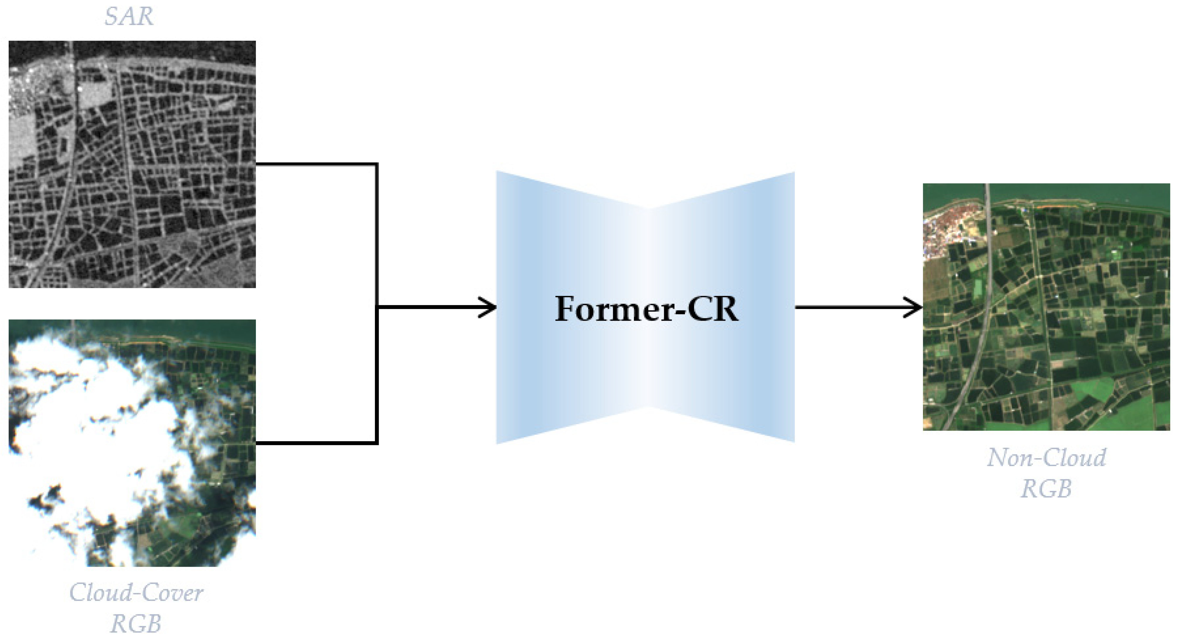
Figure 1. Flowchart of the proposed method.
Remotesensing 15 01196 g001
Figure 2. Former-CR network architecture.
Remotesensing 15 01196 g002
Figure 3. Lewin Transformer and down/up sample architecture.
Remotesensing 15 01196 g003
Figure 4. Decloud-IR network architecture.
Remotesensing 15 01196 g004
Figure 5. Results of Scene 1. (a) Input images, cloudy RGB and SAR images, from top to bottom. (b) SAR-Opt-cGAN; (c) DSen2-CR; (d) GLF-CR; (e) Former-CR (ours); (f) target RGB image. The first row of (bf) takes a full view of the predicted image, while the second row takes a detailed view of the red box area. The size of each image is 256 × 256 pixels.
Remotesensing 15 01196 g005
Figure 6. Results of Scene 2. (a) Input images, cloudy RGB and SAR images, from top to bottom. (b) SAR-Opt-cGAN; (c) DSen2-CR; (d) GLF-CR; (e) Former-CR (ours); (f) target RGB image. The first row of (bf) takes a full view of the predicted image, while the second row takes a detailed view of the red box area. The size of each image is 256 × 256 pixels.
Remotesensing 15 01196 g006
Figure 7. Results of Scene 3. (a) Input images, cloudy RGB and SAR images, from top to bottom. (b) SAR-Opt-cGAN; (c) DSen2-CR; (d) GLF-CR; (e) Former-CR (ours); (f) target RGB image. The first row of (bf) takes a full view of the predicted image, while the second row takes a detailed view of the red box area. The size of each image is 256 × 256 pixels.
Remotesensing 15 01196 g007
Figure 8. Results of Scene 4. (a) Input images, cloudy RGB and SAR images, from top to bottom. (b) SAR-Opt-cGAN; (c) DSen2-CR; (d) GLF-CR; (e) Former-CR (ours); (f) target RGB image. The first row of (bf) takes a full view of the predicted image, while the second row takes a detailed view of the red box area. The size of each image is 256 × 256 pixels.
Remotesensing 15 01196 g008
Figure 9. Performance of different loss functions in three scenarios. For each scene, (a) SAR image; (b) cloudy image; (c) cloud-free image; (d) L1 loss only; (e) ours. The green box shows the magnification of the corresponding region. The size of each image is 256 × 256 pixels.
Remotesensing 15 01196 g009
Figure 10. Various indicators of different models. The results with text annotations are the results of previous experiments.
Remotesensing 15 01196 g010
Figure 11. Performance of different combinations of parameters in scene 1. (a) Cloudy image; (b) cloud-free image; (c) Model-T; (d) Model-N; (e) Model-B; (f) Model-M; (g) Model-L. The size of each image is 256 × 256 pixels.
Remotesensing 15 01196 g011
Figure 12. Performance of different combinations of parameters in scene 2. (a) Cloudy image; (b) cloud-free image; (c) Model-T; (d) Model-N; (e) Model-B; (f) Model-M; (g) Model-L. The size of each image is 256 × 256 pixels.
Remotesensing 15 01196 g012
Table 1. SSIM, PSNR and MAE results of four models.
SAR-Opt-cGANDSen2-CRGLF-CROurs
SSIM0.76237   ±   0.0428 0.6856   ±   0.0323 0.8072 ± 0.0514 0.8082   ±   0.0532
PSNR24.26   ±   0.56 21.39   ±   0.22 27.95   ±   0.17 28.73   ±   0.14
MAE0.04650.07530.02840.0263
Bold numbers mean the best results.
Table 2. PSNR, SSIM and L1 indexes of different loss functions.
L1 LossOurs
PSNR22.1428.67
L10.03520.0283
SSIM0.57350.8103
Bold numbers mean the best results.
Table 3. The illumination for combination of parameters.
C N i
Model-T16{1, 1, 1, 1,1}
Model-N16{2, 2, 2, 2,4}
Model-B16{4, 4, 4, 4,4}
Model-M32{1, 2, 4, 8,4}
Model-L32{4, 4, 4, 4,4}
T means tiny, N means normal, B means big, M means massive, and L means large.
Disclaimer/Publisher’s Note: The statements, opinions and data contained in all publications are solely those of the individual author(s) and contributor(s) and not of MDPI and/or the editor(s). MDPI and/or the editor(s) disclaim responsibility for any injury to people or property resulting from any ideas, methods, instructions or products referred to in the content.