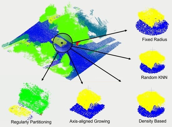
Article

Data Preparation Impact on Semantic Segmentation of 3D Mobile LiDAR Point Clouds Using Deep Neural Networks

by
Reza Mahmoudi Kouhi
1,*,
Sylvie Daniel
1 and
Philippe Giguère
2
1
Department of Geomatics Sciences, Université Laval, Québec City, QC G1V 0A6, Canada
2
Department of Computer Science and Software Engineering, Université Laval, Québec City, QC G1V 0A6, Canada
*
Author to whom correspondence should be addressed.
Remote Sens. 2023, 15(4), 982; https://doi.org/10.3390/rs15040982
Submission received: 28 November 2022 / Revised: 3 February 2023 / Accepted: 5 February 2023 / Published: 10 February 2023
(This article belongs to the Special Issue Semantic Segmentation Algorithms for 3D Point Clouds)

Abstract

:
Currently, 3D point clouds are being used widely due to their reliability in presenting 3D objects and accurately localizing them. However, raw point clouds are unstructured and do not contain semantic information about the objects. Recently, dedicated deep neural networks have been proposed for the semantic segmentation of 3D point clouds. The focus has been put on the architecture of the network, while the performance of some networks, such as Kernel Point Convolution (KPConv), shows that the way data are presented at the input of the network is also important. Few prior works have studied the impact of using data preparation on the performance of deep neural networks. Therefore, our goal was to address this issue. We propose two novel data preparation methods that are compatible with typical density variations in outdoor 3D LiDAR point clouds. We also investigated two already existing data preparation methods to show their impact on deep neural networks. We compared the four methods with a baseline method based on point cloud partitioning in PointNet++. We experimented with two deep neural networks: PointNet++ and KPConv. The results showed that using any of the proposed data preparation methods improved the performance of both networks by a tangible margin compared to the baseline. The two proposed novel data preparation methods achieved the best results among the investigated methods for both networks. We noticed that, for datasets containing many classes with widely varying sizes, the KNN-based data preparation offered superior performance compared to the Fixed Radius (FR) method. Moreover, this research allowed identifying guidelines to select meaningful downsampling and partitioning of large-scale outdoor 3D LiDAR point clouds at the input of deep neural networks.

Graphical Abstract

1. Introduction

A common representation for 3D objects and outdoor scenes is a 3D point cloud, which can be obtained by mobile terrestrial LiDAR. LiDAR point clouds record depth information, which, in contrast to images, can be used to accurately localize objects and characterize their shapes [1]. This makes them preferable in many applications such as building digital twin cities, urban management, and autonomous vehicles. However, besides georeferenced coordinates and intensity, raw point clouds have no information such as semantic information or object identification that could be straightforwardly used in downstream applications. Therefore, they have to be processed and labeled in order to provide such information [1,2,3]. Currently, image processing is dominated by the use of deep learning, in particular convolutional neural networks, which combine the local neighborhood features on 2D grids. This operation is made possible thanks to the grid structure of images. However, unlike images, 3D mobile LiDAR point clouds are unstructured. Therefore, dedicated approaches have been devised to use the point cloud at the input of the network [1]. Early solutions investigated different approaches to provide the point clouds with some structure: multi-view projection [4,5,6], voxelization [2,7,8], and octree-based structuring [9,10]. However, they were not adapted to large-scale point clouds or their point density heterogeneity, yielding inefficiency or the loss of valuable information [11,12,13]. Given such limits, solutions directly using the native point cloud have been designed. However, the size of these 3D point clouds prevents their use as a single input in deep neural networks. Indeed, outdoor scenes tend to be massive. For instance, SemanticKITTI contains more than four billion labeled points [14]. In order to avoid such a problem, the original point cloud is processed in subsets. In PointNet [11], the first network to use the native point cloud, semantic segmentation is performed by sampling the point cloud into 1 × 1 × 1 meter blocks. Then, points inside the blocks are processed individually. Other networks such as KPConv [15] use Random Sampling (RS) to select some spheres from the original point cloud as the input of the network. While current works focus generally on the architecture itself, few works have focused on the data preparation itself before the network and its impact on the network performance.
In the context of our paper, “Data preparation” means selecting a meaningful group of points from large-scale outdoor 3D LiDAR point clouds for the input of the neural networks. Although a few papers such as KPConv tried to tackle the problem of data preparation before the network, this is still an open research question. Therefore, this paper focuses only on this problem. To this end, we propose two novel data preparation methods along with investigating two already existing ones to illustrate the impact of using meaningful data samples at the input of deep neural networks. They are built toward the selection of meaningful groups of points for the input of deep neural networks. Generally, these methods consist of two parts, namely sampling and grouping, in order to generate the partitioning of the point sets. To assess the influence of the investigated methods on deep neural networks, we compared them with a baseline method that does not involve any data preparation and is based on point cloud regular partitioning in PointNet++. Regular partitioning is one of the simplest and most-straightforward techniques to select points at the input of the network. We used two deep neural networks, which are based on very different architectures: PointNet++ (point-based) [16] and KPConv (CNN-based) [15], to ensure that the performance variations are related to the data preparation and not the networks.
The key contributions of our work are as follows:
  • New insights into the impacts of the data preparation choices on deep neural networks. These insights were gained by comparing different grouping methods for different sequences of the dataset, analyzing the number of points per group in different layers of KPConv, the comparison of different sampling methods, and comparing the number of classes per group in different data preparation methods.
  • New general guidelines to intelligently select, that is adapted to the characteristics of the point clouds, a meaningful neighborhood and manage large-scale outdoor 3D LiDAR point clouds at the input of deep neural networks.
  • Two novel data preparation methods, namely Density Based (DB) and Axis Axis-Aligned Growing (AAG), which are compatible with outdoor 3D LiDAR point clouds and achieved the best results among the investigated data preparation methods for both KPConv and PointNet++.
The rest of the paper is organized as follows. A brief review of existing works related to deep neural networks and large-scale LiDAR point clouds is provided in Section 2. It underlines as well how data preparation is tackled in such networks. Then, the dataset and results are presented in Section 3. A thorough analysis and discussion of the results are presented in Section 4 before concluding.

2. Related Works

Here, we briefly review existing deep neural networks to process point clouds, paying special attention to methods involving data preparation either within the network or as a separate stage before the training. As underlined before, only networks processing native 3D point clouds are discussed. Qi et al. [11] are among the pioneer researchers who conducted such work. They introduced PointNet and PointNet++ [16]. PointNet [11] is among the first networks to consume unstructured and irregular point clouds. To do this, it divides the point cloud into blocks and then processes them individually. However, the results showing the network performances were sensitive to the size and number of points in the sampling blocks used by the network [17]. Therefore, PointNet++ [16] was introduced to overcome this limitation. Figure 1a shows its architecture. Unlike PointNet, PointNet++ is a hierarchical neural network. It applies PointNet as a feature learner on a partitioned point cloud recursively. In order to overcome the problems with PointNet++ and improve the performance of point-based networks, several other methods [12,18,19,20,21,22] have been proposed. For example, Engelmann et al. [12] proposed two mechanisms to add spatial context to PointNet in order to process large-scale point clouds: “multi-scale blocks” and “grid blocks”. In “multi-scale blocks”, a group of blocks at the same position, but at different scales is processed simultaneously, while, in “grid blocks”, a group of blocks is selected according to neighboring cells in a regular grid. Although the new architectures improve the performance of PointNet++ and overcome its problems (such as neglecting local features), most of them use the same method for preparing the data for processing, i.e., partitioning the point cloud into blocks. Moreover, another shortcoming of these methods is the fixed size of the point cloud subsets used at the input of the deep neural network. However, since the density of the point clouds is non-uniform, there are significantly more points within some subsets and not enough points in others [13]. Thus, issues of undersampling or data augmentation need to be addressed in such a context.
More recently, the kernel point fully convolutional network was introduced based on KPConv [15]. Figure 1b shows the architecture of this network. Unlike the previous deep learning methods for processing 3D native point clouds, KPConv includes an additional stage for data preparation before the training. In this stage, random spheres are selected from the original point cloud to form the input data of the network. These random spheres are created using radius-based neighborhoods instead of K-Nearest Neighbors (KNN) (which is used in similar networks, such as [23,24,25,26]) in order to keep a consistent receptive field. In addition to the random spheres, grid subsampling was added in each layer to increase the robustness of the network in the case of a highly uneven density of the input point cloud [27,28]. However, this addition causes the subsample clouds to contain a different number of points per cloud [15]. Therefore, the use of batches is not feasible, which leads to a longer training time. Although a solution consisting of concatenating batches has been proposed, the problem still exists when using massive large-scale point clouds, such as aggregated sequences of the SemanticKITTI dataset. Indeed, the network is unable to take the whole sequence in a single pass due to memory limitations [29].

3. Materials and Methods

In this section, we explain the methodology of the proposed data preparation methods, involving the following parameters: N the number of points in the original point cloud, S the number of seed points to generate groups for the input of the networks, K the number of nearest neighbors that determine the number of points in each group, B the size of the blocks used to partition the original point cloud (for time and memory efficiency), and R the radius of the sphere used to select points around seed points.

3.1. Random-KNN (R-KNN)

The first step in prepossessing large point clouds is to select groups from the original dataset. This can be accomplished by choosing seed points as the centroids of the groups. There are different methods to select these seed points. The most straightforward one consists of using RS, in which S seed points are uniformly selected from the original N points. It has high computational efficiency ( O ( 1 ) ), regardless of the scale of the input data [29].
Given N input points, S seed points are selected using RS:
S = ( N / K ) × 2 ,
where K is the number of nearest neighbors to each seed point that is selected using the KNN technique. On average, each point is assigned to at least two groups if the number of seed points (S) is calculated using Equation (1). The number of groups is the same as the number of seed points. This means that some groups have overlaps, which can lead to good coverage of the whole point cloud. Algorithm 1 describes the procedure of the R-KNN method.
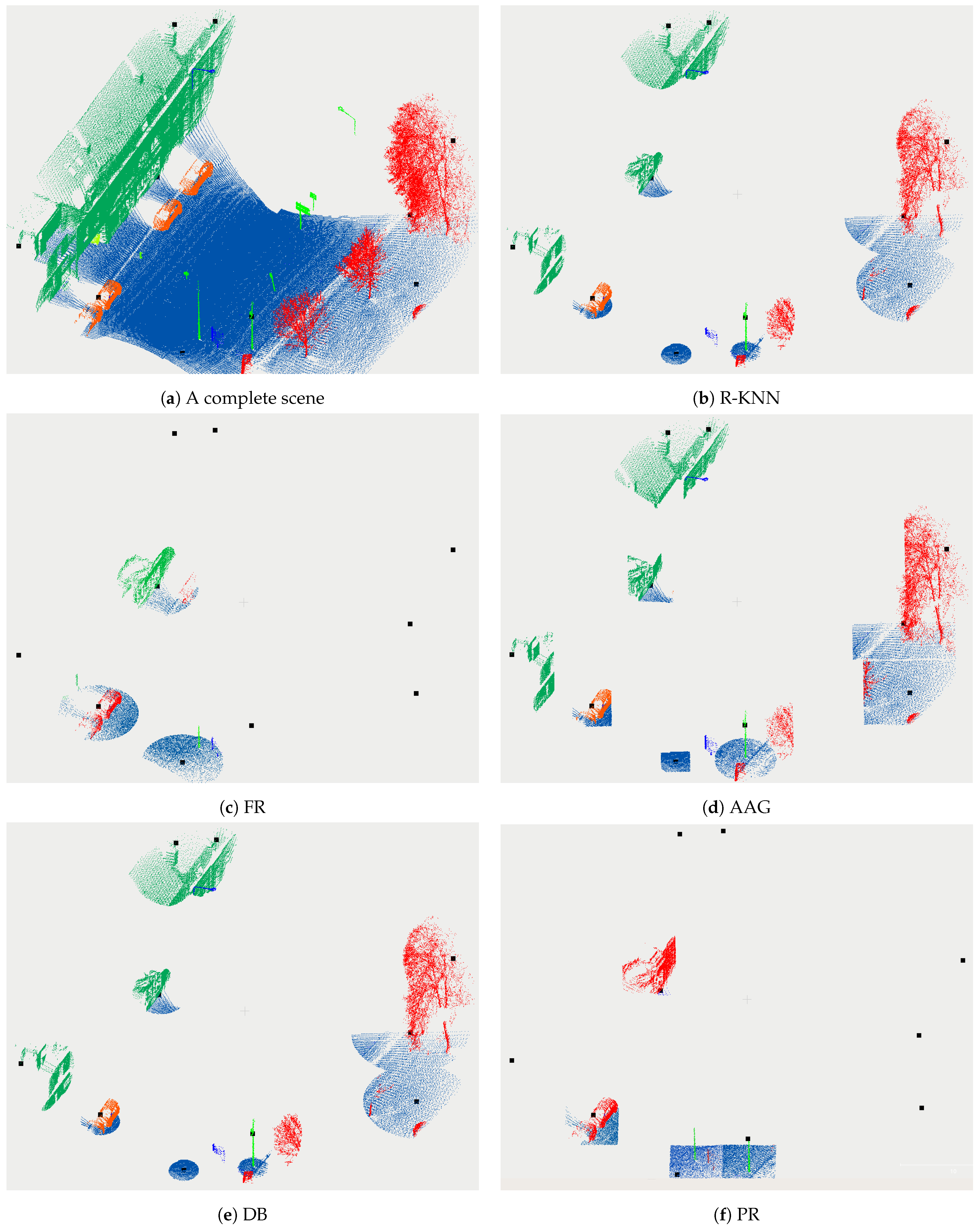
Figure 2 shows examples of using different grouping methods for the same seed points. Figure 2a displays the original point cloud of the scene. The generated groups using R-KNN are shown in Figure 2b.
Algorithm 1 R-KNN.
Require:
P , a l i s t o f p o i n t s
Require:
K , n u m b e r o f p o i n t s i n e a c h g r o u p o f p o i n t s
1:
S e e d _ P o i n t s S s e e d p o i n t s r a n d o m l y s e l e c t e d f r o m P
2:
for all  s S e e d _ P o i n t s   do
3:
     G r o u p _ P o i n t s s K - n e a r e s t n e i g h b o r s o f s i n P
4:
end for

3.2. Fixed Radius (FR)

In the FR data preparation, S seed points are selected randomly from the whole dataset, as in the R-KNN method. Then, instead of using KNN to create the groups, a fixed radius R around each seed point is used to select points to form the groups. If there are more than K points in the group, K points are randomly selected. Groups with less than K points are removed. The main difference between the fixed radius and KNN selection is as follows: the KNN spatial coverage shrinks in high-density areas and grows in sparse ones, while the fixed radius spatial coverage is constant regardless of the local point density. The shape of the selected groups using FR is displayed in Figure 2c. Algorithm 2 synthesizes the main steps of the FR method.
Algorithm 2 FR.
Require:
P , a l i s t o f p o i n t s
Require:
K , n u m b e r o f p o i n t s i n e a c h g r o u p o f p o i n t s
Require:
R , r a d i u s a r o u n d s e e d p o i n t s t o c r e a t e g r o u p s o f p o i n t s
1:
S e e d _ P o i n t s S s e e d p o i n t s r a n d o m l y s e l e c t e d f r o m P
2:
for all  s S e e d _ P o i n t s   do
3:
     G r o u p _ P o i n t s s P o i n t s i n a s p h e r e w i t h R r a d i u s f r o m s
4:
    if  L e n ( G r o u p _ P o i n t s s ) < K  then
5:
         D e l e t e G r o u p _ P o i n t s s
6:
    else
7:
         G r o u p _ P o i n t s s K p o i n t s r a n d o m l y s e l e c t e d f r o m G r o u p _ P o i n t s s
8:
    end if
9:
end for

3.3. Axis-Aligned Growing (AAG)

We devised Axis-Aligned Growing (AAG), described by Algorithm 3, as a new data preparation method. It picks S seed points randomly as in R-KNN and FR. The points belonging to the groups are selected through the growth of a bounding box around each seed until there are at least K points in the group. The growth is performed along the axes, for computational efficiency, and because the Z axis is aligned with the ground elevation. If there are more than K points in the group, K points are randomly selected. Thus, all the groups have an equal number of points for the input of the deep neural networks. Even if the seed points are selected randomly when using either R-KNN, FR, or AAG, the shape of their groups differs among these methods since their point selection approach is different. For AAG, the group shape is similar to a rectangular box (Figure 2d).

3.4. Density-Based (DB)

We devised Density-Based (DB) as a second novel data preparation method. Its principle consists of leveraging the uneven point density in the point cloud. A relatively dense group of points is generally associated with the presence of one or more objects. To compute the density map of the entire point cloud, we used the Kernel Density Estimation (KDE) function [30]. In statistics, KDE is a non-parametric method to estimate the probability density function of a random variable. Let ( p 1 , p 2 , , p n ) be a group of points with an unknown density f at any given point p. The kernel density estimator is:
f ^ h ( p ) = 1 n i = 1 n K h ( p p i ) = 1 n h i = 1 n K ( p p i h ) ,
where K is the kernel—a non-negative function—and h > 0 is a smoothing parameter called the bandwidth. A kernel with subscript h is called the scaled kernel and is defined as K h ( x ) = 1 / h K ( x / h ) .
Algorithm 3 AAG.
Require:
P , a l i s t o f p o i n t s
Require:
b 0 , i n i t i a l s i z e o f t h e b o x c o n t a i n i n g t h e g r o u p o f p o i n t s
Require:
K , n u m b e r o f p o i n t s i n e a c h g r o u p o f p o i n t s
1:
S e e d _ P o i n t s S s e e d p o i n t s r a n d o m l y s e l e c t e d f r o m P
2:
for all  s S e e d _ P o i n t s   do
3:
     s x , s y , s z S e e d _ P o i n t s [ s ]
4:
     b b 0
5:
    while  T r u e :  do
6:
         G r o u p _ P o i n t s s = [ ]             ▹ Create an empty list to store group points related to s
7:
        for all  p P  do
8:
            p x , p y , p z P [ p ]
9:
           if  a b s ( s x p x ) < b  then
10:
               if  a b s ( s y p y ) < b  then
11:
                   if  a b s ( s z p z ) < b  then
12:
                        G r o u p _ P o i n t s s . a p p e n d ( p )
13:
                   end if
14:
               end if
15:
           end if
16:
        end for
17:
         b b + 0.1
18:
        if  L e n ( G r o u p _ P o i n t s s ) > = K  then
19:
            G r o u p _ P o i n t s s K p o i n t s r a n d o m l y s e l e c t e d f r o m G r o u p _ P o i n t s s
20:
            B r e a k
21:
        end if
22:
    end while
23:
end for
After computing the density, points in the cloud are categorized into three classes according to the point density at their location: low, medium, and high. Then, seed selection is performed according to each density class separately. Since the point cloud consists mostly of points belonging to the medium-density class, a greater number of seed points need to be selected at such locations to ensure that the entire scene has been sampled. Selecting seed points separately, in locations with different point densities, provides a balanced selection of seed points all over the point cloud. Moreover, this approach allows taking into account objects that are located both near and far from the mobile LiDAR that recorded the point cloud. The selection of S seed points is performed by using the Farthest Point Sampling (FPS) method as specified by Algorithm 4. In a point cloud with N points, FPS selects S points, each of them being the farthest point from the first S 1 points.
Algorithm 4 FPS.
Require:
A l i s t o f p o i n t s ( P )
Require:
S , n u m b e r o f s e e d p o i n t s
1:
p 0 P i ,                                                         ▹i is selected randomly
2:
F a r t h e s t _ P o i n t s p 0
3:
d i s 0 A l i s t o f d i s t a n c e s o f e a c h p o i n t i n P f r o m p 0
4:
for  i 1 , S   do
5:
     d i s m a x _ i M a x i m u m o f d i s 0
6:
     i n d I n d e x o f t h e d i s m a x _ i i n P
7:
     F a r t h e s t _ P o i n t s [ i ] P [ i n d ]
8:
     d i s 1 D i s t a n c e s o f a l l p o i n t s i n P t o p 0
9:
     d i s 0 m i n ( d i s 0 , d i s 1 )
10:
end for
FPS was used in [16,24] for semantic segmentation of small-scale point clouds. Although it has good coverage of the entire point set, it has high computational complexity (( O N 2 )), especially for large-scale datasets [29]. The final step of the DB method consists of selecting the points to form the group. The KNN technique is used to this end. Algorithm 5 presents the procedure of the DB method. Figure 2e shows the shape of the groups provided by the DB method.
Algorithm 5 DB.
Require:
A l i s t o f p o i n t s ( P )
Require:
K , n u m b e r o f p o i n t s i n e a c h g r o u p
1:
D A l i s t o f d e n s i t y v a l u e s o f e a c h p o i n t i n P c a l c u l a t e d b y K D E
2:
L o w D & M e d D & H i g h D L i s t s o f P o i n t s i n l o w / m e d i u m / h i g h d e n s i t y z o n e s
3:
S h i g h & S l o w ( N / K ) / 2
4:
S m e d ( N / K )
5:
S e e d _ P o i n t s l o w F P S ( L o w D , S l o w )
6:
S e e d _ P o i n t s m e d F P S ( M e d D , S m e d )
7:
S e e d _ P o i n t s h i g h F P S ( H i g h D , S h i g h )
8:
for all  s S e e d _ P o i n t s   do
9:
     G r o u p _ P o i n t s s K - n e a r e s t n e i g h b o r s o f s i n P
10:
end for

3.5. Regularly Partitioning (RP)

Regularly Partitioning (RP) the point cloud is the data preparation method used in PointNet++. As a result, RP is considered as the baseline in this work. In PointNet++, the point cloud is partitioned into blocks of points. Each block should have K points. Therefore, if the partition creates blocks with less than K points, they are removed. For blocks with more than K points, a random selection of K points is conducted. Figure 2f shows the group shapes generated using this method.

4. Results

This section presents the performance results of the four data preparation methods discussed in Section 3. Beforehand, we present the implementation configuration and the dataset that was used in all the experiments, along with the procedure to split the dataset into the train, validation, and test sets.

4.1. Dataset and Implementation Configuration

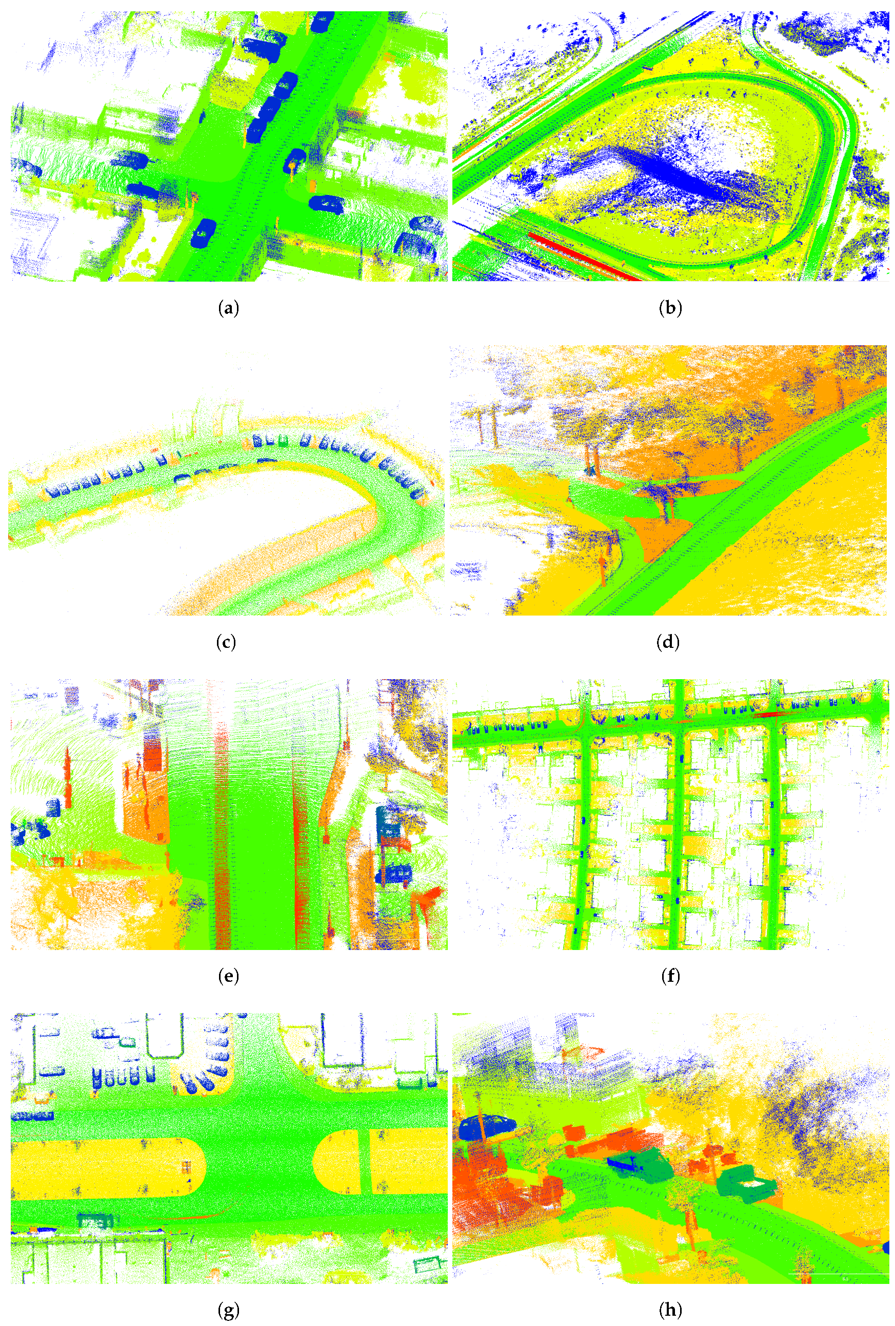
For benchmarking purposes, we evaluated the data preparation methods with the SemanticKITTI dataset [14]. SemanticKITTI should not be regarded as one dataset. In fact, it consists of 21 sequences (11 sequences with labeled points) consisting of 43,552 densely annotated LiDAR scans. Each scan covers approximately an area of 160 × 160 × 20 meters. The number of points per scan is about 10 5 . The focus of this work was massive large-scale outdoor 3D LiDAR point clouds, such as Paris-Lille-3D [31], which could be used in applications such as 3D HD maps for urban management purposes. This application context restricts the public datasets of interest. Indeed, S3DIS [32] involves only indoor scenes. Semantic3D [33] consists of static LiDAR acquisitions with limited outdoor spatial coverage. The ARCH dataset [34] focuses on historical built heritage. Since the SemanticKITTI dataset consists of sequential scans dedicated to autonomous vehicle applications, we performed a scan aggregation operation on each sequence of the SemanticKITTI dataset and used the aggregated point clouds to evaluate the data preparation methods. Figure 3 shows the diversity of this dataset, including intersections, parks, parking lots, cars with different sizes and parked or headed toward different directions, complex scenes with multiple objects, autoroutes, overpass bridges, and residential neighborhoods, to name a few. The SemanticKITTI scene semantic segmentation competition imposes Sequences 00∼07 and 09∼10 (19,130 scans) for training, Sequence 08 (4071 scans) for validation, and Sequences 11∼21 (20,351 scans) for online testing. However, since the objective of this paper was to illustrate the impact of data preparation on deep neural networks and not to compete with the state-of-the-art, we used the provided sequences differently. Instead, we performed a 10-fold cross-validation scheme for each data preparation method using Sequences 00∼07 and 09∼10.
Benchmarking was conducted to assess the impact of the proposed data preparation methods on the PointNet++ and KPConv networks. RP was used as a baseline. Relevant values were used for the main parameters involved in these methods. For consistency reasons, regarding the number of input points, K = 8192 was chosen as the number of points in each group, since this is the requested number of points at the input of PointNet++. In RP, to ensured we had 8192 points in the blocks, and we determined that the block size B should be 5 × 5 × 5 meters. We used a fixed radius (R) of 2 meters in the FR method. This value was selected as the average block size of the AAG method. In DB, KDE was calculated using the Gaussian KDE function of the Scipy library in python [35], which includes automatic bandwidth determination. The threshold values for determining low and high-density areas were set at 30% and 70% of the maximum density, respectively. The interval between 30 and 70% was considered as medium-density areas. We used 100 epochs to train the networks. In each epoch, 20,000 groups were randomly selected for training. The initial learning rate was set to 0.001 .

4.2. Semantic Segmentation Using the Data Preparation Methods

Table 1 and Table 2 present the mean Intersection over Union (mIoU) scores over 20 classes using PointNet++ and KPConv, respectively, and each one of the four data preparation methods. The performances of the data preparation methods were all better than the baseline by a significant margin. In PointNet++, using data preparation instead of regularly partitioning of the point cloud increased the mIoU average of all the sequences by 16.7%. In KPConv, which is one of the rare networks that uses data preparation before training, the lack of data preparation yielded a drop of the mIoU by 9%. The best mIoU score with PointNet++ was achieved using AAG, while the best mIoU score with KPConv was achieved using DB. It is worth mentioning these results cannot be compared with those of PointNet++ and KPConv on the SemanticKITTI dataset published in [14]. Indeed, as explained, we used aggregated scans of each SemanticKITTI sequence, while the published results with PointNet++ involved a single scan, and KPConv involved only five aggregated scans. The performance results are further analyzed and discussed in the next section.

5. Discussion

In KPConv, the authors claimed that using randomly selected spheres (such as FR) could result in a better mIoU than using KNN (such as R-KNN). However, our experiments showed that this hypothesis highly depends on the dataset and its context. Based on our experiments, using FR led to better results on the datasets where fewer points were located in low-density areas. In the other words, FR is more relevant when using datasets involving a few classes of large structures (e.g., roads, vegetation), for which the point density is high. On the other hand, KNN showed greater performance for datasets consisting of many classes related to objects with uneven sizes, yielding a larger number of points with low density. Table 3 shows the ratio of low-density points in each sequence of the dataset, the preferred grouping method for each sequence based on the number of points with low density, and the mIoU score related to each sequence using two data preparation methods, FR and R-KNN, for both networks. Based on Table 3, Sequences 1, 3, 4, 5, and 9 had fewer points with low density, and the best mIoU score for both networks was reached using the FR grouping method. On the contrary, Sequences 0, 2, 6, 7, and 10 had more points with low density, and the best mIoU score for both networks was reached using the KNN grouping method.
It can be inferred from Table 3 that the mIoU score related to S.1 using FR with both PointNet++ and KPConv was better than R-KNN with a margin of 2%. However, this was the opposite for S.2. This can be explained by analyzing the context of these two sequences. Analyzing the ratio of points in each sequence could help better understand the dependency of the FR and KNN performance on the context of the dataset. Table 4 shows the proportion of each class in the groups created, respectively, with R-KNN and FR and in the original dataset for the two sequences S.1 and S.2. As can be seen in this table, S.1 is an unbalanced dataset, for which the majority of the points belong to major classes such as road and vegetation. On the contrary, S.2 consists of points that belong not only to major classes, but also to classes related to smaller objects, such as cars, motorcycles, and buses. In S.1, for some classes with very few points such as building, the R-KNN method was able to generate groups of points from the original dataset, while FR failed. The reason is the nature of the FR method, which creates groups regardless of the local density. As shown in Figure 2c, some groups could not be created using the FR method because there were not enough points around the seed points with low density. Thus, using FR will result in neglecting objects with a low point density, ultimately affecting the balance of the training datasets and the resulting mIoU of the semantic segmentation. On the other hand, R-KNN always creates groups that contain the same number of points (K) irrespective of the local density. As can be seen in Figure 2b, R-KNN can create groups with both high and low-density.
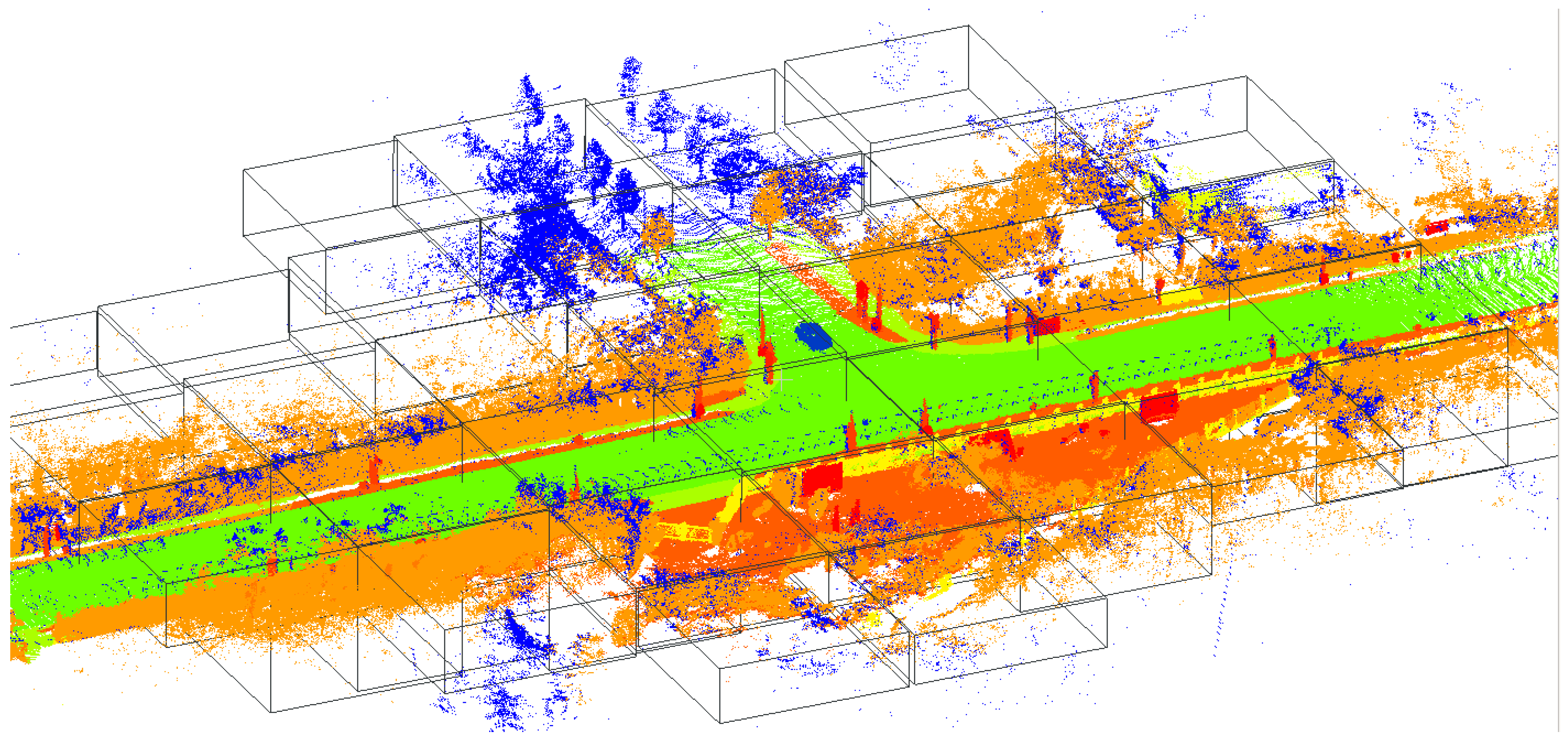
In [16,36], the authors claimed that using FPS will increase the mIoU score due to the good coverage of the selected seed points over the input point cloud. Figure 4 shows an example of such coverage using (a) RS and (b) FPS. As can be observed, FPS provides better coverage of the point cloud than RS; the latter naturally leads to a non-uniform sampling result, which focuses on points at locations with high density. However, when looking at Table 1 and Table 2, the mIoUs of R-KNN with RS are slightly lower than the mIoUs of DB using FPS. Therefore, when considering the significant processing time and memory usage of FPS, RS appears to be a relevant method to select seed points, especially with large-scale outdoor 3D LiDAR point clouds. To overcome the low efficiency of FPS, we propose a two-step solution for sampling large-scale outdoor 3D LiDAR point clouds. As shown in Figure 5, the first step consists of dividing the point cloud into blocks that are large enough that they can include the largest object in the scene. Then, the second step consists of downsampling each block to reduce the number of points. The downsampling is performed using a dropping point technique with a stride of 32. Applying this approach, FPS can be executed in a fair amount of time even with large-scale outdoor 3D LiDAR point clouds. In order to justify this statement, Table 5 shows the time (seconds) needed to select 100 seed points from three point clouds of size 10 5 , 10 6 , and 10 7 , respectively, using RS, FPS, and the improved FPS with downsampling. Using RS requires less than a second while, using FPS, 3178 s are needed to select the same number of seed points. However, using the improved FPS, this time is reduced to only 103 s. One could argue that this downsampling could affect the coverage of FPS over the complete point cloud. As is shown in Figure 4c, the coverage of seed points is the same if FPS or the improved FPS is used. For the proposed benchmark, it would have been possible to multiply the combinations of methods between those available for seed point selection and those for grouping. However, the possibilities are numerous, and the datasets used are also very large (i.e., four billion points), which makes the realization of such tests prohibitive. The objective of this research was not to test all possible cases, but to highlight the impact of the chosen methods on the performance of the network. In addition, the proposed benchmark is sufficiently comprehensive to propose general guidelines one may use to find a suitable combination of seed selection and grouping methods for one dataset.
Figure 2e shows that groups created with DB have almost the same shape as the R-KNN groups (Figure 2b). This was expected because both of their grouping methods are based on KNN. However, the higher mIoU score achieved by DB in both PointNet++ and KPConv makes DB a better data preparation method in comparison to R-KNN. This underlines the advantage of KDE and FPS to create groups.
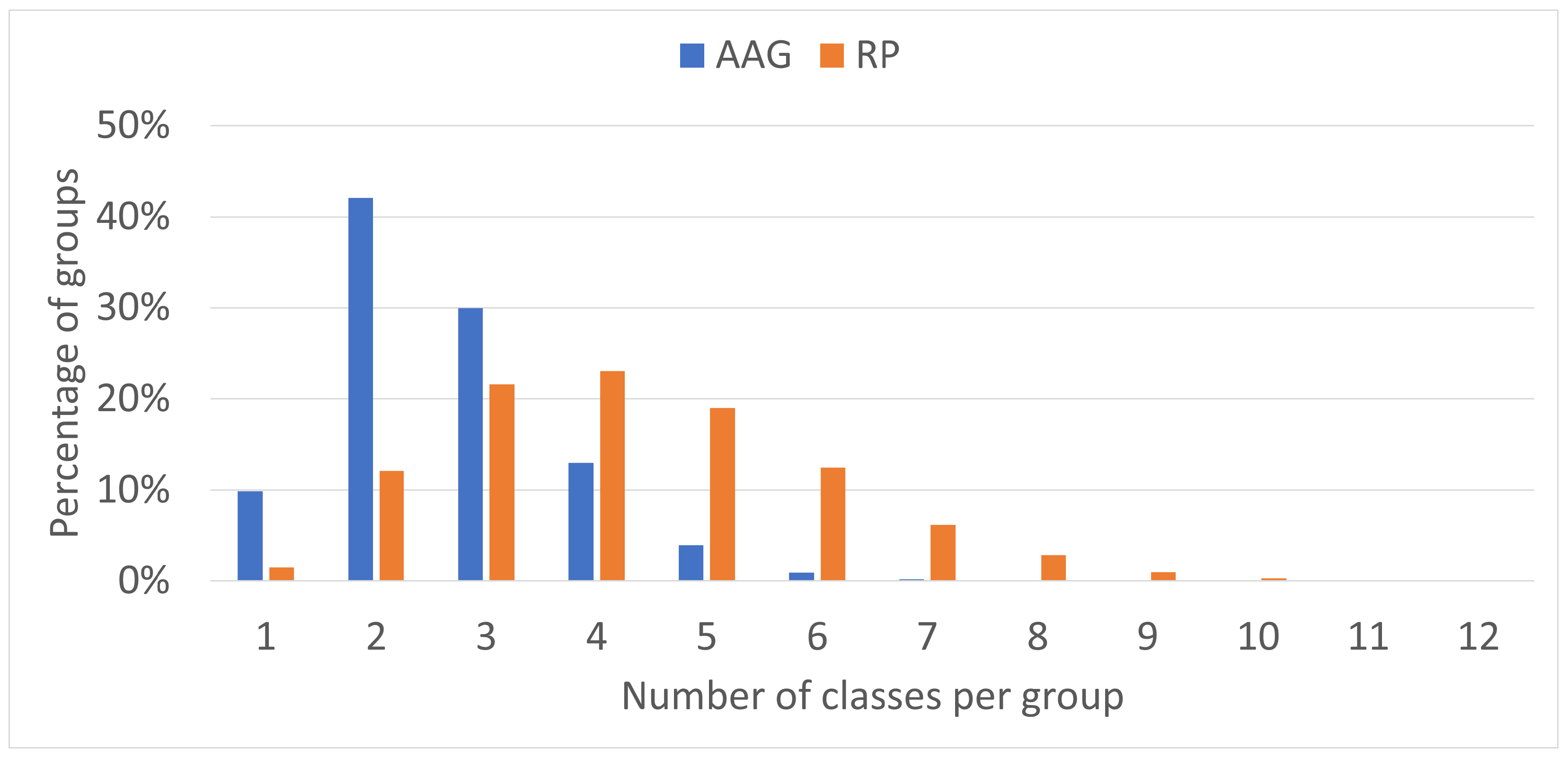
The shapes of AAG groups are quite similar to those of RP groups since both of them are created using boxes, the former by growing a box around a seed point and the latter by partitioning the point cloud into boxes. However, using AAG, the mIoU score is more than twice better for PointNet++ and about 9% better for KPConv. This reveals two critical advantages of AAG over RP. First, randomly selecting seed points to create groups appears to be a better strategy than regularly partitioning the point cloud. Second, involving homogeneous, compact boxes is more informative than larger, heterogeneous boxes. Figure 6 shows the comparison of the number of classes per group for the two methods. The average number of classes in the AAG boxes is 2.6 , while the RP boxes contain 4.3 classes on average. Therefore, AAG creates more homogeneous, compact boxes than RP.
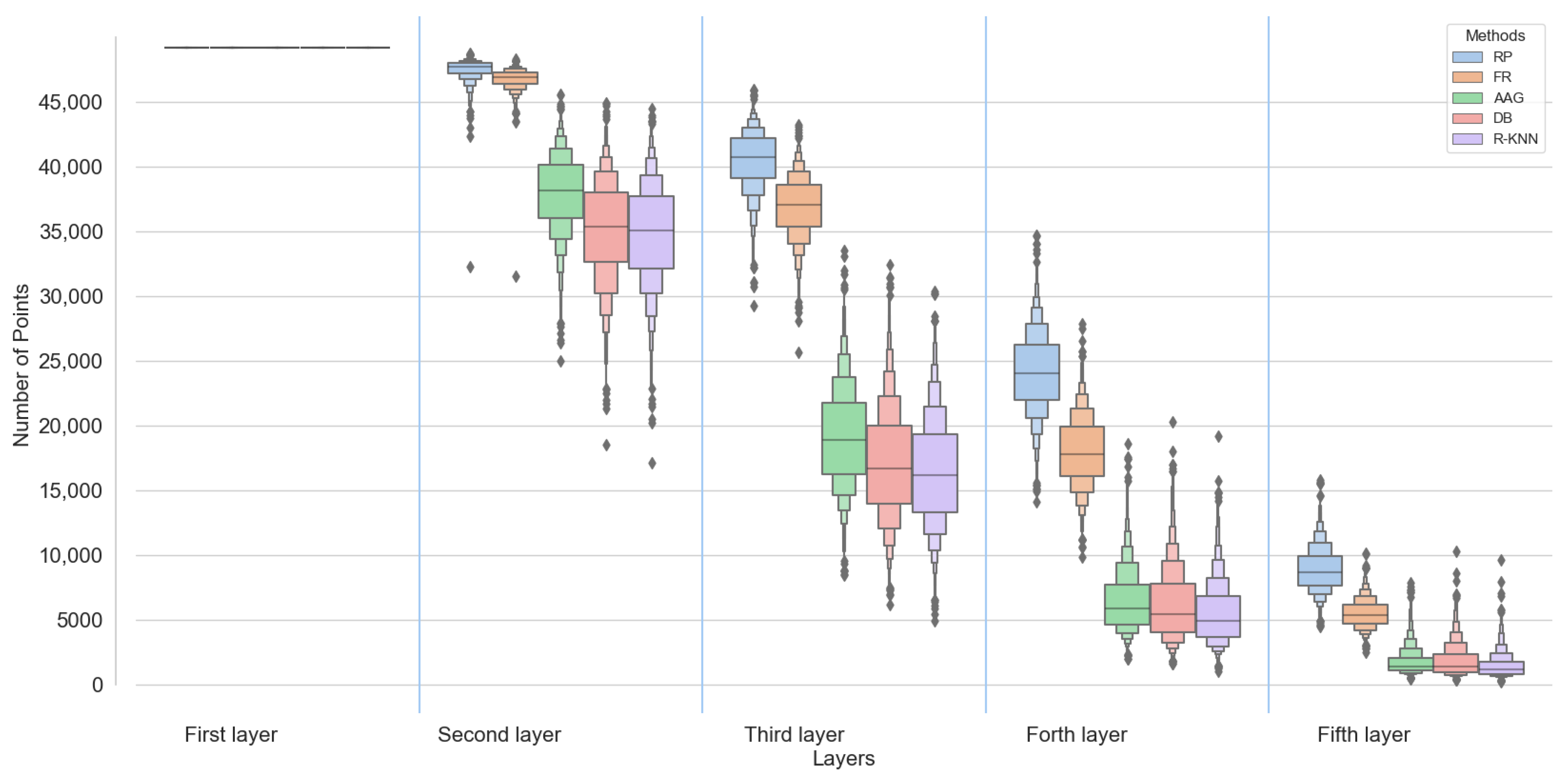
Table 6 shows the training time for one epoch, using an NVIDIA Quadro RTX 8000, for PointNet++ and KPConv using the data preparation methods and the number of groups created by each data preparation method. The number of groups is the same as the number of seed points. Using each one of these methods increased the number of groups significantly compared to RP and the original dataset. As shown in Equation (1), each point is assigned to at least two nearby seed points. Therefore, the proposed data preparation methods can be also regarded as data augmentation, which can improve the network’s performances and lead to a higher mIoU score. For PointNet++, the training time of all the data preparation methods was higher than the baseline. This was expected given the higher number of groups of all the methods compared to RP. The training time for PointNet++ was much lower than KPConv in all of the benchmarking. This was also expected given that the architecture of KPConv prevents the network from taking advantage of parallel batch processing. For KPConv, the training time using RP and FR was higher than the other methods. This was due to the number of points in each layer of KPConv when using different data preparation methods (Figure 7). KPConv has five layers, and each layer downsamples the input data to create the input of the next layer. The downsampling technique is based on the distribution of the points in the input point cloud. According to the KPConv downsampling technique, first, the input point cloud is divided into 3D grids and, then, the barycenter of each grid is used to create the input of the next layer [15]. The RP and FR groups are fixed-size neighborhoods. Points in these groups are spread and cause the next layer to have more points after the downsampling. In other words, the groups of these two methods cover more area than other methods while containing the same amount of points. A comparison of the training time of the FR method to the methods with the KNN-based grouping technique revealed another advantage of KNN for datasets containing more points with low density. Using FR for these datasets will create groups with a scattered distribution, which leads to a higher training time for architectures such as KPConv.
An improved version of FPS is proposed that could process large-scale outdoor 3D LiDAR point clouds in a fair amount of time. The improved FPS could sample the space better than RS and improve the performance of the networks.

6. Conclusions

In this work, we compared four different data preparation methods to select subsets of large-scale outdoor 3D LiDAR point clouds for deep neural networks. Selecting a group of points for the input of deep neural networks is a key step, and its importance should not be neglected. The basic idea of all the proposed methods is the same: first, selecting seed points and, then, grouping neighboring points around each seed point. The difference is in their methods to select the seed points or group neighboring points. We tested these methods on two popular deep neural networks, namely PointNet++ and KPConv. To assess their impact, we compared them to a baseline method, which regularly partitions the point clouds. Using any of the data preparation methods improved the performance of both networks by a tangible margin. For instance, the mIoU in PointNet++ and KPConv increased by 16.7% and 9%, respectively, in comparison to the baseline method.
The two proposed novel data preparation methods, namely DB and AAG, are compatible with typical density variations in large-scale outdoor 3D LiDAR point clouds and achieved the best results among the investigated data preparation methods for both KPConv and PointNet++. However, they are computationally more expensive than the other investigated methods. Among the grouping techniques, KNN showed superior performance compared to FR, where the datasets contain many classes with widely varying sizes. In addition, FPS has better coverage than RS, but it is time-consuming, especially for large-scale outdoor 3D LiDAR point clouds. Therefore, an improved version of FPS is proposed that could process large-scale outdoor 3D LiDAR point clouds in a fair amount of time. The improved FPS could sample the space better than RS and improve the performance of the networks.
Even if a comprehensive benchmark was proposed in this paper, we could not investigate all the possible combinations of the grouping and sampling methods due to time constraints. Thus, some combinations would be worth evaluating such as FPS seed point selection and AAG grouping, given the performance that each provided. It would then be interesting to determine the contexts favorable to such a combination. Furthermore, since our improved FPS is relatively simple, it would be appropriate to evaluate other approaches to reduce the prohibitive computational time of this method, or even an approach that would be a compromise between RS and FPS in terms of selected seed points and computational time. The research proposed in this paper has advanced the knowledge on the selection of regions of interest in the point cloud and subgroups of points in order to constitute the training samples of the network for an efficient segmentation, according to the inherent characteristics of the large-scale outdoor 3D point clouds. A new study could therefore take advantage of this knowledge to propose efficient sample selection solutions for networks for which the massive volume of these point clouds is an important issue (e.g., MinkowskiNet [37] and 3D Transformers [38]).

Author Contributions

Conceptualization, R.M.K., S.D., and P.G.; methodology, R.M.K., S.D. and P.G.; software, R.M.K.; validation, R.M.K., S.D. and P.G.; formal analysis, R.M.K., S.D. and P.G.; investigation, R.M.K.; resources, R.M.K., S.D. and P.G.; data curation, R.M.K.; writing—original draft preparation, R.M.K.; writing—review and editing, R.M.K., S.D. and P.G.; visualization, R.M.K.; supervision, S.D. and P.G.; project administration, S.D.; funding acquisition, S.D.; All authors have read and agreed to the published version of the manuscript.

Funding

This research was funded by the Natural Sciences and Engineering Research Council (NSERC) of Canada Grant Number RGPIN-2018-04046.

Data Availability Statement

The SemanticKITTI dataset’s official website is https://http://www.semantic-kitti.org/ (accessed on 25 November 2022).

Acknowledgments

The authors gratefully acknowledge the support of the NSERC grant, the Research Center in Geospatial Data and Intelligence of Université Laval, the Institute on intelligence and Data of Université Laval, NVIDIA for providing a high-performance GPU for our research project through their hardware acceleration program, and Compute Canada for providing us the opportunity to run our benchmarkings on their clusters.

Conflicts of Interest

The authors declare no conflict of interest.

Abbreviations

The following abbreviations are used in this manuscript:
Kernel Point Convolution (KPConv)
Fixed Radius (FR)
Random Sampling (RS)
K-Nearest Neighbors (KNN)
Density-Based (DB)
Axis-Aligned Growing (AAG)
Random-KNN (R-KNN)
Regularly Partitioning (RP)
Kernel Density Estimation (KDE)
Farthest Point Sampling (FPS)
mean Intersection over Union (mIoU)

References

  1. Otepka, J.; Ghuffar, S.; Waldhauser, C.; Hochreiter, R.; Pfeifer, N. Georeferenced Point Clouds: A Survey of Features and Point Cloud Management. ISPRS Int. J. -Geo-Inf. 2013, 2, 1038–1065. [Google Scholar] [CrossRef]
  2. Zhou, Y.; Tuzel, O. VoxelNet: End-to-end learning for point cloud based 3d object detection. In Proceedings of the IEEE Conference on Computer Vision and Pattern Recognition, Salt Lake City, UT, USA, 18–22 June 2018; pp. 4490–4499. [Google Scholar]
  3. Yousefhussien, M.; Kelbe, D.J.; Ientilucci, E.J.; Salvaggio, C. A multi-scale fully convolutional network for semantic labeling of 3D point clouds. ISPRS J. Photogramm. Remote. Sens. 2018, 143, 191–204. [Google Scholar] [CrossRef]
  4. Yu, T.; Meng, J.; Yuan, J. Multi-view Harmonized Bilinear Network for 3D Object Recognition. In Proceedings of the IEEE Conference on Computer Vision and Pattern Recognition, Salt Lake City, UT, USA, 18–22 June 2018. [Google Scholar]
  5. Yang, Z.; Wang, L. Learning Relationships for Multi-View 3D Object Recognition. In Proceedings of the IEEE International Conference on Computer Vision (ICCV), Seoul, Korea, 27 October–2 November 2019. [Google Scholar]
  6. Boulch, A.; Guerry, J.; Le Saux, B.; Audebert, N. SnapNet: 3D point cloud semantic labeling with 2D deep segmentation networks. Comput. Graph. 2018, 71, 189–198. [Google Scholar] [CrossRef]
  7. Hackel, T.; Savinov, N.; Ladicky, L.; Wegner, J.D.; Schindler, K.; Pollefeys, M. SEMANTIC3D.NET: A new large-scale point cloud classification benchmark. In ISPRS Annals of the Photogrammetry, Remote Sensing and Spatial Information Sciences; Copernicus GmbH: Göttingen, Germany, 2017. [Google Scholar]
  8. Huang, J.; You, S. Point cloud labeling using 3d convolutional neural network. In Proceedings of the IEEE International Conference on Pattern Recognition (ICPR), Cancun, Mexico, 4–8 December 2016; pp. 2670–2675. [Google Scholar]
  9. Riegler, G.; Ulusoy, A.O.; Geiger, A. OctNet: Learning Deep 3D Representations at High Resolutions. In Proceedings of the IEEE Conference on Computer Vision and Pattern Recognition, Honolulu, HI, USA, 21 July–26 July 2017. [Google Scholar]
  10. Wang, P.S.; Liu, Y.; Guo, Y.X.; Sun, C.Y.; Tong, X. O-CNN: Octree-based Convolutional Neural Networks for 3D Shape Analysis. ACM Trans. Graph. 2017, 36, 1–11. [Google Scholar] [CrossRef]
  11. Qi, C.R.; Su, H.; Mo, K.; Guibas, L.J. PointNet: Deep learning on point sets for 3d classification and segmentation. In Proceedings of the IEEE Conference on Computer VISION and Pattern recognition, Honolulu, HI, USA, 21 July–26 July 2017; pp. 652–660. [Google Scholar]
  12. Engelmann, F.; Kontogianni, T.; Hermans, A.; Leibe, B. Exploring Spatial Context for 3D Semantic Segmentation of Point Clouds. In Proceedings of the IEEE International Conference on Computer Vision Workshops (ICCVW), Venice, Italy, 22–29 October 2017. [Google Scholar]
  13. Griffiths, D.; Boehm, J. A Review on Deep Learning Techniques for 3D Sensed Data Classification. Remote. Sens. 2019, 11, 1499. [Google Scholar] [CrossRef]
  14. Behley, J.; Garbade, M.; Milioto, A.; Quenzel, J.; Behnke, S.; Stachniss, C.; Gall, J. SemanticKITTI: A Dataset for Semantic Scene Understanding of LiDAR Sequences. In Proceedings of the IEEE International Conference on Computer Vision (ICCV), Seoul, Korea, 27 October–2 November 2019. [Google Scholar]
  15. Thomas, H.; Qi, C.R.; Deschaud, J.E.; Marcotegui, B.; Goulette, F.; Guibas, L.J. KPConv: Flexible and Deformable Convolution for Point Clouds. In Proceedings of the IEEE International Conference on Computer Vision, Seoul, Korea, 27 October–2 November 2019. [Google Scholar]
  16. Qi, C.R.; Yi, L.; Su, H.; Guibas, L.J. PointNet++: Deep Hierarchical Feature Learning on Point Sets in a Metric Space. In Proceedings of the Advances in Neural Information Processing Systems 30: Annual Conference on Neural Information Processing Systems 2017, Long Beach, CA, USA, 4–9 December 2017; pp. 5099–5108. [Google Scholar]
  17. Guo, Y.; Wang, H.; Hu, Q.; Liu, H.; Liu, L.; Bennamoun, M. Deep Learning for 3D Point Clouds: A Survey. IEEE Trans. Pattern Anal. Mach. Intell. 2020, 43, 4338–4364. [Google Scholar] [CrossRef] [PubMed]
  18. Wang, Y.; Sun, Y.; Liu, Z.; Sarma, S.E.; Bronstein, M.M.; Solomon, J.M. Dynamic Graph CNN for Learning on Point Clouds. ACM Trans. Graph. (TOG) 2019, 38, 1–12. [Google Scholar] [CrossRef]
  19. Komarichev, A.; Zhong, Z.; Hua, J. A-CNN: Annularly Convolutional Neural Networks on Point Clouds. In Proceedings of the IEEE Conference on Computer Vision and Pattern Recognition, Long Beach, CA, USA, 15–20 June 2019. [Google Scholar]
  20. Su, H.; Jampani, V.; Sun, D.; Maji, S.; Kalogerakis, E.; Yang, M.H.; Kautz, J. SPLATNet: Sparse Lattice Networks for Point Cloud Processing. In Proceedings of the IEEE Conference on Computer Vision and Pattern Recognition, Salt Lake City, UT, USA, 18–22 June 2018. [Google Scholar]
  21. Wang, L.; Huang, Y.; Hou, Y.; Zhang, S.; Shan, J. Graph Attention Convolution for Point Cloud Semantic Segmentation. In Proceedings of the IEEE Conference on Computer Vision and Pattern Recognition (CVPR), Long Beach, CA, USA, 15–20 June 2019. [Google Scholar]
  22. Engelmann, F.; Kontogianni, T.; Schult, J.; Leibe, B. Know What Your Neighbors Do: 3D Semantic Segmentation of Point Clouds. In Proceedings of the IEEE European Conference on Computer Vision—ECCV Workshops, Long Beach, CA, USA, 16–21 June 2019. [Google Scholar]
  23. Xu, Y.; Fan, T.; Xu, M.; Zeng, L.; Qiao, Y. SpiderCNN: Deep Learning on Point Sets with Parameterized Convolutional Filters. In Proceedings of the IEEE European Conference on Computer Vision, Salt Lake City, UT, USA, 18–22 June 2018. [Google Scholar]
  24. Li, Y.; Bu, R.; Sun, M.; Wu, W.; Di, X.; Chen, B. PointCNN: Convolution On X-Transformed Points. In Proceedings of the Neural Inf. Process. Syst. (NIPS). arXiv 2018, arXiv:1801.07791. [Google Scholar]
  25. Groh, F.; Wieschollek, P.; Lensch, H.P.A. Flex-Convolution (Million-Scale Point-Cloud Learning Beyond Grid-Worlds). In Proceedings of the IEEE Asian Conference on Computer Vision (ACCV), Perth, Australia, 2–6 December 2018. [Google Scholar]
  26. Wang, S.; Suo, S.; Ma, W.C.; Pokrovsky, A.; Urtasun, R. Deep Parametric Continuous Convolutional Neural Networks. In Proceedings of the IEEE Conference on Computer Vision and Pattern Recognition, Salt Lake City, UT, USA, 18–22 June 2018. [Google Scholar]
  27. Thomas, H.; Deschaud, J.E.; Marcotegui, B.; Goulette, F.; Gall, Y.L. Semantic Classification of 3D Point Clouds with Multiscale Spherical Neighborhoods. In Proceedings of the IEEE International Conference on 3D Vision, Verona, Italy, 5–8 September 2018. [Google Scholar]
  28. Hermosilla, P.; Ritschel, T.; Vázquez, P.P.; Vinacua, À.; Ropinski, T. Monte Carlo convolution for learning on non-uniformly sampled point clouds. ACM Trans. Graph. 2019, 37, 1–12. [Google Scholar] [CrossRef]
  29. Hu, Q.; Yang, B.; Xie, L.; Rosa, S.; Guo, Y.; Wang, Z.; Trigoni, N.; Markham, A. RandLA-Net: Efficient Semantic Segmentation of Large-Scale Point Clouds. In Proceedings of the IEEE Conference on Computer Vision and Pattern Recognition, Seattle, WA, USA, 13–19 June 2020. [Google Scholar]
  30. Scott, D.W. Multivariate Density Estimation: Theory, Practice, and Visualization; John Wiley & Sons: Hoboken, NJ, USA, 2015. [Google Scholar]
  31. Roynard, X.; Deschaud, J.E.; Goulette, F. Paris-Lille-3D: A large and high-quality ground truth urban point cloud dataset for automatic segmentation and classification. Int. J. Robot. Res. 2018, 37, 545–557. [Google Scholar] [CrossRef]
  32. Armeni, I.; Sener, O.; Zamir, A.; Jiang, H.; Brilakis, I.; Fischer, M.; Savarese, S. 3D semantic parsing of large-scale indoor spaces. In Proceedings of the IEEE Conference on Computer Vision and Pattern Recognition, Las Vegas, NV, USA, 27–30 June 2016. [Google Scholar]
  33. Hackel, T.; Savinov, N.; Ladicky, L.; Wegner, J.; Schindler, K.; Pollefeys, M. SEMANTIC3D.NET: A new large-scale point cloud classification benchmark. arXiv 2017, arXiv:1704.03847. [Google Scholar] [CrossRef] [Green Version]
  34. Matrone, F.; Lingua, A.; Pierdicca, R.; Malinverni, E.S.; Paolanti, M.; Grilli, E.; Remondino, F.; Murtiyoso, A.; Landes, T. A Benchmark For Large-Scale Heritage Point Cloud Semantic Segmentation. Int. Arch.Photogramm. Remote Sens. Spat. Inf. Sci. 2020, 43, 1419–1426. [Google Scholar] [CrossRef]
  35. Virtanen, P.; Gommers, R.; Oliphant, T.E.; Haberland, M.; Reddy, T.; Cournapeau, D.; Burovski, E.; Peterson, P.; Weckesser, W.; Bright, J.; et al. SciPy 1.0: Fundamental Algorithms for Scientific Computing in Python. Nat. Methods 2020, 17, 261–272. [Google Scholar] [CrossRef] [PubMed] [Green Version]
  36. Boulch, A.; Puy, G.; Marlet, R. FKAConv: Feature-Kernel Alignment for Point Cloud Convolution. In Proceedings of the IEEE Asian Conference on Computer Vision, Kyoto, Japan, 30 November–4 December 2020. [Google Scholar]
  37. Choy, C.; JunYoung Gwak, S.S. 4D Spatio-Temporal ConvNets: Minkowski Convolutional Neural Networks. In Proceedings of the IEEE Conference on Computer Vision and Pattern Recognition (CVPR), Long Beach, CA, USA, 15–20 June 2019. [Google Scholar]
  38. Zhao, H.; Jiang, L.; Jia, J.; Tor, P.; Koltu, V. Point Transformer. In Proceedings of the IEEE International Conference on Computer Vision (ICCV), Montreal, BC, Canada, 11–17 October 2021. [Google Scholar]
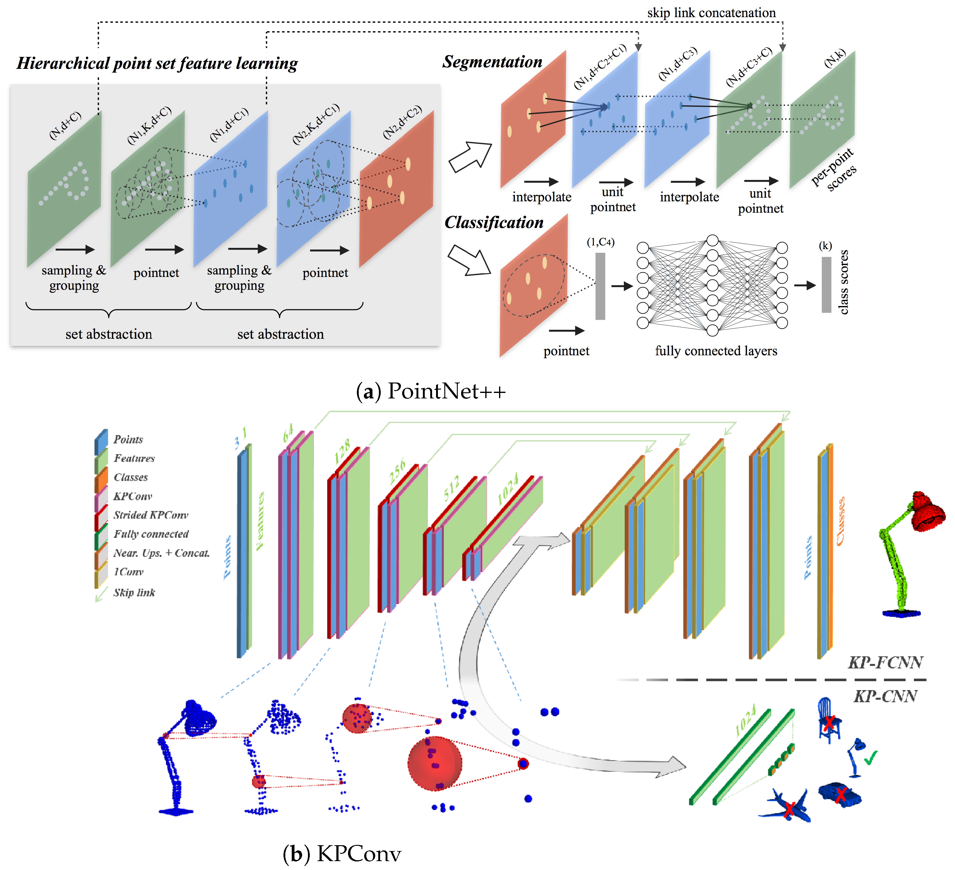
Figure 1. Architectures of PointNet++ (a) and KPConv (b) networks [15,16]. The encoder of both networks has a sampling and grouping stage, which makes the input point cloud ready for the network. However, both of these stages are inside the networks and cannot handle massive large-scale point clouds as the input due to memory limitations.
Remotesensing 15 00982 g001
Figure 2. Comparison of the impact of the grouping methods, illustrated using the same seed points. A complete scene (a) and groups of points with diverse shapes according to the selected data preparation methods, namely: R-KNN (b), FR (c), AAG (d), DB (e), and RP (f). The black dots represent the same seed points for all of the methods.
Remotesensing 15 00982 g002
Figure 3. Examples of urban scene diversity recorded in the SemanticKITTI dataset. (a) A complex scene of an intersection; (b) overpass bridge and autoroute mixed with vegetation; (c) a curvy street with cars parked in different directions; (d) a park; (e) parking lots and streets with a tram; (f) residential neighborhood; (g) a boulevard intersection with cars parked in different directions; (h) a complex urban scene including cars and trucks.
Remotesensing 15 00982 g003
Figure 4. Comparison of FPS and improved FPS (a) and sampled seed points using RS (b) for Sequence 4.
Remotesensing 15 00982 g004
Figure 5. Sequence 4 divided into blocks of 20 × 20 × 20 m to reduce FPS processing time.
Remotesensing 15 00982 g005
Figure 6. Histograms of the number of classes per group generated by RP and AAG data preparation methods.
Remotesensing 15 00982 g006
Figure 7. Number of points per layer of KPConv for the proposed data preparation methods.
Remotesensing 15 00982 g007
Table 1. Test results (mIoU %) of PointNet++ using different data preparation methods. S.X is the sequence number used as a test dataset. The mean (%) and standard deviation (%) of all the sequences’ mIoUs are provided for each data preparation method.
MethodsSeed
Selection
GroupingS.0S.1S.2S.3S.4S.5S.6S.7S.9S.10MeanStd
RP (baseline)Not usedNot used22.123.015.124.720.823.617.623.823.622.121.63.04
R-KNNRSKNN45.722.129.540.026.542.531.545.642.036.536.28.36
FRRSFixed radius45.225.726.444.930.744.631.043.642.536.037.18.02
AAG (ours)RSGrowing box47.725.231.742.826.448.234.045.942.439.038.38.54
DB (ours)FPSKNN46.628.628.938.732.743.931.244.140.036.737.16.59
Table 2. Test results (mIoU %) of KPConv using different data preparation methods. S.X is the sequence number used as a test dataset. The mean (%) and standard deviation (%) of all the sequences’ mIoUs are provided for each data preparation method.
MethodsSeed
Selection
GroupingS.0S.1S.2S.3S.4S.5S.6S.7S.9S.10MeanStd
RP (baseline)Not usedNot used40.221.227.136.330.438.530.539.438.335.433.86.24
R-KNNRSKNN48.029.535.043.837.144.640.847.343.242.541.25.78
FRRSFixed radius47.231.330.544.538.748.136.245.144.238.040.46.38
AAG (ours)RSGrowing box48.929.834.345.837.246.841.448.944.544.842.26.48
DB (ours)FPSKNN50.532.036.044.238.146.842.748.345.044.742.85.77
Table 3. Comparison of KNN and FR grouping methods’ performances for different sequences of the SemanticKITTI dataset.
SequencesmIoU FR
PointNet++ (%)
mIoU R-KNN
PointNet++ (%)
mIoU FR
KPConv (%)
mIoU R-KNN
KPConv (%)
Grouping Methods
Providing the Best mIoU
Ratio of Low-Density
Points (%)
S. 045.245.747.248.0KNN38
S. 125.722.131.329.5FR31
S. 226.429.530.535.0KNN42
S. 344.940.044.543.8FR32
S. 430.726.538.737.1FR33
S. 544.642.548.144.6FR31
S. 631.031.536.240.8KNN38
S. 743.645.645.147.3KNN42
S. 942.542.044.243.2FR33
S. 1036.036.538.042.5KNN38
Table 4. Class proportion (percentage) of the groups created with R-KNN and FR methods and in the original dataset for Sequences S.1 and S.2. S.2 has 17 classes, while S.1 has 11 classes (i.e., S.2 is more balanced than S.1). The absence of minor classes in S.1 means such classes will not be learned by the network.
ClassesS.1S.2
R-KNNFROriginalR-KNNFROriginal
Unlabeled3.081.113.651.481.401.89
Car0.000.000.742.322.082.23
Bicycle0.000.000.000.0030.0020.002
Motorcycle0.000.000.000.010.010.01
Other Vehicles0.000.000.060.050.030.05
Person0.000.000.000.0030.0040.01
Road40.1745.9540.5119.5119.3019.66
Parking0.000.000.002.172.272.19
Sidewalk0.00040.00050.000317.5918.5018.35
Other Ground3.063.302.630.090.120.12
Building0.220.000.205.815.625.87
Fence15.3015.6414.359.089.628.58
Vegetation23.5621.1223.5735.2834.9034.38
Trunk0.050.010.040.880.720.81
Terrain14.1812.5713.835.515.215.62
Pole0.200.190.220.180.190.20
Traffic Sign0.190.110.200.020.010.02
Table 5. Comparison of the time (seconds) needed to sample 100 points from three point clouds of size 10 5 , 10 6 , and 10 7 , respectively, using the following sampling methods: RS, FPS, and improved FPS with downsampling (DS).
Sampling Methods 10 5 10 6 10 7
RS0.00160.0130.24
FPS29.85298.373178.76
FPS + DS (ours)0.979.19103.47
Table 6. Training time for PointNet++ and KPConv using the proposed data preparation methods for one epoch and the number of groups created by the proposed data preparation methods.
MethodsPointNet++KPConvNumber of Groups
RP (baseline)4 min30 min30,020
R-KNN6 min21 min651,620
FR6 min35 min582,574
AAG6 min21 min661,342
DB6 min21 min661,175
Original Dataset347,568
Disclaimer/Publisher’s Note: The statements, opinions and data contained in all publications are solely those of the individual author(s) and contributor(s) and not of MDPI and/or the editor(s). MDPI and/or the editor(s) disclaim responsibility for any injury to people or property resulting from any ideas, methods, instructions or products referred to in the content.