Article

Evaluating Threatened Bird Occurrence in the Tropics by Using L-Band SAR Remote Sensing Data

1
College of Agriculture, Tamagawa University, Tokyo 194-8610, Japan
2
Center for Southeast Asian Studies, Kyoto University, Kyoto 606-8501, Japan
3
Research Institute for Sustainable Humanosphere, Kyoto University, Kyoto 611-0011, Japan
4
The School of Animal Biosciences at the Faculty of Graduate Programs, IPB University, Bogor 16151, Indonesia
5
Faculty of Mathematics and Natural Sciences, Riau University, Pekanbaru 28293, Indonesia
6
Research Center for Biology of Indonesian Institute for Sciences, Jakarta 12710, Indonesia
7
Faculty of Global Liberal Studies, Nanzan University, Nagoya 466-8673, Japan
*
Author to whom correspondence should be addressed.
Remote Sens. 2023, 15(4), 947; https://doi.org/10.3390/rs15040947
Submission received: 22 December 2022 / Revised: 30 January 2023 / Accepted: 6 February 2023 / Published: 9 February 2023

Abstract

:
The biodiversity loss in Southeast Asia indicates an urgent need for long-term monitoring, which is lacking. Much attention is being directed toward bird diversity monitoring using remote sensing, based on relation to forest structure. However, few studies have utilized space-borne active microwave remote sensing, which has considerable advantages in terms of repetitive observations over tropical areas. Here, we evaluate threatened bird occurrence from L-band satellite data explaining forest structure in Sumatra, Indonesia. First, we identified L-band parameters with strong correlations with the forest layer structure, defined as forest floor, understory, and canopy layers. Then, we analyzed the correlation between threatened bird occurrence and L-band parameters identified as explaining forest structure. The results reveal that several parameters can represent the layers of forest floor, understory, and canopy. Subsequent statistical analysis elucidated that forest-dependent and threatened bird species exhibit significant positive correlations with the selected L-band parameters explaining forest floor and understory. Our results highlight the potential of applying microwave satellite remote sensing to evaluate bird diversity through forest structure estimation, although a more comprehensive study is needed to strengthen our findings.

1. Introduction

Tropical forests in Southeast Asia have enormously rich biodiversity [1]. However, forest ecosystems are deteriorating rapidly, particularly in developing countries [2,3]. Peat swamp forests are characterized by partially decomposed wood, roots, leaves, and other organic matter containing considerable amounts of carbon [4]. The environment of peat swamp forest is unique in terms of biodiversity [5,6,7]. Although peat swamp forests are important refuges for biodiversity in Southeast Asia [7,8], they are becoming targets for development. Peat swamp forests are exposed to threats from various anthropogenic activities, including logging, fire, and conversion to palm oil and acacia plantations [9,10]. Despite the importance of peat swamp forest as a refuge and the increasing threats it faces, there is little understanding of the impact of land conversion on tropical biodiversity and biological communities. Furthermore, large-scale and long-term monitoring has rarely been conducted in tropical Southeast Asian countries [11], although many developed countries have nationwide bird monitoring projects that span several decades. This can be attributed to the waterlogged peat soil that prevents researchers from conducting frequent field surveys and the low number of experienced local bird observers. Therefore, ecosystem and biodiversity monitoring of the peat swamp forests using remote sensing technologies is urgently needed.
Birds are regarded as good indicators of the ecosystem condition because they are sensitive to environmental changes and easily identified due to the wide availability of basic ecological information on birds. Although direct detection of birds by remote sensing is impossible, active remote sensing particularly has attracted considerable attention as a method for measuring properties of forest structure that can explain biodiversity [12,13,14]. Forest structure is known to have a strong relationship with bird diversity in many kinds of ecosystems in temperate and tropical regions [15,16,17]. Erdelen [18] showed that forest structural diversity, namely the sum of horizontal and vertical diversity, affects bird species diversity. The structural complexity of vegetation, such as foliage height diversity or percent vegetation cover, creates a variety of resources and physical conditions for birds [19]. Among the most important are the availability of nesting sites and food. For example, birds that need large trees for their nesting cavities tend to be abundant in old-growth forests, where large trees are available [20]. Terrestrial and understory birds are also abundant in old-growth forests, where they can find dead trees on which to forage. For this reason, forest structure affects and can, to some extent, predict bird diversity or abundance [21].
While attempts to estimate forest structure have been made using light detection and ranging (LiDAR) and SAR tomography (TomoSAR) [13] through three-dimensional surface modeling [22], these approaches have disadvantages in terms of repetition and suitability for large-scale monitoring. In comparison, microwave SAR satellite is more suitable for observing the Earth’s surface under all weather conditions, especially over tropical regions where continuous cloud coverage prevents optical monitoring. Of the various SAR wavelengths, the L-band—utilizing a radar wavelength of approximately 24 cm—can penetrate the forest canopy to reach the Earth’s surface [23,24,25]. Indeed, numerous studies have estimated forest stand parameters such as diameter, stem volume, and biomass [26,27]. However, few studies have attempted to harness L-band SAR data for forest layer structure analysis [28,29]. Nevertheless, it has been confirmed that SAR backscatter gathers information about forest floor vegetation [30]. Therefore, it is worthwhile exploring the possibility of using L-band SAR to estimate forest layer structure.
The purpose of the present study is to explore the possibility of evaluating bird diversity from L-band SAR parameters that explain forest structure, using field observation data of natural and plantation forests in Sumatra, Indonesia. This research consists of two parts. The first is the identification of SAR parameters that have a strong correlation with forest layer structure, that is, forest floor, understory, and canopy layers. The second part is the exploration of the correlation between threatened bird occurrence and the SAR parameters identified as explaining forest structure.

2. Materials and Methods
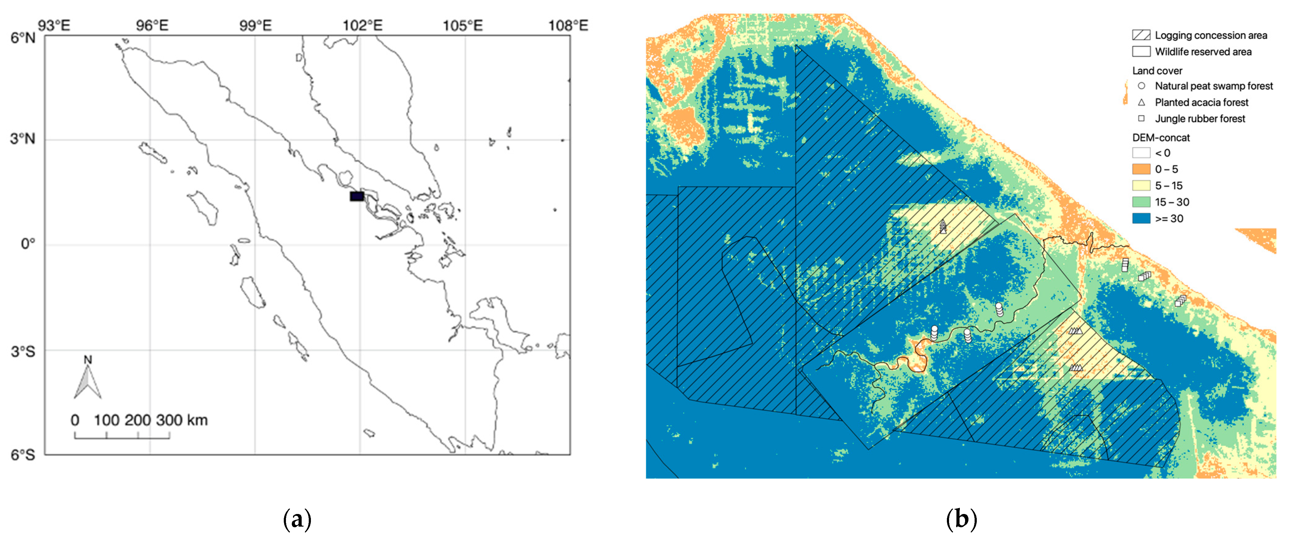
2.1. Study Area

Our study site is in the Bukit Batu area of the Giam Siak Kecil-Bukit Batu Biosphere Reserve in Riau Province on the island of Sumatra in Indonesia (Figure 1). In 1982, peat swamp forests still covered most of this area, but it had been heavily logged by 1993 [31], and half of the area had been transformed to acacia plantation by 2007 [10].
Since some of these artificial forests may be important habitats for some species [32,33], we targeted the following three forest types [34] in this study: (i) natural peat swamp forests (NPF), conserved and managed by the Forestry Department of Riau (Figure 2a); (ii) planted acacia forests (PAF) of Acacia crassicarpa managed by plantation companies (Figure 2b); and (iii) jungle rubber forests (JRF), which are low-maintenance rubber plantations managed by local people (Figure 2c). We targeted the NPF that had already been logged but had preserved complex multilayer structures [7,35], because of the great difficulty in accessing NPF that remained intact.

2.2. Bird Census

We used the dataset of a bird census previously carried out to observe bird occurrence [34] using three survey transects in each land-cover type (NPF1-3, PAF1-3, and JRF1-3), for a total of nine transects (Figure 3). Each transect was 1 km long with four survey points set 250 m apart [36]. The survey was conducted 4 times on each survey point to give 16 surveys per transect and was carried out during October 2011 in NPF and March and May 2011 in JRF and PAF. We used a fixed-radius point-count method. The number and species of individual birds appearing within a 25 m radius of the circular plot were visually and acoustically detected within 20 min. The observation was conducted in the morning (6:00–10:00) and late afternoon (14:00–18:00), when birds are active and easy to observe.
Two out of three bird survey experts (Fujita, Haryadi, and Wijamukti) were involved in each point-count census, to decrease the possibility of observation error. In the ecological field observation, three types of observation errors are common: (a) overlooking species that are present, (b) misidentifying species, and (c) incorrectly estimating abundance [37]. Although the study is based on vegetation survey, the conclusion of Morrison [37] that the use of multiple observers and continual training of observers are useful to reduce observer error could be applied to bird survey to some extent. In our bird survey, multiple observers were involved, and recordings of bird sounds were performed in most of the census to check the bird identification after the survey.
Observed species were then classified into forest-dependent or non-forest-dependent species [34,38]. A species was categorized as a forest-dependent species if the species inhabited primary or secondary forests, and not plantations, scrub, and gardens, according to the descriptions by MacKinnon and Phillips [38]. The species that were not classified as forest-dependent species were categorized as non-forest-dependent species. In addition, threatened species were classified based on the IUCN Red List in 2015 [39] as near-threatened (NT), vulnerable (VU), endangered (EN), and critically endangered (CR). Since species in urgent need of conservation are those associated primarily with native habitats (i.e., NPF), we focused on forest-dependent and threatened species in this paper. Table 1 shows occurrence per census of all the species observed at each habitat. The following analysis used a bird’s occurrence rate (%) of forest-dependent and threatened species, which was calculated by dividing the total occurrence of concerned species by that of all species (Table 2).

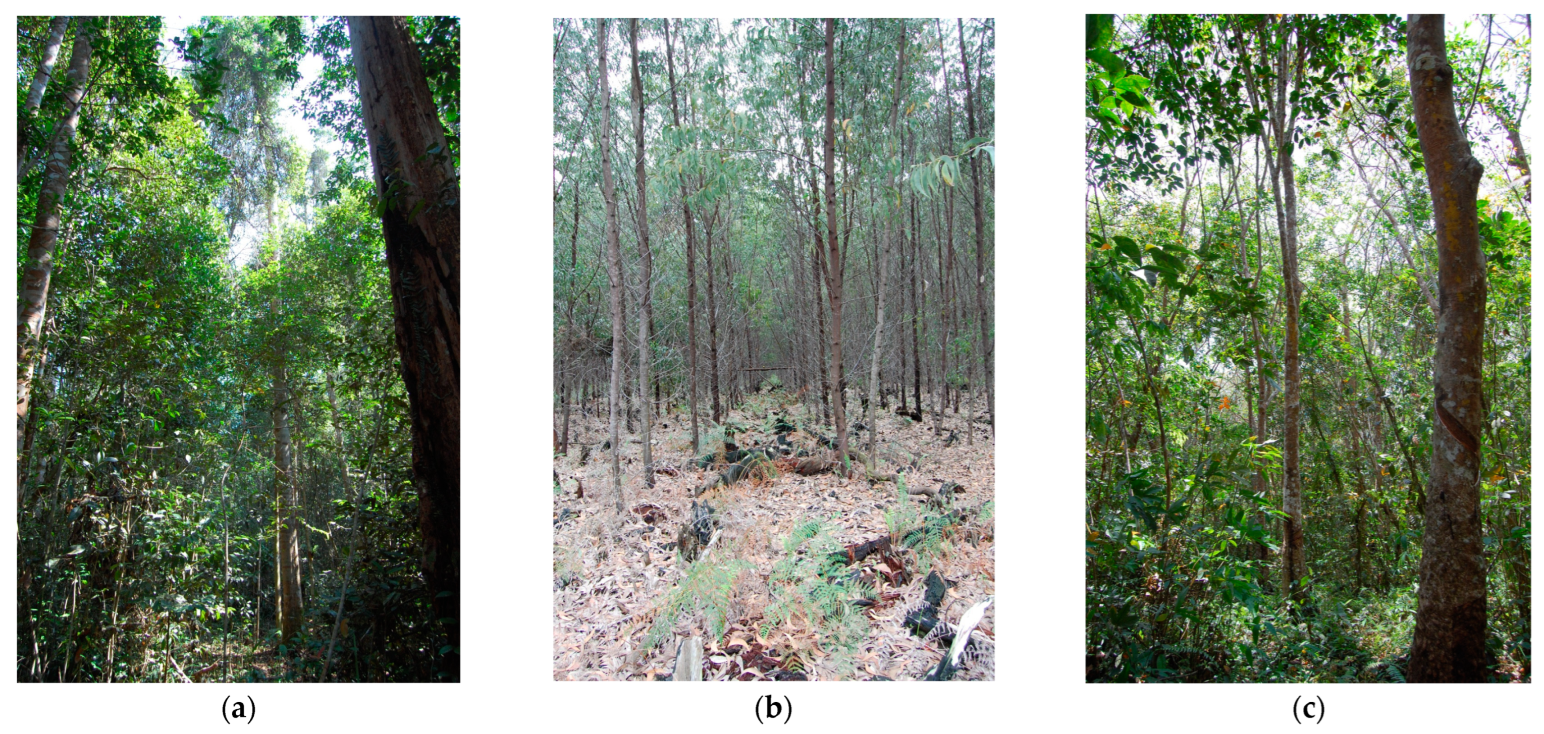
2.3. Field Survey of Forest Layer Structure

Forest layer structure in a 25 m radius of each survey point was observed by assessing vegetation coverage at each forest layer. Since the Braun-Blanquet cover-abundance scale by visual assessment is widely used in ecological studies [40], we employed the method for assessing habitat characteristics [36]. We categorized the forest layers into five layers (<1 m, 1–5 m, 5–10 m, 10–20 m, and 20–30 m) and measured coverage (%) in each of the five layers.
The vegetation in tropical forests typically comprises several layers: (1) forest floor, including herbs, ferns, and mosses; (2) understory, including shrubs and lower trees; (3) upper canopy of dominant trees; and (4) emergent tree layer [41]. Based on the facts that trees greater than 10 m in height formed the canopy layer and the emergent layer was almost absent due to logging activities, we recategorized the layers into three: a forest floor layer less than 1 m, understory layer from 1 m to 10 m, and canopy layer from 10 m to 30 m.
Field survey results are summarized for each transect (Table 2), including the number of censuses, bird occurrence rate, and vegetation coverage. The surveys were conducted for each survey point, and we then averaged values for each transect. However, the vegetation survey was not conducted in NPF3 due to time constraints during fieldwork [34]. Because we summed the observed coverages (%) according to the layer division, some vegetation coverages are greater than 100%. In general, NPF shows multi-story layers with vegetation coverage in all layers, while PAF structure is quite simple, with a forest floor layer and acacia canopy; JRF shows a relatively multilayered structure, although vegetation coverage differs between transects.

2.4. Preprocessing of Microwave Satellite Remote Sensing Data

We used space-borne L-band SAR data acquired by Advanced Land Observing Satellite (ALOS) Phased Array type L-band Synthetic Aperture Radar (PALSAR) with HH/HV/VV/VH polarizations, where H and V refer to horizontal and vertical polarizations, respectively. Two images covering our study site were acquired in an ascending orbit on 31 March 2010 and 16 May 2010, with off-nadir angles of 21.5° and 23.1°, respectively. No quad polarimetric SAR (PolSAR) data were collected in 2011 when most of the ground surveys were conducted.
We first applied absolute radiometric calibration to level 1.1 SAR products [42]. To reduce speckle noise, a moving average filter was then applied to each matrix element using a window size of 2 × 10 (range and azimuth direction, respectively). The PALSAR images have nominal spatial resolutions of 22 m (range direction) and 4.5 m (azimuth direction), meaning that the averaging filter was applied to an area of approximately 45 m × 45 m on the ground. Since local topographic effects can be disregarded, we did not apply radiometric and geometric terrain corrections. As shown in Figure 1b, peat swamp forests are typically located in coastal lowlands and have flat topography; elevation only rises to 20 m at 24.5 km from rivers [5]. Our target forests were less than 1 km from rivers, so they were on flat terrain.
We then calculated covariance and coherency matrices in order to obtain magnitudes of the backscattering coefficient and decomposition powers, which were used in calculation of polarimetric parameters mentioned in Section 3.1. After calculation, we converted each image from a slant range to a ground range and finally registered imagery using the Universal Transverse Mercator (UTM) projection. Ground pixel spacing was set to approximately 25 m, followed by an inverse distance-weighted interpolation with a unit weighting factor.
This satellite data processing was conducted mainly using sentinel application platform (SNAP), which is offered by the European space agency (ESA), and using MATLAB software (version 9.9).

3. Data Analysis

3.1. Polarimetric Parameters Obtained from L-Band SAR Data

We derived the following polarimetric parameters: (1) a backscattering coefficient of sigma naught (σ0) in decibels (dB) for HH, HV, and VV polarizations [43]; (2) polarization ratios (HV/HH, HV/VV, and VV/HH) using the magnitude of the backscattering coefficient, but not dB values converted to a logarithmic scale; (3) decomposition powers of surface (Ps), volume (Pv), double-bounce (Pd), and helix (Pc) scattering, which were normalized by dividing by total power (TP) [30] and are abbreviated as PsTP, PvTP, PdTP, and PcTP; and (4) the decomposition power ratios of Pv/Pd and Pv/Ps, calculated based on the decomposition power.
For PolSAR data analysis, polarimetric power decomposition is widely used [44]. While the three-component decomposition yields surface, double-bounce, and volume scattering [45], higher accuracy is expected—even in forested areas—with a four-component decomposition scheme by adding helix scattering [46,47] as it separates artificial structures from other components as an independent component. The method has been further improved [48] and is known as general four-component scattering power decomposition with unitary transformation (G4U), which was adopted in this analysis.
We averaged each polarimetric parameter (Table 3) over a buffer zone with a 50 m radius constructed around each bird census 1 km transect, assuming uniformity of forest structure within the survey transect. We applied a 50 m radius buffer because pixel spacing itself is 25 m, and there is an inherent positional error between geo-referenced satellite image and survey point data taken by the global positioning system, GPS.

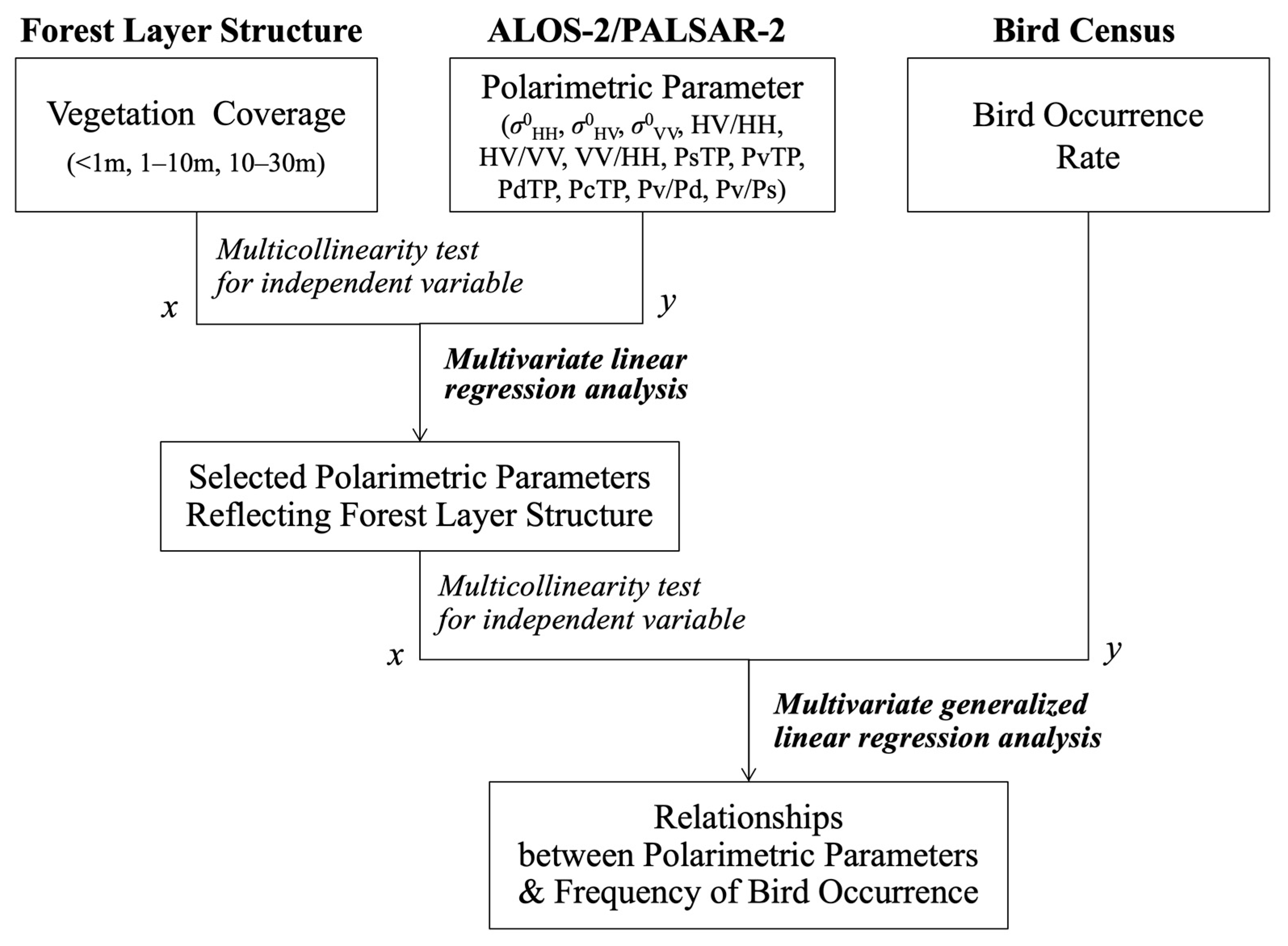
3.2. Statistical Analysis: Polarimetric Parameter Selection and Correlation with Bird Occurrence

We performed the following two statistical analyses, illustrated in a schematic diagram of the analysis procedure (Figure 4), to identify polarimetric parameters representing the forest layer, which would, in turn, indicate bird species richness.
First, we applied multivariate linear regression analysis to explore whether SAR polarimetric parameters reflect forest layer structure. The explanatory variables are the ground-observed vegetation coverage (Table 2) of the three forest layers (<1 m, 1–10 m, and 10–30 m), while the response variables are the SAR polarimetric parameters (Table 3). Multivariate regression analysis requires a minimum sample size of two per independent variable for unbiased estimation [49]. Accordingly, our sample size of eight (NPF3 does not have vegetation survey data) satisfies the minimum criteria of six for three independent variables. Furthermore, high correlation among explanatory variables of multivariate analysis, known as multicollinearity, also negatively impacts the regression coefficient estimation. Therefore, the selection of explanatory variables was performed based on the variance inflation factor (VIF), which is a diagnostic value for testing multicollinearity. The variable with the highest VIF value was repeatedly excluded until all the VIFs for the remaining variables became less than 10 [50]. Then, we undertook multivariate regression analysis of forest layer coverage and SAR polarimetric parameters using explanatory variables not showing multicollinearity. We applied a stepwise forward selection method based on Akaike’s Information Criterion (AIC). The AIC selection finally identified a SAR parameter affected strongly by a forest vegetation layer. In addition, we illustrated scatter plots to gain an intuitive understanding of the relationship between forest layer coverage and each polarimetric parameter.
Next, we used a multivariate generalized linear model (GLM), applying Poisson error distribution and the log link function, to examine the relationship between polarimetric parameters (explanatory variables) and bird occurrence rate (response variables) of forest-dependent and threatened species. The independent variables were limited to polarimetric parameters that showed a stronger correlation with the forest vegetation layer in the previous analysis. In addition, the independent variables having different units were standardized by using z-score normalization to compare calculated regression coefficients. After the VIF multicollinearity test for explanatory variables, we applied a stepwise forward selection method using AIC to discriminate polarimetric parameters with a stronger relationship with bird occurrence rate.

4. Results

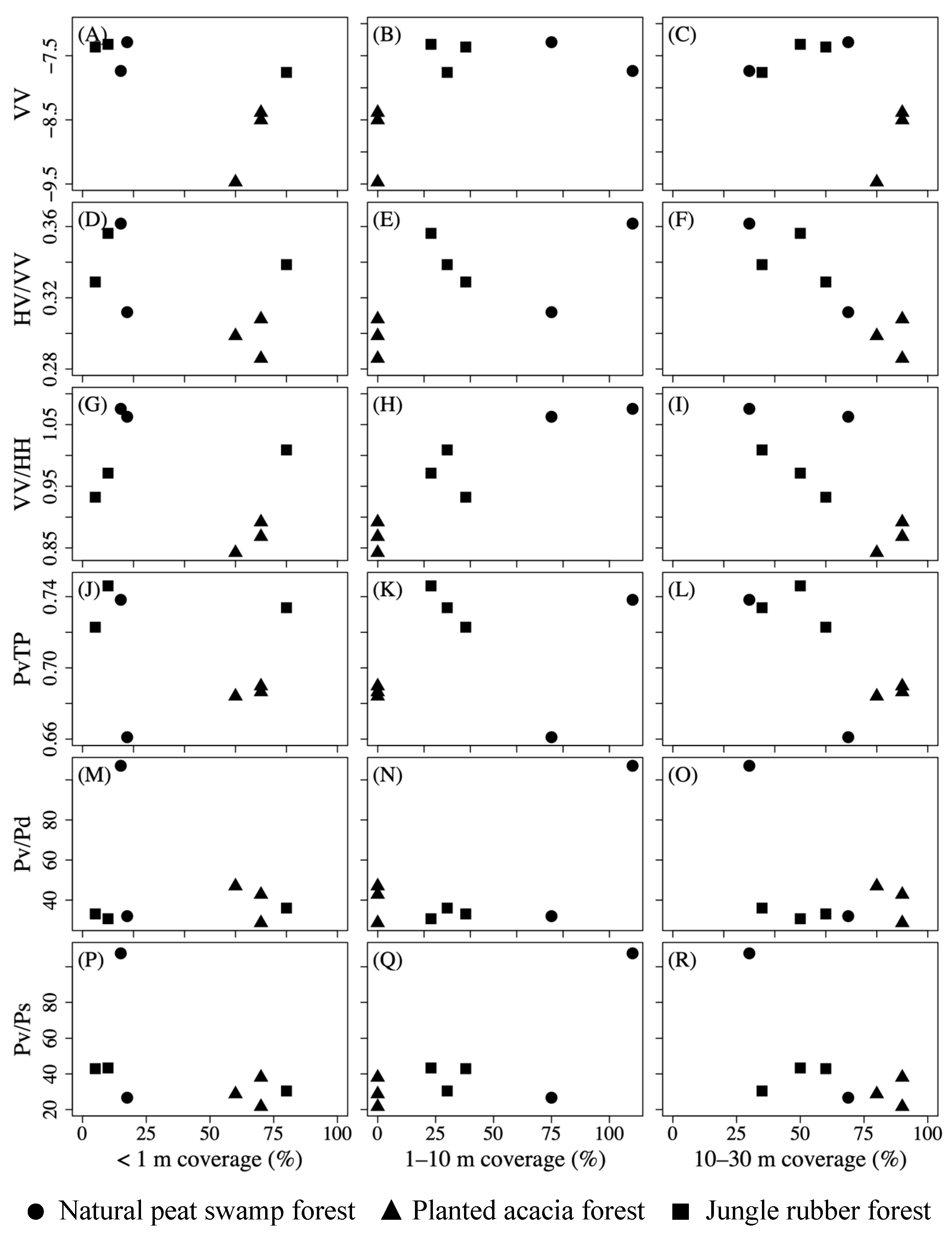
4.1. Polarimetric Parameters Reflecting Forest Layer Structure

Before the regression analysis of vegetation coverage and polarimetric parameters, multicollinearity was tested. The VIF values of 1.64, 2.60, and 1.88 for <1 m, 1–10 m, and 10–30 m, respectively, indicate that there is no multicollinearity among explanatory variables (each VIF value is less than 10). We then analyzed the relationship between vegetation coverage, namely <1 m, 1–10 m, and 10–30 m (Table 2), and each polarimetric parameter from L-band SAR (Table 3). As a result of multivariate linear regression analysis with AIC selection (Table 4), seven polarimetric parameters, σ0VV, HV/HH, VV/HH, PvTP, PcTP, Pv/Pd, and Pv/Ps, show statistical significance (p < 0.10). However, we removed the helix scattering component (PcTP) from the subsequent analysis since it is known to detect artificial structures, which did not exist in our target area. Scatter plots (Figure 5) depict the relationship between coverage in each forest layer (%) and polarimetric parameters (σ0VV, HV/HH, VV/HH, PvTP, Pv/Pd, and Pv/Ps), showing consistency with the statistical analysis (Table 4).
The parameter σ0VV is explained by the forest floor layer (<1 m) with a negative coefficient (Figure 5A). The σ0VV polarization shows a relatively good relationship with the forest floor layer (adj. R2 = 0.343, p = 0.074, respectively). The fact that these parameters are negatively correlated indicates that more scattering of copolarization occurs where the ground surface is scarcely covered by forest floor vegetation. The parameter HV/HH is explained predominantly by 10–30 m (p = 0.005; Figure 5F) and <1 m (p = 0.236; Figure 5D) with greater significance (adj. R2 = 0.819, p = 0.006). On the other hand, VV/HH shows a significant positive correlation only with the middle understory (1–10 m) layer (adj. R2 = 0.778, p = 0.002; Figure 5H), which indicates that VV/HH increases with understory coverage. The parameter PvTP shows a strong correlation with the forest canopy layer (p = 0.014 for 10–30 m, Figure 5L), although other layers were retained as estimates (p = 0.085 for 1–10 m, Figure 5K; p = 0.332 for <1 m, Figure 5J). Although both Pv/Pd and Pv/Ps show a high correlation with 1–10 m (adj. R2 = 0.367 and adj. R2 = 0.474, respectively), Figure 5N,Q depict that the outlier creates the association. Thus, we excluded Pv/Pd and Pv/Ps from the following analysis. Four parameters used for further analysis, σ0VV, HV/HH, VV/HH, and PvTP, were consequently selected as parameters representing the forest layer structure.

4.2. Polarimetric Parameters Correlated with Bird Occurrence

Multicollinearity tests of the four polarimetric parameters (σ0VV, HV/HH, VV/HH, and PvTP) gave VIF values of 96.5, 233.7, 102.2, and 92.8, respectively. Hence, we omitted HV/HH, which had the largest VIF, in recalculating VIF. Since the recalculated VIF values were all less than 10 (1.6, 1.3, and 1.9 for σ0VV, VV/HH, and PvTP, respectively), indicating no multicollinearity, these three polarimetric parameters were subsequently analyzed.
As shown in Table 5, multivariate GLM analysis between three polarimetric parameters and bird occurrence shows that the VV/HH is selected at the highest significance level (p < 0.001) for both forest-dependent and threatened species. Meanwhile, σ0VV is selected at the highest significance (p < 0.001) for threatened species and a lower significance (p = 0.087) for forest-dependent species, and PvTP is selected at the lower significance level (p = 0.092) only for forest-dependent species.
Scatter plots (Figure 6) support the regression analysis results (Table 5) as VV/HH shows a better fit with bird occurrence (Figure 6B,E) than σ0VV does (Figure 6A,D). The goodness of fit in the regression line was assessed by Pseudo R2 statistics [51], indicating clear relationships of σ0VV (Pseudo R2 = 0.294 and 0.378 for forest-dependent and threatened species, respectively) and VV/HH (Pseudo R2 = 0.547 and 0.397 for forest-dependent and threatened species, respectively) to bird occurrence. As can be seen in Figure 6C,F, PvTP shows no significant association (Pseudo R2 = 0.007 and 0.010 for forest-dependent and threatened species, respectively).

5. Discussion

5.1. Mechanisms of L-Band Backscattering against Forest Layer Structure

The L-band SAR evidently enables the detection of the forest layer structure. Our study proves that copolarization scattering of VV contains information about forest floor vegetation. The correlation of σ0VV with forest floor coverage (Table 4 and Figure 5A) agrees well with earlier studies that report strong penetration of L-band copolarizations through the vegetation canopy [52,53,54] and sensitiveness of the VV signal to rough surfaces [54]. When analyzing radar backscatter from the forest floor, we need to consider canopy penetration of the radar, which depends on canopy volume, the presence of canopy gaps, and radar wavelength [53]. Penetration is considered to be sufficient in the targeted forests for the following reasons. Firstly, radar with a smaller incidence angle is less sensitive to crown cover [28]. Our L-band SAR datasets were taken with a relatively small incidence angle of 23°. Secondly, many of the thick trunk trees commonly found in natural forests in our study area had already been removed by logging activities, and trees taller than 30 m are now rare in these forests, resulting in less than 10% emergent layer. Similarly, artificial plantations (JRF and PAF) have relatively thin canopy layers. Although layer thickness is not assessed in our study, it is reasonable to conclude that the L-band VV polarized wave can reach the ground surface through a non-dense canopy in all the forest types to assess the forest floor condition.
The power ratio of VV/HH increases in proportion to understory layer coverage at 1–10 m (adj. R2 = 0.778; Table 4, Figure 5H). It is well known that copolarizations penetrate forest canopy much more effectively than cross-polarizations, and HH and VV signals are most sensitive to trunk-ground structure and rough bare surface, respectively [54]. The HH polarization is mainly generated by trunk-ground double-bounce scattering, increasing with trunk width and the number of trees and decreasing with increasing ground vegetation [53,55]. Therefore, greater understory coverage results in lower HH backscatter and higher VV/HH. This is supported by Singh et al. [56], who found that a ratio of co-polarized waves emphasizes the information of double-bounce scattering from vegetation. The results indicate that the copolarized metric of VV/HH plays an important role in parameterizing the multilayered structure of this forest.
Our results indicate that the canopy layer is explained better by the volume scattering component (Table 4, Figure 5L). It is generally accepted that volume scattering is generated from the canopy layer [53] and increases with vegetation volume. Our results in Table 3 show consistency with this tendency; NPF and JRF show higher σ0HV and PvTP values, and PAF shows lower values, indicating that the vegetation volume is greater in NPF and JRF compared to PAF. Although vegetation volume was not assessed in our study, the scattering power values are consistent with field observations (M. Fujita, personal observation). However, contrary to our expectations and the well-known backscattering effect, the canopy layer coverage (10–30 m) shows a clear negative correlation with volume scattering (PvTP) (Figure 5L). This can possibly be attributed to the decorrelation between canopy extent and volume. Indeed, PAF, which has a lower PvTP value, is characterized by high and relatively uniform canopy coverage of 80–90% (Table 2), as all the trees were planted in the same year. In contrast, NPF and JRF, which have higher PvTP values, are characterized by lower canopy coverage of 30–66% (Table 2). Canopy coverage in natural and low-maintenance planted forests is lower because it does not consider metrics of canopy thickness or overlapping leaves. The facts mentioned above very likely result in a negative correlation between canopy coverage and volume scattering.
Because of the unique property of the L-band signal penetrating the forest canopy, scattering mechanisms are complicated, making image interpretation difficult. Therefore, the statistical approach was used to determine satellite parameters that represent the structure. Our statistical analysis showed reasonable agreement with the previously reported backscatter mechanisms. We then finally conclude that some polarimetric parameters of L-band SAR can be utilized as an indication of the forest layer structure.

5.2. Bird Occurrence Explained by Polarimetric Parameters from L-Band SAR

Possible estimators of bird occurrence can be identified (Table 5): (1) VV/HH, which is positively related to understory vegetation; and (2) σ0VV, which is negatively related to forest floor vegetation. Our analysis indicates that dense understory vegetation results in a higher occurrence of forest-dependent and threatened bird species.
This outcome is deduced from the fact that VV/HH is correlated with an increase in bird occurrences for both the forest-dependent and threatened species (Figure 6B,E and Table 5). As VV/HH values are positively correlated with the understory (1–10 m) vegetation (Figure 5H and Table 4), larger VV/HH values indicate a greater understory layer (Figure 7). Therefore, larger VV/HH values explain the higher occurrence of forest-dependent and threatened species.
This result is implicitly supported by higher bird occurrence with greater σ0VV values (Figure 6A,D), which correlate negatively with forest floor vegetation (Figure 5A and Table 4). Since lower forest floor vegetation is typically formed under conditions of dense upper vegetation, where little sunlight reaches the ground, the inverse relationship between the understory and floor vegetation is consistent (Figure 7). Indeed, NPF and JRF are characterized by lower forest floor coverage and higher understory coverage (Table 2). However, some results show slight contradictions in terms of coverage. Transects, especially in PAF, with greater forest floor (<1 m) vegetation show greater canopy coverage (10–30 m) (Table 2). This result is most likely because Acacia crassicarpa plantations have lower leaf density than is found in natural vegetation. Therefore, the stand has better light conditions than would be expected from the canopy coverage; hence, dense forest floor vegetation was observed (M. Fujita, personal observation). Lower canopy coverage in the NPF, in contrast, does not necessarily mean an open canopy since the sum of understory and canopy coverage was high enough (>100%) to block sunlight from reaching the forest floor (Figure 2, Table 2).

5.3. Feasibility of Bird Diversity Monitoring by Microwave SAR

The positive deviation of NPF data points from the regression lines (Figure 6A,B,D,E) shows that NPF has more species than expected from the regression. This is possibly because of the increased plant species diversity in natural forests, which was not accounted for in our study. NPF comprises richer plant species diversity in comparison with planted forests. Increased plant diversity creates many resources (e.g., food, nesting materials, and places) for birds, thereby increasing bird diversity [57]. Although our method using forest layer structure can provide a good predictor of bird occurrence, other parameters that explain plant diversity are needed, especially for natural vegetation, which has richer plant diversity.
Even with the limitations in detecting plant diversity mentioned above, L-band SAR data are still useful for evaluating bird assemblages via forest layer structure estimation. As an active optical remote sensing method, LiDAR is used to measure tree height and three-dimensional information at very fine resolution for remote sensing observations of bird diversity [13,16,17,58,59,60,61], sometimes by combining different types of sensors [62,63]. On the other hand, LiDAR data remains very costly because its main platform is an airplane [29]. TomoSAR, which is an advanced synthetic aperture radar (SAR) technique, uses SAR interferometry (InSAR) technology. As it requires scenes that are taken from slightly different satellite positions with high scene coherency [64,65], achieved solely by single-pass airborne SAR, particularly over forest areas, data availability remains spatially and temporally limited. Some studies aiming at broad monitoring take the approach of using passive optical remote sensing [66,67,68,69]. However, because visible-to-near infrared light is physically scattered by canopy leaves and cannot penetrate deeper, the widely used optical sensors are unable to detect forest layer structure.
For these reasons, PolSAR is expected to play an important role in remote monitoring of biodiversity, provided that the forest canopy is not too dense to allow L-band microwave penetration. If for some reason, the targeted forest has canopy gaps, radar can penetrate deeper into the forest to capture more information beneath the forest canopy. On the other hand, a dense canopy with more natural vegetation tends to reduce penetration because radar penetration depends on canopy volume; hence, it is difficult to observe the internal structure of such forests even with longer wavelength of L-band SAR.
It should be noted that our analysis only deals with a small sample size in a short sampling period. This is primarily due to the time constraints and budget shortage as the fieldwork requires huge effort. As a result, survey results contain uncertainty, and this study was unable to conduct external validation, which is the process of confirming the validity of the prediction model on others. Therefore, the results must be considered carefully before being applied widely to other habitat types. Although a more comprehensive study is required to widen the implications of our findings, our results clearly demonstrate the potential of applying SAR polarimetric parameters to assess bird occurrence and diversity through the estimation of vegetation structure in tropical peat swamps.

6. Conclusions

We succeeded in identifying the potential of using L-band SAR data to assess bird diversity through the estimation of forest layer structure. Forest floor, middle understory, and canopy vegetation layer are explained by SAR polarimetric parameters, some of which show a significant correlation with the occurrence of the forest-dependent and threatened bird species. However, the SAR data analysis indicated that forest layer structure alone is not enough to predict bird diversity in natural forests, where plant species richness is higher than in plantations. As plant diversity seems difficult to detect with SAR signals, incorporating other remote sensing techniques to detect plant diversity should be investigated in the future. Nevertheless, this study offers a new interpretation and application of L-band SAR data for conducting large-scale and long-term assessments of bird diversity. By applying this method, it would be possible to offer a quick diagnosis of biodiversity using satellite data, particularly in tropical peatland that is exposed to rapid biodiversity loss and is difficult to access. Then, the result could be used to determine the areas with high priority of biodiversity conservation.

Author Contributions

Conceptualization, S.K. and M.S.F.; methodology, S.K. and M.S.F.; formal analysis, S.K.; investigation, M.S.F., D.S.H., A.M., M.I. and S.S.; data curation, M.S.F.; writing—original draft preparation, S.K.; writing—review and editing, S.K. and M.S.F.; supervision, Y.O. All authors have read and agreed to the published version of the manuscript.

Funding

This work was supported by JSPS KAKENHI Grant Number JP 18K11626, and JSPS Global COE Program “In Search of Sustainable Humanosphere in Asia”. ALOS/PALSAR data used in this study were provided by Japan Aerospace Exploration Agency (JAXA).

Acknowledgments

We greatly thank Canecio Munoz, Sinar Mas Forestry, for his kind assistance and providing accommodation during our fieldwork at PT. Bukit Batu Hutani Alam and PT. Sakato Pratama Makmur. We also thank the Forest Department and BBKSDA Riau for permission to conduct our research in the Bukit Batu Wildlife Reserve. Satrio Wijamukti greatly helped identify bird species during bird censuses.

Conflicts of Interest

The authors declare no conflict of interest.

References

  1. Sodhi, N.S.; Brook, B.W. Southeast Asian Biodiversity in Crisis; Cambridge University Press: Cambridge, UK, 2006. [Google Scholar]
  2. Sodhi, N.S.; Koh, L.P.; Brook, B.W.; Ng, P.K. Southeast Asian biodiversity: An impending disaster. Trends Ecol. Evol. 2004, 19, 654–660. [Google Scholar] [PubMed]
  3. Sodhi, N.S.; Lee, T.M.; Koh, L.P.; Brook, B.W. A meta-analysis of the impact of anthropogenic forest disturbance on Southeast Asia’s biotas. Biotropica 2009, 41, 103–109. [Google Scholar]
  4. Andriesse, J. Nature and Management of Tropical Peat Soils; Food & Agriculture Org.: Rome, Italy, 1988. [Google Scholar]
  5. Page, S.; Rieley, J.; Shotyk, Ø.; Weiss, D. Interdependence of peat and vegetation in a tropical peat swamp forest. In Changes and Disturbance in Tropical Rainforest in South-East Asia; World Scientific: Singapore, 1999; pp. 161–173. [Google Scholar]
  6. Cheyne, S.M.; Macdonald, D.W. Wild felid diversity and activity patterns in Sabangau peat-swamp forest, Indonesian Borneo. Oryx 2011, 45, 119–124. [Google Scholar]
  7. Posa, M.R.C. Peat swamp forest avifauna of Central Kalimantan, Indonesia: Effects of habitat loss and degradation. Biol. Conserv. 2011, 144, 2548–2556. [Google Scholar]
  8. Giam, X.; Clements, G.R.; Aziz, S.A.; Chong, K.Y.; Miettinen, J. Rethinking the ‘back to wilderness’ concept for Sundaland’s forests. Biol. Conserv. 2011, 144, 3149–3152. [Google Scholar] [CrossRef]
  9. Corlett, R.T. The Ecology of Tropical East Asia; Oxford University Press: Oxford, UK, 2014. [Google Scholar]
  10. Uryu, Y.; Mott, C.; Foead, N.; Yulianto, K.; Budiman, A.; Setiabudi; Takakai, F.; Nursamsu; Sunarto; Purastuti, E.; et al. Deforestation, Forest Degradation, Biodiversity Loss and CO2 Emissions in Riau, Sumatra, Indonesia; WWF Indonesia Technical Report: Jakarta, Indonesia, 2008. [Google Scholar]
  11. Proença, V.; Martin, L.J.; Pereira, H.M.; Fernandez, M.; McRae, L.; Belnap, J.; Böhm, M.; Brummitt, N.; García-Moreno, J.; Gregory, R.D. Global biodiversity monitoring: From data sources to essential biodiversity variables. Biol. Conserv. 2017, 213, 256–263. [Google Scholar]
  12. Nagendra, H.; Lucas, R.; Honrado, J.P.; Jongman, R.H.G.; Tarantino, C.; Adamo, M.; Mairota, P. Remote sensing for conservation monitoring: Assessing protected areas, habitat extent, habitat condition, species diversity, and threats. Ecol. Indic. 2013, 33, 45–59. [Google Scholar] [CrossRef]
  13. Petrou, Z.I.; Manakos, I.; Stathaki, T. Remote sensing for biodiversity monitoring: A review of methods for biodiversity indicator extraction and assessment of progress towards international targets. Biodivers. Conserv. 2015, 24, 2333–2363. [Google Scholar] [CrossRef]
  14. Mulatu, K.A.; Mora, B.; Kooistra, L.; Herold, M. Biodiversity monitoring in changing tropical forests: A review of approaches and new opportunities. Remote Sens. 2017, 9, 1059. [Google Scholar] [CrossRef]
  15. Munro, N.T.; Fischer, J.; Barrett, G.; Wood, J.; Leavesley, A.; Lindenmayer, D.B. Bird’s Response to Revegetation of Different Structure and Floristics-Are “Restoration Plantings” Restoring Bird Communities? Restor. Ecol. 2011, 19, 223–235. [Google Scholar] [CrossRef]
  16. Wallis, C.I.B.; Paulsch, D.; Zeilinger, J.; Silva, B.; Fernandez, G.F.C.; Brandl, R.; Farwig, N.; Bendix, J. Contrasting performance of Lidar and optical texture models in predicting avian diversity in a tropical mountain forest (vol 174, pg 223, 2016). Remote Sens. Environ. 2016, 178, 223. [Google Scholar] [CrossRef]
  17. Weisberg, P.J.; Dilts, T.E.; Becker, M.E.; Young, J.S.; Wong-Kone, D.C.; Newton, W.E.; Ammon, E.M. Guild-specific responses of avian species richness to LiDAR-derived habitat heterogeneity. Acta Oecol. 2014, 59, 72–83. [Google Scholar] [CrossRef]
  18. Erdelen, M. Bird communities and vegetation structure: I. Correlations and comparisons of simple and diversity indices. Oecologia 1984, 61, 277–284. [Google Scholar] [PubMed]
  19. Karr, J.R.; Roth, R.R. Vegetation structure and avian diversity in several New World areas. Am. Nat. 1971, 105, 423–435. [Google Scholar] [CrossRef]
  20. Díaz, I.A.; Armesto, J.J.; Reid, S.; Sieving, K.E.; Willson, M.F. Linking forest structure and composition: Avian diversity in successional forests of Chiloé Island, Chile. Biol. Conserv. 2005, 123, 91–101. [Google Scholar]
  21. Zellweger, F.; Baltensweiler, A.; Ginzler, C.; Roth, T.; Braunisch, V.; Bugmann, H.; Bollmann, K. Environmental predictors of species richness in forest landscapes: Abiotic factors versus vegetation structure. J. Biogeogr. 2016, 43, 1080–1090. [Google Scholar] [CrossRef]
  22. El Moussawi, I.; Ho Tong Minh, D.; Baghdadi, N.; Abdallah, C.; Jomaah, J.; Strauss, O.; Lavalle, M.; Ngo, Y.-N. Monitoring tropical forest structure using SAR tomography at L-and P-band. Remote Sens. 2019, 11, 1934. [Google Scholar] [CrossRef]
  23. Joshi, N.; Mitchard, E.; Schumacher, J.; Johannsen, V.; Saatchi, S.; Fensholt, R. L-Band SAR Backscatter Related to Forest Cover, Height and Aboveground Biomass at Multiple Spatial Scales across Denmark. Remote Sens. 2015, 7, 4442–4472. [Google Scholar] [CrossRef]
  24. Lucas, R.M.; Mitchell, A.L.; Rosenqvist, A.; Proisy, C.; Melius, A.; Ticehurst, C. The potential of L-band SAR for quantifying mangrove characteristics and change: Case studies from the tropics. Aquat. Conserv. 2007, 17, 245–264. [Google Scholar] [CrossRef]
  25. Robinson, C.; Saatchi, S.; Neumann, M.; Gillespie, T. Impacts of Spatial Variability on Aboveground Biomass Estimation from L-Band Radar in a Temperate Forest. Remote Sens. 2013, 5, 1001–1023. [Google Scholar] [CrossRef]
  26. Carreiras, J.M.B.; Vasconcelos, M.J.; Lucas, R.M. Understanding the relationship between aboveground biomass and ALOS PALSAR data in the forests of Guinea-Bissau (West Africa). Remote Sens. Environ. 2012, 121, 426–442. [Google Scholar] [CrossRef]
  27. Cartus, O.; Santoro, M.; Kellndorfer, J. Mapping forest aboveground biomass in the Northeastern United States with ALOS PALSAR dual-polarization L-band. Remote Sens. Environ. 2012, 124, 466–478. [Google Scholar] [CrossRef]
  28. Imhoff, M.L.; Sisk, T.D.; Milne, A.; Morgan, G.; Orr, T. Remotely sensed indicators of habitat heterogeneity: Use of synthetic aperture radar in mapping vegetation structure and bird habitat. Remote Sens. Environ. 1997, 60, 217–227. [Google Scholar] [CrossRef]
  29. Betbeder, J.; Hubert-Moy, L.; Burel, F.; Corgne, S.; Baudry, J. Assessing ecological habitat structure from local to landscape scales using synthetic aperture radar. Ecol. Indic. 2015, 52, 545–557. [Google Scholar] [CrossRef]
  30. Kobayashi, S.; Omura, Y.; Sanga-Ngoie, K.; Yamaguchi, Y.; Widyorini, R.; Fujita, M.S.; Supriadi, B.; Kawai, S. Yearly Variation of Acacia Plantation Forests Obtained by Polarimetric Analysis of ALOS PALSAR Data. IEEE J. Sel. Top. Appl. Earth Obs. Remote Sens. 2015, 8, 5294–5304. [Google Scholar] [CrossRef]
  31. Mizuno, K.; Fujita, M.S.; Kawai, S. Catastrophe and Regeneration in Indonesia’s Peatlands: Ecology, Economy and Society; NUS Press: Singapore, 2016; Volume 15. [Google Scholar]
  32. Fujita, M.S.; Prawiradilaga, D.M.; Yoshimura, T. Roles of fragmented and logged forests for bird communities in industrial Acacia mangium plantations in Indonesia. Ecol. Res. 2014, 29, 741–755. [Google Scholar]
  33. Barlow, J.; Gardner, T.A.; Araujo, I.S.; Avila-Pires, T.C.; Bonaldo, A.B.; Costa, J.E.; Esposito, M.C.; Ferreira, L.V.; Hawes, J.; Hernandez, M.M.; et al. Quantifying the biodiversity value of tropical primary, secondary, and plantation forests. Proc. Natl. Acad. Sci. USA 2007, 104, 18555–18560. [Google Scholar] [CrossRef] [PubMed]
  34. Fujita, M.S.; Samejima, H.; Haryadi, D.S.; Muhammad, A.; Irham, M.; Shiodera, S. Low conservation value of converted habitat for avifauna in tropical peatland on Sumatra, Indonesia. Ecol. Res. 2016, 31, 275–285. [Google Scholar] [CrossRef]
  35. Edwards, D.P.; Larsen, T.H.; Docherty, T.D.; Ansell, F.A.; Hsu, W.W.; Derhé, M.A.; Hamer, K.C.; Wilcove, D.S. Degraded lands worth protecting: The biological importance of Southeast Asia’s repeatedly logged forests. Proc. R. Soc. Lond. B Biol. Sci. 2011, 278, 82–90. [Google Scholar]
  36. Ralph, C.J. Handbook of Field Methods for Monitoring Landbirds; Pacific Southwest Research Station: Albany, CA, USA, 1993; Volume 144. [Google Scholar]
  37. Morrison, L.W. Observer error in vegetation surveys: A review. J. Plant Ecol. 2016, 9, 367–379. [Google Scholar]
  38. MacKinnon, J.R.; Phillipps, K. A Field Guide to the Birds of Borneo, Sumatra, Java, and Bali, the Greater Sunda Islands; Oxford University Press: Oxford, UK, 1993. [Google Scholar]
  39. IUCN. The IUCN Red List of Threatened Species. Version 2015-4. Available online: http://www.iucnredlist.org (accessed on 28 November 2015).
  40. Wikum, D.A.; Shanholtzer, G.F. Application of the Braun-Blanquet cover-abundance scale for vegetation analysis in land development studies. Environ. Manag. 1978, 2, 323–329. [Google Scholar] [CrossRef]
  41. Richards, P.W.; Tansley, A.G.; Watt, A.S. The Recording of Structure, Life Form and Flora of Tropical Forest Communities as a Basis for Their Classification. J. Ecol. 1940, 28, 224–239. [Google Scholar] [CrossRef]
  42. Small, D. Flattening Gamma: Radiometric Terrain Correction for SAR Imagery. IEEE Trans. Geosci. Remote Sens. 2011, 49, 3081–3093. [Google Scholar] [CrossRef]
  43. Shimada, M.; Isoguchi, O.; Tadono, T.; Isono, K. PALSAR Radiometric and Geometric Calibration. IEEE Trans. Geosci. Remote Sens. 2009, 47, 3915–3932. [Google Scholar] [CrossRef]
  44. Richards, J.A. Remote Sensing with Imaging Radar; Springer: Berlin/Heidelberg, Germany, 2009. [Google Scholar]
  45. Freeman, A.; Durden, S.L. A three-component scattering model for polarimetric SAR data. IEEE Trans. Geosci. Remote Sens. 1998, 36, 963–973. [Google Scholar] [CrossRef]
  46. Yamaguchi, Y.; Moriyama, T.; Ishido, M.; Yamada, H. Four-component scattering model for polarimetric SAR image decomposition. IEEE Trans. Geosci. Remote Sens. 2005, 43, 1699–1706. [Google Scholar] [CrossRef]
  47. Yamaguchi, Y.; Sato, A.; Boerner, W.M.; Sato, R.; Yamada, H. Four-Component Scattering Power Decomposition With Rotation of Coherency Matrix. IEEE Trans. Geosci. Remote Sens. 2011, 49, 2251–2258. [Google Scholar] [CrossRef]
  48. Singh, G.; Yamaguchi, Y.; Park, S.E. General Four-Component Scattering Power Decomposition With Unitary Transformation of Coherency Matrix. IEEE Trans. Geosci. Remote Sens. 2013, 51, 3014–3022. [Google Scholar] [CrossRef]
  49. Austin, P.C.; Steyerberg, E.W. The number of subjects per variable required in linear regression analyses. J. Clin. Epidemiol. 2015, 68, 627–636. [Google Scholar] [CrossRef]
  50. Montgomery, D.C.; Peck, E.A.; Vining, G.G. Introduction to Linear Regression Analysis; John Wiley & Sons: Hoboken, NJ, USA, 2012; Volume 821. [Google Scholar]
  51. Hardin, J.W.; Hardin, J.W.; Hilbe, J.M.; Hilbe, J. Generalized Linear Models and Extensions, 2nd ed.; Taylor & Francis: Abingdon, UK, 2007. [Google Scholar]
  52. Ottinger, M.; Kuenzer, C. Spaceborne L-Band Synthetic Aperture Radar Data for Geoscientific Analyses in Coastal Land Applications: A Review. Remote Sens. 2020, 12, 2228. [Google Scholar] [CrossRef]
  53. Henderson, F.M.; Ryerson, R.A.; Lewis, A.J.; Photogrammetry, A.S.f.; Sensing, R. Principles and Applications of Imaging Radar; Wiley: Hoboken, NJ, USA, 1998. [Google Scholar]
  54. Flores-Anderson, A.I.; Herndon, K.E.; Thapa, R.B.; Cherrington, E. The SAR Handbook: Comprehensive Methodologies for Forest Monitoring and Biomass Estimation; SERVIR Global Science. National Space Science and Technology Center: Huntsville, AL, USA, 2019. [Google Scholar]
  55. Pope, K.O.; Rey-Benayas, J.M.; Paris, J.F. Radar remote sensing of forest and wetland ecosystems in the Central American tropics. Remote Sens. Environ. 1994, 48, 205–219. [Google Scholar]
  56. Singh, G.; Venkataraman, G.; Yamaguchi, Y.; Park, S.-E. Capability assessment of fully polarimetric ALOS–PALSAR data for discriminating wet snow from other scattering types in mountainous regions. IEEE Trans. Geosci. Remote Sens. 2013, 52, 1177–1196. [Google Scholar] [CrossRef]
  57. Márquez, A.L.; Real, R.; Vargas, J.M. Dependence of broad-scale geographical variation in fleshy-fruited plant species richness on disperser bird species richness. Glob. Ecol. Biogeogr. 2004, 13, 295–304. [Google Scholar]
  58. Boelman, N.T.; Holbrook, J.D.; Greaves, H.E.; Krause, J.S.; Chmura, H.E.; Magney, T.S.; Perez, J.H.; Eitel, J.U.H.; Gough, L.; Vierling, K.T.; et al. Airborne laser scanning and spectral remote sensing give a bird’s eye perspective on arctic tundra breeding habitat at multiple spatial scales. Remote Sens. Environ. 2016, 184, 337–349. [Google Scholar] [CrossRef]
  59. Goetz, S.; Steinberg, D.; Dubayah, R.; Blair, B. Laser remote sensing of canopy habitat heterogeneity as a predictor of bird species richness in an eastern temperate forest, USA. Remote Sens. Environ. 2007, 108, 254–263. [Google Scholar] [CrossRef]
  60. Vogeler, J.C.; Hudak, A.T.; Vierling, L.A.; Evans, J.; Green, P.; Vierling, K.I.T. Terrain and vegetation structural influences on local avian species richness in two mixed-conifer forests. Remote Sens. Environ. 2014, 147, 13–22. [Google Scholar] [CrossRef]
  61. Bergen, K.M.; Goetz, S.J.; Dubayah, R.O.; Henebry, G.M.; Hunsaker, C.T.; Imhoff, M.L.; Nelson, R.F.; Parker, G.G.; Radeloff, V.C. Remote sensing of vegetation 3-D structure for biodiversity and habitat: Review and implications for lidar and radar spaceborne missions. J. Geophys. Res.-Biogeosci. 2009, 114. [Google Scholar] [CrossRef]
  62. Singh, M.; Friess, D.A.; Vilela, B.; Alban, J.D.T.D.; Monzon, A.K.V.; Veridiano, R.K.A.; Tumaneng, R.D. Spatial relationships between above-ground biomass and bird species biodiversity in Palawan, Philippines. PLoS ONE 2017, 12, e0186742. [Google Scholar]
  63. Singh, M.; Tokola, T.; Hou, Z.; Notarnicola, C. Remote sensing-based landscape indicators for the evaluation of threatened-bird habitats in a tropical forest. Ecol. Evol. 2017, 7, 4552–4567. [Google Scholar]
  64. Shimada, M. Imaging from Spaceborne and Airborne SARs, Calibration, and Applications; CRC Press: Boca Raton, FL, USA, 2018. [Google Scholar]
  65. Tello, M.; Cazcarra-Bes, V.; Pardini, M.; Papathanassiou, K. Forest structure characterization from SAR tomography at L-band. IEEE J. Sel. Top. Appl. Earth Obs. Remote Sens. 2018, 11, 3402–3414. [Google Scholar] [CrossRef]
  66. Wu, J.; Chen, B.; Reynolds, G.; Xie, J.; Liang, S.; O’Brien, M.J.; Hector, A. Monitoring tropical forest degradation and restoration with satellite remote sensing: A test using Sabah Biodiversity Experiment. In Advances in Ecological Research; Elsevier: Amsterdam, The Netherlands, 2020; Volume 62, pp. 117–146. [Google Scholar]
  67. Ribeiro, I.; Proença, V.; Serra, P.; Palma, J.; Domingo-Marimon, C.; Pons, X.; Domingos, T. Remotely sensed indicators and open-access biodiversity data to assess bird diversity patterns in Mediterranean rural landscapes. Sci. Rep. 2019, 9, 6826. [Google Scholar] [PubMed]
  68. Suttidate, N.; Hobi, M.L.; Pidgeon, A.M.; Round, P.D.; Coops, N.C.; Helmers, D.P.; Keuler, N.S.; Dubinin, M.; Bateman, B.L.; Radeloff, V.C. Tropical bird species richness is strongly associated with patterns of primary productivity captured by the Dynamic Habitat Indices. Remote Sens. Environ. 2019, 232, 111306. [Google Scholar] [CrossRef]
  69. Wallis, C.I.; Brehm, G.; Donoso, D.A.; Fiedler, K.; Homeier, J.; Paulsch, D.; Süßenbach, D.; Tiede, Y.; Brandl, R.; Farwig, N. Remote sensing improves prediction of tropical montane species diversity but performance differs among taxa. Ecol. Indic. 2017, 83, 538–549. [Google Scholar] [CrossRef]
Figure 1. (a) Location of the study site (indicated by a small black square) in Sumatra, Indonesia. (b) Location of survey transects: natural peat swamp forests (NPF) shown by circles, planted acacia forests (PAF) by triangles, and jungle rubber forests (JRF) by rectangles. Bukit Batu Wildlife Reserve is shown in a rectangle along the Bukit Batu River. Acacia plantations are shown in the area with diagonal lines, where logging operation is permitted and managed by plantation companies named PT Bukit Batu Hutani Alam and PT Sakato Paratama Makmuri.
Remotesensing 15 00947 g001
Figure 2. Forest cover types in the study area: (a) natural peat swamp forests (NPF), (b) planted acacia forests (PAF), and (c) jungle rubber forests (JRF).
Remotesensing 15 00947 g002
Figure 3. Three transects established on each land cover: natural peat swamp forests (NPF), planted acacia forests (PAF), and jungle rubber forests (JRF). Four survey points were on a 1 km each survey transect. The background is an RGB color composite image using different polarizations (R = HH; G = HV; B = VV).
Remotesensing 15 00947 g003
Figure 4. Analysis flow chart.
Remotesensing 15 00947 g004
Figure 5. Scatter plots of vegetation coverage (%) and polarimetric parameters that show significance association (Table 4). The plots on the left represent vegetation coverage of less than 1 m on the x-axis, the central column of plots represents vegetation coverage between 1 m and 10 m, and the right-hand plots represent vegetation coverage between 10 m and 30 m. The y-axis shows each polarimetric parameter: (AC) σ0VV, (DF) HV/HH, (GI) VV/HH, (JL) PvTP, (MO) Pv/Pd, and (PR) Pv/Ps. The circle, triangle, and square points correspond to surveyed data on natural peat swamp forest (NPF), planted acacia forest (PAF), and Jungle rubber forest (JRF), respectively.
Remotesensing 15 00947 g005
Figure 6. Bird occurrence rate (response variable) in relation to L-band polarimetric parameters (explanatory variable) for forest-dependent and threatened species. Solid line indicates logarithmic regression line: (AC) forest dependent species with the explanatory variable of σ0VV, VV/HH, and PvTP, respectively. (DF) threatened species with the explanatory variable of σ0VV, VV/HH, and PvTP, respectively. The circle, triangle, and square points correspond to data on natural peat swamp forest (NPF), planted acacia forest (PAF), and Jungle rubber forest (JRF), respectively.
Remotesensing 15 00947 g006
Figure 7. Schematic diagram of the inverse relationship between understory and forest floor vegetation. Higher understory coverage is represented by increased VV/HH, which positively relates to bird occurrence rate. On the contrary, lower forest floor coverage is presented by increased VV signals which also positively relate to bird occurrence.
Remotesensing 15 00947 g007
Table 1. List of forest-dependent species occurrence observed in each habitat type: natural peat swamp forests (NPF), planted acacia forests (PAF), and jungle rubber forests (JRF). The numbers indicate mean occurrence per census per habitat type. Abbreviations for IUCN status: CR, critically endangered; NT, near-threatened; LC, least concern.
English NameScientific NameAuthorIUCN (2015)Occurrence/Census
NPFPAFJRF
Rufous PiculetSasia abnormis(Temminck, CJ 1825)LC0.0240.0000.000
Red-throated BarbetMegalaima
mystacophanos
(Temminck, CJ 1824)NT0.0000.0000.021
Black HornbillAnthracoceros
malayanus
(Raffles, TS 1822)NT0.0000.0000.083
Helmeted HornbillBuceros vigil(Pennant, T 1781)CR0.0000.0420.000
Diard’s TrogonHarpactes diardii(Temminck, CJ 1832)NT0.0240.0000.000
Drongo-cuckooSurniculus
lugubris
(Horsfield, T 1821)LC0.0240.0000.000
Blue-crowned Hanging-parrotLoriculus galgulus(Linnaeus, C 1758)LC0.0710.0000.000
Thick-billed Green-pigeonTreron curvirostra(Gmelin, JF 1789)LC0.0000.0000.104
Black-and-yellow BroadbillEurylaimus ochromalus(Raffles, TS 1822)NT0.0950.0000.000
Asian Fairy-bluebirdIrena puella(Latham, J 1790)LC0.0240.0000.000
Greater Green LeafbirdChloropsis
sonnerati
(Jardine, W; Selby, PJ 1827)LC0.0240.0000.000
Lesser Green LeafbirdChloropsis
cyanopogon
(Temminck, CJ 1830)NT0.1430.0000.000
Black-winged Flycatcher-shrikeHemipus
hirundinaceus
(Temminck, CJ 1822)LC0.0000.0000.417
Greater Racket-tailed DrongoDicrurus
paradiseus
(Linnaeus, C 1766)LC0.0480.0000.000
Black-naped MonarchHypothymis azurea(Boddaert, P 1783)LC0.0240.0000.000
Indian Paradise-flycatcherTerpsiphone
paradisi
(Linnaeus, C 1758)LC0.0240.0000.000
Rufous-winged PhilentomaPhilentoma
pyrhopterum
(Temminck, CJ 1836)LC0.0240.0000.000
Grey-chested Jungle-flycatcherRhinomyias
umbratilis
(Strickland, HE 1849)NT0.1670.0000.000
White-rumped ShamaCopsychus
malabaricus
(Scopoli, GA 1786)LC0.0000.0000.021
Common Hill MynaGracula religiosa(Linnaeus, C 1758)LC0.0000.0000.083
Spectacled BulbulPycnonotus erythropthalmos(Hume, AO 1878)LC0.4520.0000.000
Streaked BulbulIxos malaccensis(Blyth, E 1845)NT0.0240.0000.000
Ferruginous BabblerTrichastoma bicolor(Lesson, RP 1839)LC0.0240.0000.000
Black-throated BabblerStachyris
nigricollis
(Temminck, CJ 1836)NT0.0710.0000.104
Chestnut-rumped BabblerStachyris maculata(Temminck, CJ 1836)NT0.0950.0000.000
Fluffy-backed Tit-babblerMacronous ptilosus(Jardine, W; Selby, PJ 1835)NT0.1190.0000.000
Scarlet-breasted FlowerpeckerPrionochilus
thoracicus
(Temminck, CJ 1836)NT0.0950.0000.000
Table 2. Number of bird censuses, bird occurrence rate of forest-dependent and threatened species, and vegetation coverage in each forest layer on each survey transect. No vegetation survey was conducted in NPF3.
TransectNumber of CensusBird Occurrence Rate (%)Vegetation Coverage (%)
Forest
Dependent
Threatened <1 m1–10 m10–30 m
NPF11841.627.31511030
21652.832.1187569
3835.030.0N/AN/AN/A
PAF1162.66.470090
2160.00.070090
3160.00.060080
JRF1161.78.653860
21611.016.5102350
31613.814.4803035
Table 3. SAR polarimetric parameters for each survey transect. Digital Number (DN) values within a 50 m radius buffer around each survey transect were averaged.
σ0HHσ0HVσ0VVHV/
HH
HV/
VV
VV/
HH
PsTPPvTPPdTPPcTPPv/PdPv/Ps
NPF1−7.917−12.584−7.7370.3620.3421.0760.0950.7380.0890.078107.0107.5
2−7.384−12.654−7.2880.3120.3031.0630.1530.6610.1110.07532.0026.66
3−7.392−12.474−7.7800.3200.3520.9360.1160.7080.0970.07941.1546.20
PAF1−7.784−13.027−8.3860.3080.3540.8920.1150.6900.1230.07228.6538.06
2−7.760−13.324−8.5020.2860.3420.8680.1470.6860.0960.07042.8121.60
3−8.492−14.022−9.4710.2990.3700.8420.1410.6840.1060.07047.0028.72
JRF1−6.872−11.858−7.3640.3290.3660.9320.0820.7230.1180.07633.1242.96
2−7.098−11.711−7.3210.3560.3730.9710.0820.7460.0950.07630.7243.30
3−7.658−12.536−7.7600.3390.3411.0090.1050.7340.0880.07336.0330.44
Table 4. Results of multivariate linear regression analysis between forest layer structures (explanatory variable) and polarimetric parameters from L-band SAR data (response variables). AIC-selected variables are shown with estimates, p-values are within parentheses, and a hyphen “-” indicates variables not selected in AIC stepwise selection. The overall adequacy of the model was assessed using adj. R2 and p-value. Significance levels are denoted as follows: “•” is p < 0.100, “*” is p < 0.050, and “**” is p < 0.010. “○” in front of parameter names indicates those selected for the next analysis.
Response
Variable (y)
Estimates and p-Value (in Parentheses) of
Selected Explanatory Variables (x)
Model
Fitting
Polarimetric
Parameter
<1 m1–10 m10–30 mAdj. R2
(p-Value)
σ0HH−0.962
(0.112)
--0.259
(0.112)
σ0HV−1.753
(0.116)
−0.990
(0.323)
−2.090
(0.174)
0.422
(0.180)
σ0VV−1.587
(0.074 •)
--0.343
(0.074 •)
HV/HH−0.020
(0.236)
-−0.095
(0.005 **)
0.819
(0.006 **)
HV/VV−0.041
(0.205)
−0.073
(0.053 •)
−0.060
(0.197)
0.387
(0.201)
VV/HH 0.199
(0.002 **)
0.778
(0.002 **)
PsTP0.052
(0.177)
0.058
(0.144)
0.118
(0.063 •)
0.476
(0.150)
PvTP−0.029
(0.322)
−0.059
(0.085 •)
−0.158
(0.014 *)
0.708
(0.049 *)
PdTP−0.017
(0.282)
-0.045
(0.060 •)
0.632
(0.140)
PcTP−0.007
(0.007 **)
-−0.007
(0.024 *)
0.870
(0.002 **)
Pv/Pd-44.17
(0.065 •)
-0.367
(0.065 •)
Pv/Ps-51.12
(0.035 *)
-0.474
(0.035 •)
Table 5. The results of multivariate generalized linear model (GLM) analysis between the polarimetric parameters (explanatory variables) and bird occurrence rate of forest-dependent and threatened species (response variables). Estimates and p-values (in parentheses) were shown for AIC-selected variables. A hyphen “-” indicates variables not selected. Significance levels are denoted as follows: “•” is p < 0.100, and “***” is p < 0.001.
Response Variable (y)Estimates and p-Value (in Parentheses) of
Selected Explanatory Variables (x)
Bird Occurrence Rateσ0VVVV/HHPvTP
Forest-dependent0.318
(0.087 •)
0.885
(<0.001 ***)
−0.116
(0.092 •)
Threatened0.600
(<0.001 ***)
0.460
(<0.001 ***)
-
Disclaimer/Publisher’s Note: The statements, opinions and data contained in all publications are solely those of the individual author(s) and contributor(s) and not of MDPI and/or the editor(s). MDPI and/or the editor(s) disclaim responsibility for any injury to people or property resulting from any ideas, methods, instructions or products referred to in the content.

