An Unmixing-Based Multi-Attention GAN for Unsupervised Hyperspectral and Multispectral Image Fusion

Abstract

Hyperspectral images (HSI) frequently have inadequate spatial resolution, which hinders numerous applications for the images. High resolution multispectral image (MSI) has been fused with HSI to reconstruct images with both high spatial and high spectral resolutions. In this paper, we propose a generative adversarial network (GAN)-based unsupervised HSI-MSI fusion network. In the generator, two coupled autoencoder nets decompose HSI and MSI into endmembers and abundances for fusing high resolution HSI through the linear mixing model. The two autoencoder nets are connected by a degradation-generation (DG) block, which further improves the accuracy of the reconstruction. Additionally, a coordinate multi-attention net (CMAN) is designed to extract more detailed features from the input. Driven by the joint loss function, the proposed method is straightforward and easy to execute in an end-to-end training manner. The experimental results demonstrate that the proposed strategy outperforms the state-of-art methods.

1. Introduction

Hyperspectral remote sensing is a multi-dimensional information acquisition technology combining imaging and spectral technology, which can simultaneously obtain two-dimensional spatial and one-dimensional spectral information targets. Each pixel of a hyperspectral image (HSI) has its own spectrum with high spectral resolution, which reflects the physical nature of the captured object. Therefore, hyperspectral imagers have been developed for environment classification [1,2,3,4], target detection [5,6,7,8], feature extraction and dimensionality reduction [9,10,11,12], spectral unmixing [13,14,15], and so on. However, for a hyperspectral imaging system, there is trade-off between spatial and spectral resolution due to limited sensor size and imaging performance. The spatial resolution of HSIs is lower than that of panchromatic images or multispectral images (MSIs). The low spatial resolution severely limits the performance of HSIs in applications. In order to enhance the spatial resolution of HSI, fusion-based methods have been proposed to merge HSI with a relative high-resolution (HR) MSI. The existing fusion methods can be categorized in three types: extensions of pan-sharpening methods [16,17,18,19], bayesian-based approaches [20,21,22,23], and spectral unmixing based methods [24,25,26,27,28,29,30,31,32,33,34,35].

In the first category, pan-sharpening image fusion algorithms are extended to fusing low-resolution (LR) HSI and HR-MSI. For example, Gomez et al. [16] first extended a wavelet-based pan-sharpening algorithm to fuse HSI with MSI. Zhang et al. [17] introduced a 3D wavelet transform for HSI-MSI fusion. Chen et al. [18] divided the HSI into several regions and fused the HSI and MSI in each region using a pan-sharpening method. Aiazzi et al. [19] proposed a component substitution fusion method, which took the spectral response function (SRF) as part of the model.

In the second category, Eismann et al. [20] proposed a Bayesian fusion method based on a stochastic mixing model of the underlying spectral content to achieve resolution enhancement. Wei et al. [21] proposed a variational-based fusion method by incorporating a sparse regularization using trained dictionaries and optimization the problem through the split augmented Lagrangian shrinkage algorithm. Simões et al. [22] formulated the fusion problem as a minimization of a convex objection containing two quadratic terms and an edge-preserving term. Akhtar et al. [23] proposed a nonparametric Bayesian sparse coding strategy, which first inferred the probability distributions of the material spectra and then computed the sparse codes of the high-resolution image.

Methods in the third category usually assume that the HSI is composed of a series of pure spectra (named as endmembers) with corresponding proportion (named as abundance) maps. Therefore, matrix decomposition [24,25,26] and tensor factorization algorithms [27] have been used to decompose both LR-HSI and HR-MSI into endmembers and abundance maps to generate HR-HSI. For example, Kawakami et al. [24] introduced a matrix factorization algorithm to estimate the endmember-basis of the HSI and fuse it with a RGB image. In Refs [25,26], coupled non-negative matrix fraction (CNMF) had been used to estimate endmembers and abundances for HSI-MSI fusion. Dian et al. [27] proposed a non-local sparse tensor decomposition approach to transform the fusion problem as the estimation of dictionaries in three modes and corresponding core tensors.

In recent years, deep learning methods have been presented and successfully applied in the field of computer vision. Since the deep learning methods have great ability to extract embedded features and represent complex nonlinear mapping, they have been widely used for various remote sensing image procedures, including HSI super-resolution. The thought of HSI fusion based on deep learning can be divided into pan-sharpening [28] and HSI-MSI fusion [29,30,31,32,33,34,35]. For example, Dian et al. [28] proposed a deep HSI sharpening method which used priors learnt via CCN-based residual learning. Recently, some unified image fusion frameworks such as U2Fusion [36] and SwinFusion [37] have been proposed for various fusion issues, including multi-modal, multi-exposure tasks. These frameworks might be modified and utilized for pan-sharpening. The related works about HSI-MSI are detailed in Section 2.

In this paper, a novel unsupervised multi-attention GAN is proposed to solve the HSI–MSI fusion problem with unknown spectral response function (SRF) and point spread function (PSF). Based on the linear unmixing theory, two autoencoders and one constraint network are jointly coupled in the proposed generator net to reconstruction HR-HSI. The model offers an end-to-end unsupervised learning strategy, which is driven by a joint-loss function, to obtain the desired outcome. The main contributions of this study can be summarized as follows.

• An unsupervised GAN, which contains one generator network and two discriminator networks, is developed for HSI-MSI fusion based on the degradation model and the spectral unmixing model. The experiments conducted on four data sets demonstrate that the proposed method outperforms state-of-the-art methods.
• In the generator net, two streams of autoencoders are jointly connected through a degradation-generation (DG) block to perform spectral unmixing and image fusion. The endmembers of DG block are made up of one convolution layer’s parameters that are shared by two autoencoder networks. Also, in order to increase the consistency of these networks, a learnt PSF layer acts as a bridge connecting the low- and high-resolution abundances.
• Our encoder network adopts an attention module called coordinate multi-attention net (CMAN) to extract deeper features from the input data, which consists of a pyramid coordinate channel attention module and a non-local spatial attention module. The channel attention module is factorized into two parallel feature encoding strings to alleviate the inter-positional information among spectral channels.

This article is organized as follows. Section 2 briefly reviews the deep-learning-based HSI-MSI fusion methods and some attention modules. Section 3 describes the degradation relationships between HR-HSI, LR-HSI, and HR-MSI based on the linear spectral mixing model. Section 4 details the proposed generative adversarial network (GAN) framework including the network architecture of generator and discriminator, the structure of the attention module and the loss functions. Section 5 includes the ablation experiments and comparison experiments. Finally, conclusions of our work are drawn in Section 6.

2. Related Works

2.1. Deep Leaning (DL) HSI-MSI Fusion Methods

DL HSI-MSI fusion methods can be divided into two types, one is based on the degradation models [29,30,31,32] and another is based on the spectral mixing model [33,34,35]. In the first category, the fusion networks were constructed to reconstruct desired HR-HSI by using the observation models to depict the spatial degradation relationship between HR-HSI and LR-HSI, as well as the spectral degradation relationship between HR-HSI and HR-MSI. For example, Han et al. [29] present a multi-scale spatial and spectral fusion network for HSI-RGB fusion. Yang et al. [30] proposed a fusion network to extract features from LR-HSI and HR-MSI, and a spatial attention network to recover the high frequency details. Xiao et al. [31] proposed a physical-based GAN, which used the degradation model to generate spatial and spectral degraded images for the discriminators. The GAN used a multiscale residual channel attention fusion module and a residual spatial attention fusion module for fusion. Liu et al. [32] construct an unsupervised multi-attention-guided network, which includes a multi-attention encoding network for extracting sematic features of MSI and a multiscale feature guided network as a regularizer.

In the second category, the networks perform spectral unmixing on LR-HSI and HR-MSI based on the linear mixing model to extract spectral bases and high resolution spatial information for HR-HSI fusion. Qu et al. [33] presented an unsupervised encoder-decoder architecture which used a sparse Dirichlet constraint. Zheng et al. [34] proposed an unsupervised coupled network which consists of autoencoders to extract spectral information from the LR-HSI and spatial–contextual information from the HR-MSI. Yao et al. [35] proposed a coupled convolution autoencoder network which implanted a cross-attention module to transfer the spectral and spatial information between two branches. A closed-loop spatial-spectral consistency regularization was employed in the network to achieve local optimum.

Inspired by the above works, an unsupervised GAN network is developed by incorporating the degradation models with the spectral mixing model, in order to associate the HR-HSI with both the LR-HSI and the HR-MSI. The proposed network has the ability to learn the spatial and spectral degradation across LR-HSI and HR-MSI in an adaptive manner.

2.2. Attention Mechanisms

Recently, attention mechanisms have been deployed for boosting the performance of various deep learning networks in computer vision tasks. Hu [38] designed the squeeze-and-excitation (SE) block to model interdependencies between channels, which could bring notable improvement in performance of CNNs on classification tasks. Sanghyun [39] presented a convolutional block attention module (CBAM) which sequentially exploited the inter-channel and inter-spatial relationships of features, and demonstrated the performance in various applications, i.e., image classification, visualization and object detection. Fu [40] proposed a dual attention network (DANet) for scene segmentation by introducing the position attention module and a channel attention module to capture global dependencies in the spatial and channel dimensions. Zhang [41] proposed an efficient pyramid squeeze attention network (EPSANet) to extract multi-scale spatial information and the cross-dimension channel information, and verified the effectiveness on computer vision task in image classification and object detection.

In this work, in order to more effectively extract spatial-spectral information from HSI and MSI for the fusion task, a multi-attention module that consists of a pyramid channel attention and a global spatial attention is present.

3. Problem Formulation

The HSI–MSI fusion problem is to estimate the HR-HSI datacube, which has both high spectral and high spatial resolution and is denoted as $\mathbf{Y}\in {\mathbb{R}}^{M\times N\times L}$, where M, and N are the spatial dimensions, while L is the number of spectral bands. Similarly, an LR-HSI is denoted as ${\mathbf{X}}_{\mathrm{s}}\in {\mathbb{R}}^{m\times n\times L}$, where m and n are the width and height of ${\mathbf{X}}_{\mathrm{s}}$. And an MSI datacube with high spatial resolution is denoted as ${\mathbf{X}}_{\mathrm{m}}\in {\mathbb{R}}^{M\times N\times l}$, where l is the number of spectral bands in ${\mathbf{X}}_{\mathrm{m}}$, and $l=3$ when an RGB image is employed as the MSI data. To simplify the mathematical derivation, we unfold these 3-D datacubes to 2-D matrices as $\mathbf{Y}\in {\mathbb{R}}^{MN\times L}$, ${\mathbf{X}}_{\mathrm{s}}\in {\mathbb{R}}^{mn\times L}$, ${\mathbf{X}}_{\mathrm{m}}\in {\mathbb{R}}^{MN\times l}$, respectively.

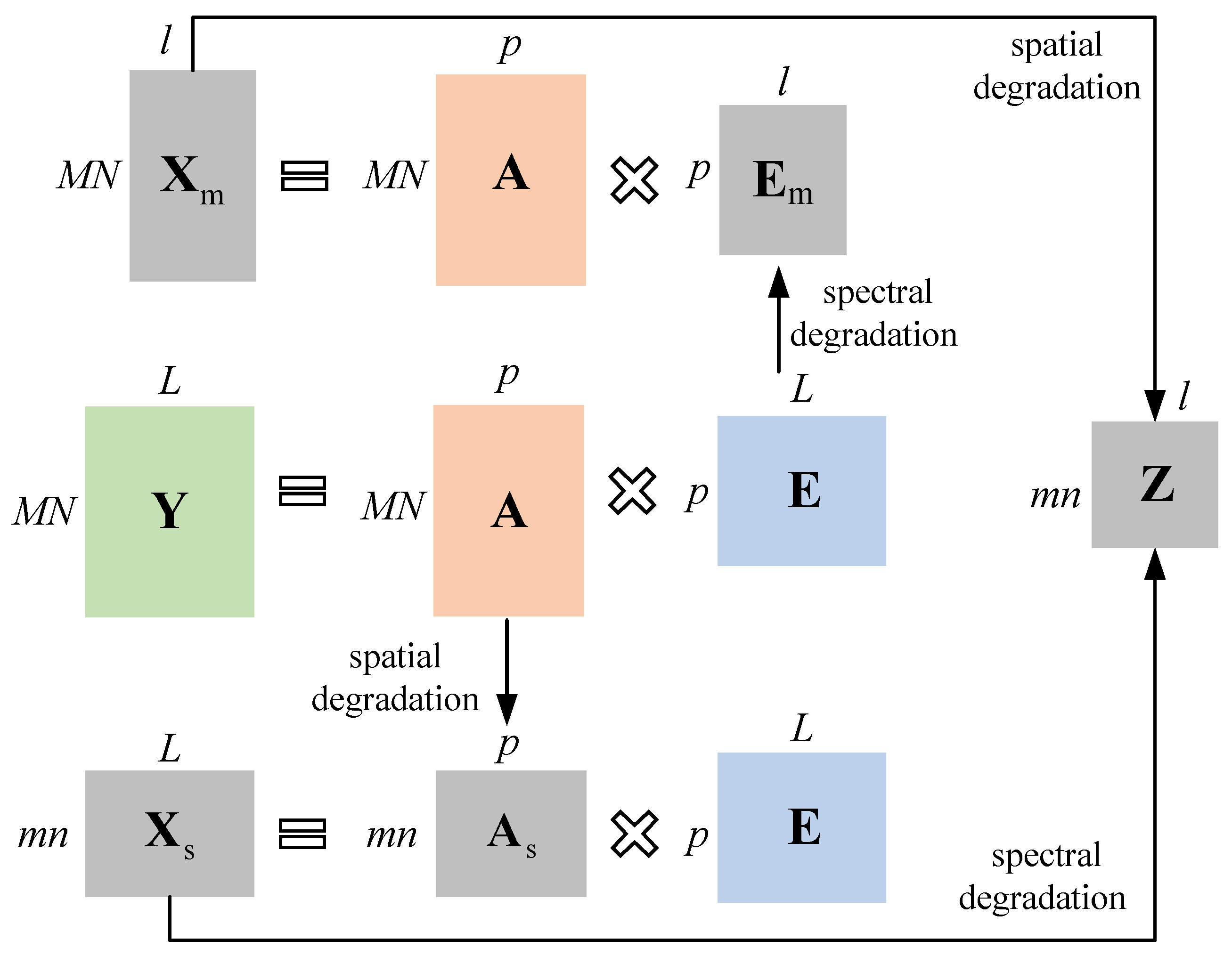
The relationships among ${\mathbf{X}}_{\mathrm{s}}$, ${\mathbf{X}}_{\mathrm{m}}$ and $\mathbf{Y}$ are illustrated in Figure 1. According to the linear mixing model (LMM), each pixel of the HSI is assumed to be a linear combination of a set of pure spectral bases called endmembers. The coefficient of each endmember is called abundance. The HR-HSI $\mathbf{Y}$ can be described as,

$$\mathbf{Y}=\mathbf{AE}$$

(1)

where p is the number of endmembers, the $j^{th}$ column of abundance matrix $\mathbf{A}\in {\mathbb{R}}^{MN\times p}$ consists of columns representing mixing coefficients $a_{ij}$ of the $j^{th}$ endmember at the $i^{th}$ pixel, and the endmember matrix $\mathbf{E}\in {\mathbb{R}}^{p\times L}$ is made up of p endmembers with L spectral bands.

The LR-HSI ${\mathbf{X}}_{\mathrm{s}}$ can also be expressed as a linear combination of the same endmembers $\mathbf{E}$ of $\mathbf{Y}$ as following equation,

$${\mathbf{X}}_{\mathrm{s}}={\mathbf{A}}_{\mathrm{s}}\mathbf{E}$$

(2)

where the matrix ${\mathbf{A}}_{\mathrm{s}}\in {\mathbb{R}}^{mn\times p}$ consists of the coefficients $a_{ij}^{\mathrm{s}}$ of low spatial resolution.

Similarly, the HR-MSI data ${\mathbf{X}}_{\mathrm{m}}$ is given by,

$${\mathbf{X}}_{\mathrm{m}}=\mathbf{A}{\mathbf{E}}_{\mathrm{m}}$$

(3)

where the matrix ${\mathbf{E}}_{\mathrm{m}}\in {\mathbb{R}}^{p\times l}$ is made up of p endmembers with l spectral bands.

The abundance coefficients should satisfy the sum-to-one and nonnegative constraints given by following the respective equations,

$$\sum _{j=1}^p{a}_{ij}=1,\forall ij$$

(4)

$$a_{ij}\ge 0,\forall ij$$

(5)

The spectral bases of endmembers should also satisfy the nonnegative property, which is given by,

$$0\le e_{ij}\le 1,\forall kj$$

(6)

where $e_{kj}$ is the element representing the $k^{th}$ band of the $j^{th}$ endmember.

The LR-HSI ${\mathbf{X}}_{\mathrm{s}}$ can be considered as a spatially degraded version of HR-HSI $\mathbf{Y}$ as,

$${\mathbf{X}}_{\mathrm{s}}=\mathbf{SY}=\mathbf{SAE}$$

(7)

where the matrix $\mathbf{S}\in {\mathbb{R}}^{nm\times MN}$ is the degradation matrix representing the spatial blurring and downsampling operation on $\mathbf{Y}$. Meanwhile, the HR-MSI ${\mathbf{X}}_{\mathrm{m}}$ can be noted as a spectrally degraded version of $\mathbf{Y}$,

$${\mathbf{X}}_m=\mathbf{YR}=\mathbf{AER}$$

(8)

where the spectral degradation matrix $\mathbf{R}\in {\mathbb{R}}^{L\times l}$ is determined by the SRF, which describes the spectral degradation mapping from HSI to MSI. Comparing Equations (1) and (7), it is obvious that the LR-HSI ${\mathbf{X}}_{\mathrm{s}}$ preserves the fine spectral information, which is highly consistent with the target spectral endmembers matrix $\mathbf{E}$. Meanwhile, Equations (1) and (8) also illustrate that the HR-MSI provides detailed spatial contextual information, which is highly correlated with high spatial resolution abundance matrix $\mathbf{A}$. The key point of the HSI–MSI fusion problem is to estimate $\mathbf{E}$ and $\mathbf{A}$ from ${\mathbf{X}}_{\mathrm{s}}$ and ${\mathbf{X}}_{\mathrm{m}}$, respectively, for reconstructing $\mathbf{Y}$.

Furthermore, the ideal LR-MSI $\mathbf{Z}\in {\mathbb{R}}^{mn\times l}$ can either be expressed as a spectrally degraded version of ${\mathbf{X}}_{\mathrm{s}}$ or a spatially degraded version of ${\mathbf{X}}_{\mathrm{m}}$, respectively,

$$\mathbf{Z}={\mathbf{X}}_{\mathrm{s}}\mathbf{R}=\mathbf{S}{\mathbf{X}}_m$$

(9)

This is added in the model as a consistency constraint of the network.

4. Proposed Method

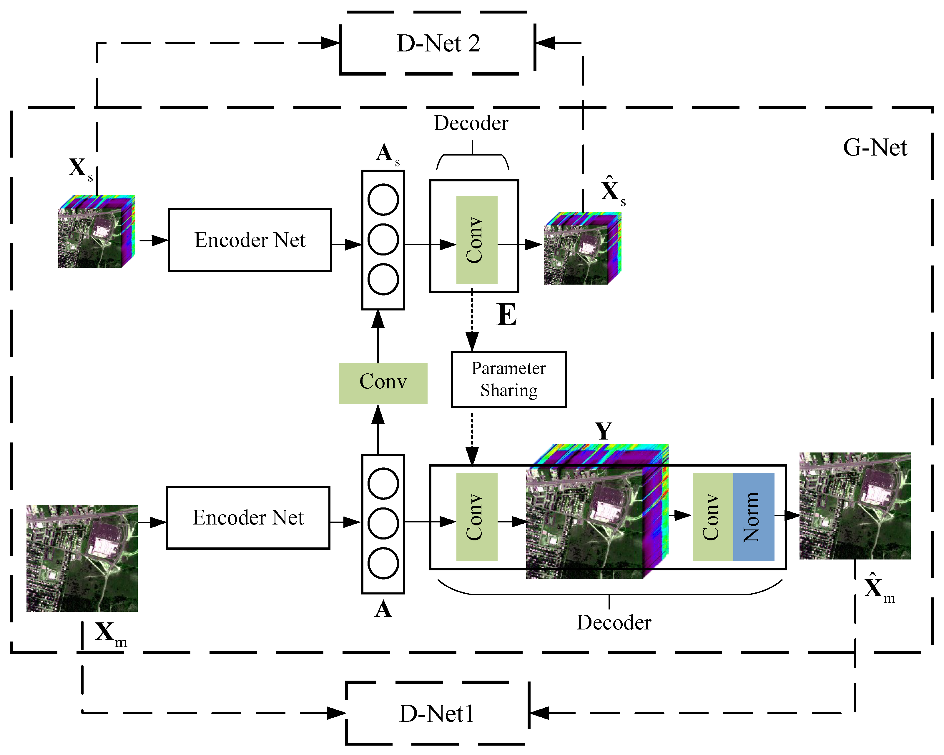
In this paper, we propose a GAN that consists of one generator network (G-Net) and two discriminator networks (D-Net1 and D-Net2), which is based on the models described in Section 4. The whole architecture of the adversarial training is shown in Figure 2. The HR-HSI ${\mathbf{X}}_{\mathrm{s}}$ and LR-MSI ${\mathbf{X}}_{\mathrm{m}}$ are fed and processed in the separated network streams as 3D data without unfolding.

The generator network employs two streams of autoencoder-decoder networks to perform spectral unmixing and data reconstruction. The discriminator nets are employed to extract multi-dimensional features of the input and output from generator networks to obtain the corresponding authenticity probability. A joint loss function incorporated with multiple constraints of the entire network is also presented.

4.1. Generator Network

As shown in Figure 3, the G-net is composed of two main autoencoder networks (AENet1 and AENet2), which are correlated with each other by sharing endmembers. The desired HR-HSI $\mathbf{Y}$ is embedded in one layer of the decoder in the AENet2 as a hidden variable.

The AENet1 is designed to learn the LR-HSI identity function ${\mathcal{G}}_1\left({\mathbf{X}}_{\mathrm{s}}\right)={\hat{\mathbf{X}}}_{\mathrm{s}}^a$. The endmembers $\mathbf{E}$ and abundances ${\mathbf{A}}_s$ are extracted from the input LR-HSI ${\mathbf{X}}_{\mathrm{s}}$ by the AENet1. The encoder module is designed to learn a nonlinear mapping $f_{en}(·)$ which transforms the input ${\mathbf{X}}_{\mathrm{s}}$ to its abundances ${\mathbf{A}}_{\mathrm{s}}^{\mathrm{a}}$ as in following equation,

$${\mathbf{A}}_{\mathrm{s}}^{\mathrm{a}}=f_{en}\left({\mathbf{X}}_{\mathrm{s}}\right).$$

(10)

The overall structure of the encoder is shown in Figure 3. It consists of a 3 × 3 convolution layer followed by a ReLU layer, three cascaded residual blocks (ResBlock) and CMAN blocks, and a 1 × 1 convolution layer. The detailed description of CMAN is in Section 4.3.

The decoder $f_{de}(·)$ reconstructs data ${\widehat{\mathbf{X}}}_{\mathrm{s}}^{\mathrm{a}}$ from ${\mathbf{A}}_{\mathrm{s}}^{\mathrm{a}}$, and its function is noted as,

$${\widehat{\mathbf{X}}}_{\mathrm{s}}^a=f_{de}(\mathbf{E},{\mathbf{A}}_{\mathrm{s}}^{\mathrm{a}})=f_{de}(\mathbf{E},f_{en}\left({\mathbf{X}}_{\mathrm{s}}\right))={\mathcal{G}}_1\left({\mathbf{X}}_{\mathrm{s}}\right).$$

(11)

Meanwhile, the AENet2 is designed to learn the HR-MSI identity function ${\mathcal{G}}_2\left({\mathbf{X}}_{\mathrm{m}}\right)={\widehat{\mathbf{X}}}_{\mathrm{m}}$. The encoder structure of the AENet2 is the same as AENet1, it can transform ${\mathbf{X}}_{\mathrm{m}}$ to the HR abundance matrix $\mathbf{A}$ by following equation,

$$\mathbf{A}=f_{en}\left({\mathbf{X}}_m\right)$$

(12)

The decoder $h_{de}(·)$ of AENet2 is different from that of AENet1, and the function is given as,

$${\widehat{\mathbf{X}}}_{\mathrm{m}}=h_{de}(\mathbf{E},\mathbf{A})=h_{de}(\mathbf{E},f_{en}\left({\mathbf{X}}_m\right))={\mathcal{G}}_2\left({\mathbf{X}}_{\mathrm{m}}\right)$$

(13)

The decoder $h_{de}(·)$ consists of two parts, a convolution layer $f_{de}(·)$ which contains the parameters of the endmember matrix $\mathbf{E}$ shared by AENet1, and a spectral degradation module which adaptively learns the spectral response function $SRF(·)$. The decoder $f_{de}(·)$ generates the desired HR-HSI $\widehat{\mathbf{Y}}=f_{de}\left(\mathbf{A}\right)$, while $SRF(·)$ transform $\widehat{\mathbf{Y}}$ to HR-MSI ${\widehat{\mathbf{X}}}_{\mathrm{m}}$. The relationship is given as the following equation,

$${\widehat{\mathbf{X}}}_{\mathrm{m}}=SRF\left(\widehat{\mathbf{Y}}\right)=SRF\left(f_{de}(\mathbf{E},f_{en}\left({\mathbf{X}}_m\right))\right)={\mathcal{G}}_2\left({\mathbf{X}}_{\mathrm{m}}\right)$$

(14)

The function $SRF(·)$ represents the spectral downsampling from HSI to MSI, and it can be defined as,

$${\varphi }_i=\frac{{\int }_{{\lambda }_{i1}}^{{\lambda }_{i2}}\rho \left(\lambda \right)\epsilon \left(\lambda \right)d\lambda }{{\int }_{{\lambda }_{i1}}^{{\lambda }_{i2}}\rho \left(\lambda \right)d\lambda }$$

(15)

where ${\varphi }_i$ is the spectral radiance of the ith band of the MSI data, [${\lambda }_{i1}$, ${\lambda }_{i2}$] is the wavelength range of the ith band, $\rho$ is the spectral response of the MSI sensor, and $\epsilon$ is the spectral radiance of the HSI data. In order to implement the SRF function in the neural network, a convolution layer and a normalization layer are employed to adaptively learn the numerator and denominator of Equation (15), respectively.

Furthermore, as show in Figure 3, the AENet1 and AENet2 are not only connected by sharing the endmember $\mathbf{E}$, but also connected through a DG block. As given by the hyperspectral linear unmixing model given in Equations (1) and (2), $\mathbf{Y}$ and ${\mathbf{X}}_{\mathrm{s}}$ are composed of the same endmember matrix $\mathbf{E}$. Meanwhile, a low-resolution abundance ${\mathbf{A}}_{\mathrm{s}}^{\mathrm{b}}$ can be generated by applying a convolution layer to perform spatial degradation $d(·)$, and ${\mathbf{A}}_{\mathrm{s}}^{\mathrm{b}}=d\left(\mathbf{A}\right)$. Therefore, in the DG block, we can acquire another LR-HSI data ${\widehat{\mathbf{X}}}_{\mathrm{s}}^{\mathrm{b}}$ from $\mathbf{E}$ and $\mathbf{A}$, by using the same decoding function of AENet1,

$${\widehat{\mathbf{X}}}_{\mathrm{s}}^{\mathrm{b}}=f_{de}(\mathbf{E},{\mathbf{A}}_{\mathrm{s}}^{\mathrm{b}})=f_{de}(\mathbf{E},d\left(\mathbf{A}\right))$$

(16)

The generated ${\widehat{\mathbf{X}}}_{\mathrm{s}}^{\mathrm{b}}$ is another approximation of input LR-HSI ${\mathbf{X}}_{\mathrm{s}}$.

In addition, the spectral degradation module is shared to generate LR-MSI as ${\mathbf{Z}}_1=SRF\left({\mathbf{X}}_{\mathrm{s}}\right)$. Meanwhile, the spatial degradation module is shared to acquire another version of the LR-MSI as ${\mathbf{Z}}_2=d\left({\mathbf{X}}_{\mathrm{m}}\right)$. According to Equation (9), they should be approximately the same. Therefore, the constraint of LR-MSI is formed as,

$$SRF\left({\mathbf{X}}_{\mathrm{s}}\right)\approx d\left({\mathbf{X}}_{\mathrm{m}}\right).$$

(17)

4.2. Discriminator Network

For autoencoder nets, $l_2$ and $l_1$ normalizations are usually used to define loss functions, which both adopt the Euclidean metric to evaluate the degree of similarity of data. However, such a pixels-level evaluation standard cannot take advantage of the semantic information and spatial features of images. Therefore, D-nets are adopted to further strengthen the semantic and spatial feature similarity of data.

As shown in Figure 4, two classification D-nets are employed to distinguish the authenticity of the LR-HSI datacube and the HR-MSI pairs, respectively. The D-net is composed of three cascaded convolution layers, normalization layers, and ReLU layers. Both D-nets are expected to correctly classify the input data and output data of the G-net, while the G-net is expected to generate the output data to deceive the D-nets. According to the definition of the objective function of GAN, the loss functions of the two D-nets are defined as,

$$L_1=E_{{\mathbf{X}}_{\mathrm{s}}}\left[\log {\mathcal{D}}_1\left(x_{\mathrm{s}}\right)\right]+E_{{\widehat{\mathbf{X}}}_{\mathrm{s}}}\left[\log (1-{\mathcal{D}}_1\left(\mathcal{G}\right({\widehat{x}}_{\mathrm{s}}\left)\right))\right]$$

(18)

$$L_2=E_{{\mathbf{X}}_{\mathrm{m}}}\left[\log {\mathcal{D}}_2\left(x_{\mathrm{m}}\right)\right]+E_{{\widehat{\mathbf{X}}}_{\mathrm{m}}}\left[\log (1-{\mathcal{D}}_2\left(\mathcal{G}\right({\widehat{x}}_{\mathrm{m}}\left)\right))\right]$$

(19)

where, ${\mathcal{G}}_1(·)$ represents the operation of the AENet1, ${\mathcal{D}}_1(·)$ is the operation of the discriminator. In order to stabilize the training process, the negative log likelihood loss (NLL) in the above formula is replaced by the mean square error (MSE), therefore the loss functions in this research are given as,

$$L_1=E_{{\mathbf{X}}_{\mathrm{s}}}\left[{\left({\mathcal{D}}_1\left(x_{\mathrm{s}}\right)-1\right)}^2\right]+E_{{\widehat{\mathbf{X}}}_{\mathrm{s}}}\left[{\left({\mathcal{D}}_1\left(\mathcal{G}\right({\widehat{x}}_{\mathrm{s}}\left)\right)\right)}^2\right]$$

(20)

$$L_2=E_{{\mathbf{X}}_{\mathrm{m}}}\left[{\left({\mathcal{D}}_2\left(x_{\mathrm{m}}\right)-1\right)}^2\right]+E_{{\widehat{\mathbf{X}}}_{\mathrm{m}}}\left[{\left({\mathcal{D}}_2\left(\mathcal{G}\right({\widehat{x}}_{\mathrm{m}}\left)\right)\right)}^2\right].$$

(21)

4.3. Coordinate Multi-Attention Net (CMAN)

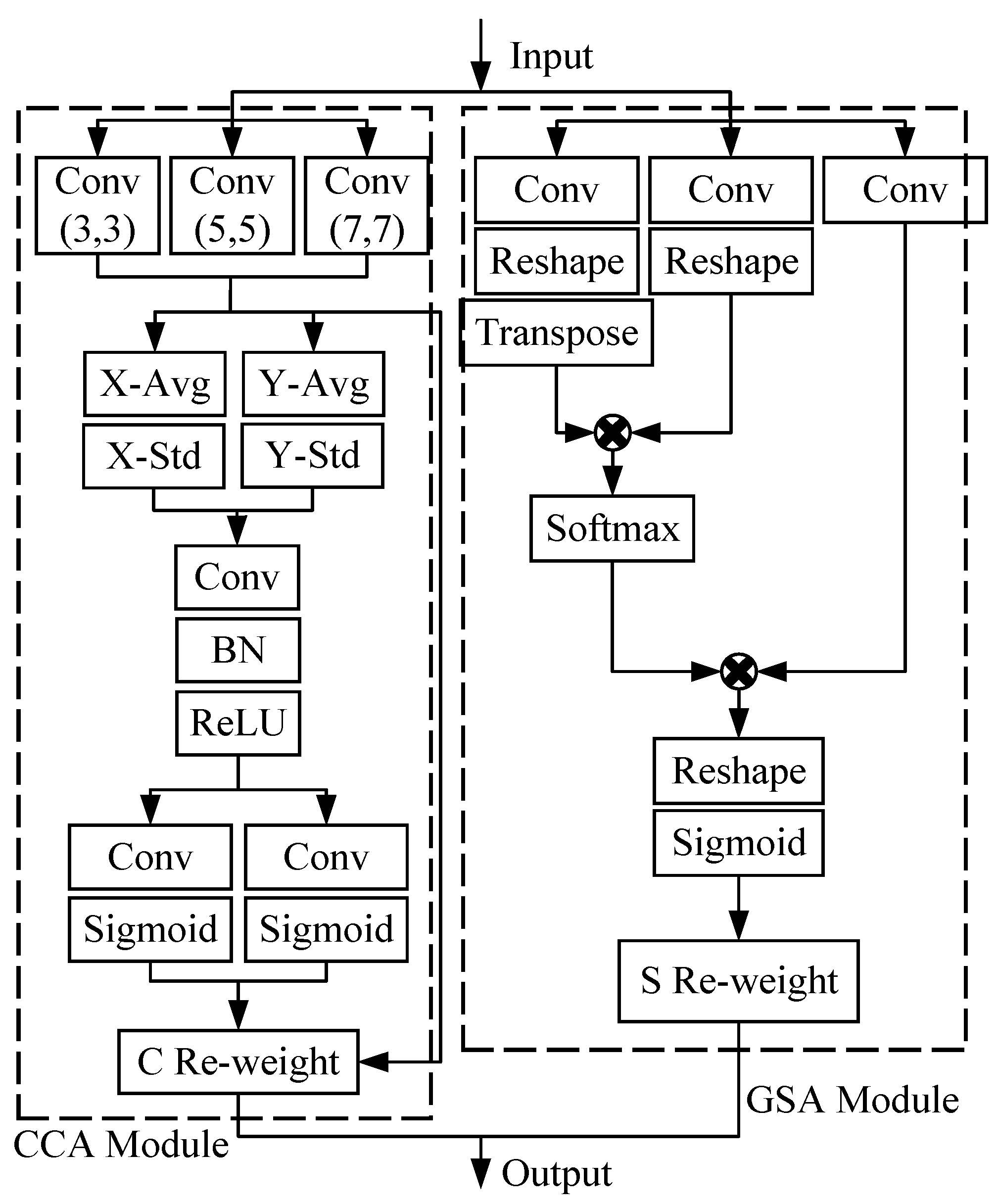
Recently, various attention modules have been proposed to capture channel and spatial information of high-dimension data, such as CBAM [36], DANet [37], and EPSANet [38]. As shown in Figure 5, we propose a multi-attention module called CMAN, which consists of a pyramid coordinate channel attention (CCA) module and a global spatial attention (GSA) module. It extrapolates the attentional maps along the spectral channels and global spatial dimensions, and then multiplies the attentional maps with the input for adaptive feature optimization to obtain deep spatial and spectral features of the input data.

4.3.1. Coordinate Channel Attention Module

In this research, we propose the CCA mechanism to acquire spectral channel weights embedded with positional information. A pyramid structure is adopted to extract feature information of different sizes and increase the pixel-level receptive field. In order to alleviate the positional information loss, we factorize channel attention into two parallel feature encoding strings which acquire average pooling and standard deviation pooling in the H (horizontal) coordinate and V (vertical) coordinate separately. The CCA module can effectively integrate spatial coordinate information into the generated attention maps. Given an arbitrary input $\mathbf{U}\in {\mathbb{R}}^{H\times W\times C}$ for each channel, H and W are the spatial dimensions, C is the channel dimension. The conventional average pooling and standard deviation pooling steps can be formulated as follows,

$$z_{c1}=\frac{1}{H\times W}\sum _{i=1}^H\sum _{j=1}^{W}u(i,j,v)$$

(22)

$$z_{c2}=\sqrt{\frac{1}{H\times W}\sum _{i=1}^H\sum _{j=1}^W{\left(u\right(i,j,v)-\mu )}^2}.$$

(23)

In the proposed attention module, we use two spatial extents of pooling kernels to encode each channel along the horizontal coordinate and the vertical coordinate, respectively. Thus, the average pooling and standard deviation pooling at fixed horizontal position h can be formulated as,

$$z_{c1}\left(h\right)=\frac{1}{W}\sum _{0\le jW}u(h,j,v)$$

(24)

$$z_{c2}\left(h\right)=\sqrt{\frac{1}{W}\sum _{0\le jW}{\left(u\right(h,j,v)-\mu )}^2}$$

(25)

Similarly, the average pooling and standard deviation pooling at given vertical position w can be written as,

$$z_{c1}\left(w\right)=\frac{1}{H}\sum _{0\le iH}u(i,w,v)$$

(26)

$$z_{c2}\left(w\right)=\sqrt{\frac{1}{H}\sum _{0\le iH}{\left(u\right(i,w,v)-\mu )}^2}.$$

(27)

The two strings can capture long-range dependencies along one spatial direction and preserve precise positional information along the other spatial direction. This allows the module to aggregate features along the two spatial directions, respectively, and generate a pair of direction-aware feature maps.

Given the aggregated feature maps, we concatenate them and then send them to a shared convolutional transformation function F,

$$\Gamma =\delta \left(F\left([z^h,z^w]\right)\right)$$

(28)

where [] denotes the concatenation operation along the spatial dimension, $\delta$ is a non-linear activation function. Then, $\Gamma$ is divided into two distinct parameters along the spatial dimension. Another two convolutional transformations $F_h(·)$ and $F_w(·)$ are utilized to separately transform ${\Gamma }^h$ and ${\Gamma }^w$ to parameters with the same channel number to the input $\mathbf{U}$,

$$g_c^h=\sigma \left(F_h\left({\Gamma }^h\right)\right),g_c^w=\sigma \left(F_w\left({\Gamma }^w\right)\right)$$

(29)

where, $\sigma$ is the sigmoid function. Then, the output of each channel can be written as,

$$y_c(i,j)=x_c(i,j)\times g_c^h\left(i\right)\times g_c^w\left(j\right).$$

(30)

4.3.2. Global Spatial Attention Module

We adopt a non-local attention module to model the global spatial context and capture the internal dependency of features. The input feature $\mathbf{U}\in {\mathbb{R}}^{H\times W\times C}$ is convolved to generate two new feature maps $\mathbf{B}$ and $\mathbf{C}$, where $\{\mathbf{B},\mathbf{C}\}\in {\mathbb{R}}^{H\times W\times C}$. Then we reshape $\mathbf{B}$ and $\mathbf{C}$ to ${\mathbf{V}}_1\in {\mathbb{R}}^{N\times C}$ and ${\mathbf{V}}_2\in {\mathbb{R}}^{N\times C}$, where $N=H\times W$ is the number of spatial pixels. The transpose of feature map ${\mathbf{V}}_1$ is multiplicated with the feature map ${\mathbf{V}}_2$, and a softmax layer is applied to calculate the global spatial attention map $\mathbf{T}\in {\mathbb{R}}^{N\times N}$.

$$T(i,j)=\frac{exp\left({\mathbf{V}}_{1i}^{\mathrm{T}}·{\mathbf{V}}_{2j}\right)}{{\displaystyle \sum _{i=1}^N}exp\left({\mathbf{V}}_{1i}^{\mathrm{T}}·{\mathbf{V}}_{2j}\right)}$$

(31)

where ${\mathbf{V}}_{1i}$ is the $i^{th}$ column of ${\mathbf{V}}_1$ and ${\mathbf{V}}_{2i}$ is the $j^{th}$ column of ${\mathbf{V}}_2$.

Meanwhile, we feed the feature $\mathbf{U}$ into a convolution layer to generate a new feature map $\mathbf{D}\in {\mathbb{R}}^{H\times W\times C}$ and reshape it to ${\mathbf{V}}_3\in {\mathbb{R}}^{N\times C}$, then we perform a matrix multiplication between the third feature map $\mathbf{D}$ and the transpose of $\mathbf{T}$ and reshape the result to $\mathbf{S}\in {\mathbb{R}}^{H\times W\times C}$ to obtain the global spatial attention weights.

4.4. Joint Loss Function

We adopt $l_1$ normalization to construct the loss function of the G-net. The G-net included sub-loss function of four generated constraint parts: (1) generation constraint of AENet1 $L_{\mathrm{g}1}={∥{\mathbf{X}}_{\mathrm{s}}-{\widehat{\mathbf{X}}}_{\mathrm{s}}^{\mathrm{a}}∥}_1$, (2) generation constraint of DG block $L_{\mathrm{g}2}={∥{\mathbf{X}}_{\mathrm{s}}-{\widehat{\mathbf{X}}}_{\mathrm{s}}^{\mathrm{b}}∥}_1$, (3) generation constraint of AENet2 $L_{\mathrm{g}3}={∥{\mathbf{X}}_{\mathrm{m}}-{\widehat{\mathbf{X}}}_{\mathrm{m}}∥}_1$, (4) generation constraint of LR-MSI $L_{\mathrm{g}4}={∥{\mathbf{Z}}_1-{\mathbf{Z}}_2∥}_1$. The corresponding loss function is given as follows,

$$L_3={∥{\mathbf{X}}_{\mathrm{s}}-{\widehat{\mathbf{X}}}_{\mathrm{s}}^{\mathrm{a}}∥}_1+{∥{\mathbf{X}}_{\mathrm{s}}-{\widehat{\mathbf{X}}}_{\mathrm{s}}^{\mathrm{b}}∥}_1+{∥{\mathbf{X}}_{\mathrm{m}}-{\widehat{\mathbf{X}}}_{\mathrm{m}}∥}_1+{∥{\mathbf{Z}}_1-{\mathbf{Z}}_2∥}_1.$$

(32)

The sum-to-one of abundances are satisfied by following loss function,

$$L_4={∥\mathbf{1}-\sum _{j=1}^p{\mathbf{A}}_j∥}_1+{∥\mathbf{1}-\sum _{j=1}^p{\mathbf{A}}_{\mathrm{s},j}^{\mathrm{a}}∥}_1+{∥\mathbf{1}-\sum _{j=1}^p{\mathbf{A}}_{\mathrm{s},j}^{\mathrm{b}}∥}_1$$

(33)

where j indicates the $j^{th}$ endmember, and ${\mathbf{A}}_j$ is the $j^{th}$ row of the abundance matrix $\mathbf{A}$.

Based on the spectral mixing model, each pixel of the HSI is composed of a small number of pure spectral bases. Therefore, the abundance matrices should be sparse. To guarantee the sparsity of the abundance, the Kullback-Leibler (KL) divergence is used to ensure that most of the elements in the abundance matrices are close to a small number,

$$L_5=\sum _{i=1}^s\sum _{j=1}^{p}KL[\beta ∥log\left(\frac{\beta }{a_{i,j}}\right)]=\sum _{i=1}^s\sum _{j=1}^p[\beta log\left(\frac{\beta }{a_{i,j}}\right)+(1-\beta )log\frac{1-\beta }{1-a_{i,j}}]$$

(34)

where s is the number of pixels, p is the number of endmembers, $\beta$ is a sparsity parameter (0.001 in our network), and $a_{ij}$ is the element of the abundance. This loss function constrains all the generation abundances mentioned above.

Ultimately, the fusion problem is solved by constructing a deep learning GAN framework which can optimize the following objective function,

$$L^{*}=\arg \underset{\mathcal{G}}{\min }\underset{{\mathcal{D}}_1,{\mathcal{D}}_2}{\max }(L_1+L_2+L_3+L_4+L_5).$$

(35)

5. Experiments and Analysis

To demonstrate the effectiveness and performance of the proposed GAN architecture on HSI-MSI fusion, we perform ablation analysis of the proposed network and compare the method with other fusion methods.

5.1. Implementation Details

5.1.1. Data Sets

The following experiments are conducted on four widely used HSI data sets, Pavia University, Indian Pines, Washington DC, and University of Houston. The Pavia University data were acquired by the ROSIS-3 optical airborne sensor in 2003. This image consists of 610 × 340 pixels with a ground sampling distance (GSD) of 1.3 m and spectral range of 430–840 nm in 115 bands. The University of Houston data were used in the 2018 IEEE GRSS Data Fusion Contest, and consist of 601 × 2384 pixels with a 1 m GSD. The data cover the spectral range 380–1050 nm with 48 bands. The Indian Pines data were acquired by the AVIRIS in 1992. This image consists of 145 × 145 pixels with a 20 m GSD and the spectral range is 400–2500 nm covering 224 bands. The Washington DC data were acquired by the HYDICE sensor in 1995. This image has an area of 1280 × 307 pixels and a GSD of 2.5 m. The spectral range is 400–2500 nm, consisting of 210 bands.

In the experiment, we selected and cropped these hyperspectral datasets, which are adopted as the original HR-HSI data sets. The LR-HSI is synthesized by spatially downsampling the original HSI data sets by using Gaussian filters. For all datasets, the scaling ratio was set to 4. To synthesize the HR-MSI, the SRF characteristics of the Landsat 8 were used. According to the spectral range of the HSI data sets, the blue–green–red bands SRFs of the Landsat 8 were used to synthesize the RGB images of Pavia University and University of Houston data sets. And the blue to SWIR2 part SRFs of the Landsat 8 were used to form 4-band MSIs of Indian Pines and Washington DC data sets.

Table 1. Original HR I Data Sets Used In The Experiments.

Data Sets	Pavia University	Houston University	Indian Pines	Washington D.C.
Spatial size of HSI	336 × 336	320 × 320	144 × 144	304 × 304
Spectral range of HSI	466–834 nm	403–1047 nm	400–2500 nm	400–2500 nm
Number bands of HSI	103	46	191	191
Downsampling ratio	4	4	4	4
SpatialIze of LR HSI	84 × 84	80 × 80	36 × 36	76 × 76
Bands of MSI	Blue-Green-Red	Blue-Green-Red	Blue to SWIR2	Blue to SWIR2

summarizes the parameters of the data sets used in following experiment.

5.1.2. Model Training

The proposed network is implemented under PyTorch framework. The model is trained by using an Adam optimizer with the default parameters ${\beta }_1=0.9$, ${\beta }_2=0.999$, and $\epsilon ={10}^{-8}$. The learning rate is initialized with $5\times {10}^{-4}$, which applied a linear decay drop-step schedule to adjust the learning rate during training. The batch size is set to 1. And the input images can be randomly cropped to form mini-batch and sent to the model training in turn.

5.1.3. Performance Metrics

Six different objective metrics are adopted to compare the fusion results $\widehat{\mathbf{Y}}$ and the ground truth $\mathbf{Y}$. They are the root mean square error (RMSE), mean relative absolute error (MRAE), peak signa noise ratio (PSNR), average structural similarity (aSSIM), spectral angle mapper (SAM), and erreur relative globale adimensionnelle de synthèse (ERGAS). The RMSE is defined as,

$$RMSE(\mathbf{Y},\widehat{\mathbf{Y}})=\sqrt{\frac{1}{KN}\sum _j^K\sum _i^N{\left({\mathbf{Y}}_i^j-{\widehat{\mathbf{Y}}}_i^j\right)}^2}$$

(36)

where j is the jth band, I is the spatial location of pixels, K is the number of bands, and N is the number of spatial pixels.

The MRAE is given as,

$$MRAE(\mathbf{Y},\widehat{\mathbf{Y}})=\frac{{\sum }_{i,j}\frac{\left|{\mathbf{Y}}_i^j-{\widehat{\mathbf{Y}}}_i^j\right|}{{\widehat{\mathbf{Y}}}_i^j}}{\left|\widehat{\mathbf{Y}}\right|}.$$

(37)

The PSNR is given as,

$$PSNR(\mathbf{Y},\widehat{\mathbf{Y}})=20{log}_{10}\frac{1}{RMSE}.$$

(38)

For HSI data, we employ the average of channel-wised SSIMs to quantitatively evaluate the spatial consistency, and it is given as,

$$aSSIM(\mathbf{Y},\widehat{\mathbf{Y}})=\frac{1}{K}\sum _j^K{\left(\frac{(2\overline{{\mathbf{Y}}^j}\overline{{\widehat{\mathbf{Y}}}^j}+C_1)(2{\sigma }_{{\mathbf{Y}}^j,{\widehat{\mathbf{Y}}}^j}+C_2)}{({\overline{{\mathbf{Y}}^j}}^2+{\overline{{\widehat{\mathbf{Y}}}^j}}^2+C_1)({\sigma }_{{\mathbf{Y}}^j}^2+{\sigma }_{{\widehat{\mathbf{Y}}}^j}^2+C_2)}\right)}_j$$

(39)

where $C_1$ and $C_2$ are constants, ${\sigma }_{\mathbf{Y}}$ and ${\sigma }_{\widehat{\mathbf{Y}}}$ are the standard deviations of images $\mathbf{Y}$ and $\widehat{\mathbf{Y}}$, and ${\sigma }_{\mathbf{Y},\widehat{\mathbf{Y}}}$ is the covariance.

The spectral angle distance (SAD) is used to describe the similarity between a restored spectrum and the ideal spectrum of a single pixel, and it is given as,

$$SAD({\mathbf{Y}}_i,{\widehat{\mathbf{Y}}}_i)=\frac{180}{\pi }arccos\frac{{\mathbf{Y}}_i·{\widehat{\mathbf{Y}}}_i}{∥{\mathbf{Y}}_i∥·∥{\widehat{\mathbf{Y}}}_i∥}.$$

(40)

The SAM is the average value of the SADs of all the pixels in the scene, and it can be given as following,

$$SAM(\mathbf{Y},\widehat{\mathbf{Y}})=\frac{1}{N}\sum _i^{N}SAD({\mathbf{Y}}_i,{\widehat{\mathbf{Y}}}_i).$$

(41)

The ERGAS is given as,

$$ERGAS=100\frac{h}{l}\sqrt{\frac{1}{K}{\sum _j^K\left[RMSE\left({\widehat{\mathbf{Y}}}^j\right)/Mean\left({\widehat{\mathbf{Y}}}^j\right)\right]}^2}$$

(42)

where h/l is the ratio of high resolution to low resolution.

5.2. Ablation Experiments

To examine the necessity of various aspects of the method, multiple ablation studies on the proposed technique were conducted.

5.2.1. Generation Constraints

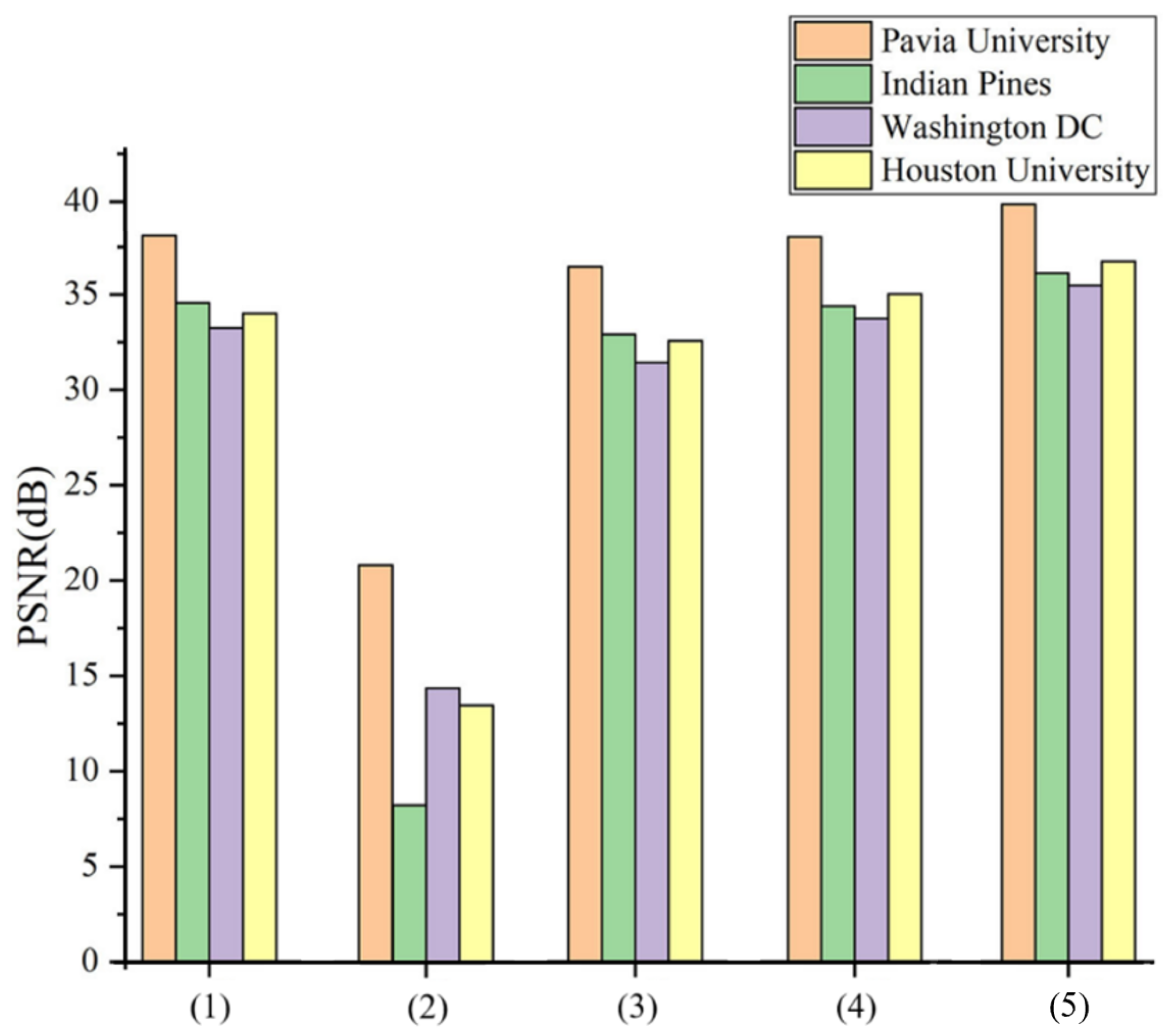
As described in Section 4.4, the definition of loss function $L_3$ is closely correlated with the four data reconstruction modules of the G-net. In this section, we remove one sub-loss function at a time to demonstrate the effectiveness of the corresponding module.

Case 1: removing generation constraint of AENet1 $L_{\mathrm{g}1}$, and the loss function is given as,

$$L_{3-1}={∥{\mathbf{X}}_{\mathrm{s}}-{\widehat{\mathbf{X}}}_{\mathrm{s}}^{\mathrm{b}}∥}_1+{∥{\mathbf{X}}_{\mathrm{m}}-{\widehat{\mathbf{X}}}_{\mathrm{m}}∥}_1+{∥{\mathbf{Z}}_1-{\mathbf{Z}}_2∥}_1$$

(43)

Case 2: removing generation constraint of DG block $L_{\mathrm{g}2}$, and the loss function is rewritten as,

$$L_{3-2}={∥{\mathbf{X}}_{\mathrm{s}}-{\widehat{\mathbf{X}}}_{\mathrm{s}}^{\mathrm{a}}∥}_1+{∥{\mathbf{X}}_{\mathrm{m}}-{\widehat{\mathbf{X}}}_{\mathrm{m}}∥}_1+{∥{\mathbf{Z}}_1-{\mathbf{Z}}_2∥}_1$$

(44)

Case 3: removing generation constraint of AENet2 $L_{\mathrm{g}3}$, and the loss function is given as,

$$L_{3-3}={∥{\mathbf{X}}_{\mathrm{s}}-{\widehat{\mathbf{X}}}_{\mathrm{s}}^{\mathrm{a}}∥}_1+{∥{\mathbf{X}}_{\mathrm{s}}-{\widehat{\mathbf{X}}}_{\mathrm{s}}^{\mathrm{b}}∥}_1+{∥{\mathbf{Z}}_1-{\mathbf{Z}}_2∥}_1$$

(45)

Case 4: removing generation constraint of LR-MSI $L_{\mathrm{g}4}$, and the loss function is rewritten as,

$$L_{3-4}={∥{\mathbf{X}}_{\mathrm{s}}-{\widehat{\mathbf{X}}}_{\mathrm{s}}^{\mathrm{a}}∥}_1+{∥{\mathbf{X}}_{\mathrm{s}}-{\widehat{\mathbf{X}}}_{\mathrm{s}}^{\mathrm{b}}∥}_1+{∥{\mathbf{X}}_{\mathrm{m}}-{\widehat{\mathbf{X}}}_{\mathrm{m}}∥}_1$$

(46)

Case 5: using the complete generation constraint of G-net with loss function given by Equation (32).

The results of all the cases on all four datasets are illustrated in Figure 6. It can be seen that the performance drops as one constraint is removed. Furthermore, in case 2, the removal of the DG block causes drastically performance drop. This indicates the branch of DG strongly affects the overall fusion performance. Moreover, case 4 also shows the advantage of the learnable spatial and spectral degradation module in improving the fusion result.

5.2.2. Attention Mechanism

To investigate the effectiveness of the proposed multi-attention module CMAN, ablation analysis was conducted by removing CMAN module and replacing CMAN with other attention mechanisms. Three multi-attention mechanisms included are the following,

(1) CBAM [38]: A multi-attention module combines both channel and spatial attention mechanisms.

(2) DANet [39]: A multi-attention module introduces self-attention mechanism in both channel and spatial attention mechanism.

(3) EPSANet [40]: An attention module adopts a pyramid structure to extract multi-scale spatial information effectively.

In this section, we choose one RGB data set (Pavia University) and one MSI data set (Indian Pines) to demonstrate the comparisons on RGB-HSI and MSI-HSI fusion, respectively.

Table 2. Comparisons of different attention modules (Pavia University).

	SAM (°)	PSNR (dB)	aSSIM
No-Attention	3.4976	37.2953	0.9025
Attention-CBAM	3.9612	36.7323	0.8987
Attention-DANet	3.4474	38.0712	0.9065
Attention-EPSANet	3.4739	37.6053	0.9052
Attention-CMAN	3.4002	38.9132	0.9140

and

Table 3. Comparisons of different attention modules (Indian Pines).

	SAM (°)	PSNR (dB)	aSSIM
No-Attention	2.3201	32.7298	0.9177
Attention-CBAM	2.3947	32.1214	0.9133
Attention-DANet	2.2839	33.6114	0.9208
Attention-EPSANet	2.2926	33.0981	0.9190
Attention-CMAN	2.2447	34.3232	0.9561

summarize the quantitative results of Pavia University and Indian Pines datasets with/without attention mechanisms. It is obvious that the proposed CMAN performs better than the other attention modules. The results of the CBAM module are even worse than that of the non-attention network. This means that not all attention mechanisms are suitable for the proposed GAN fusion framework.

5.2.3. Nonnegative Constraint Function

In order to enforce the nonnegative constraints of abundance $\mathbf{A}$, a nonnegative constraint function is applied to the output of the last convolution layer of both the encoder nets. In addition, the weights of the convolution layer containing the endmember $\mathbf{E}$, the spatial degradation layer, and the spectral degradation layer should also meet the nonnegative constraints. Since the weights of these layers may be updated to a negative value after the backpropagation, nonnegative constraint functions are also applied to these layers after the weights are updated. Both the softmax function and the clamp function can restrict the property of the nonnegative.

The clamp function used in the proposed model is set as,

$$clamp\left(a_{ij}\right)\left\{\begin{array}{cc}0& a_{ij}\le 0\\ a_{ij}& 0\le a_{ij}\le 1\\ 1& a_{ij}\ge 1\end{array}\right.$$

(47)

where $a_{ij}$ is the element of the abundance coefficient. In contrast, the gradient of the clamp function is updated faster in the range [0, 1].

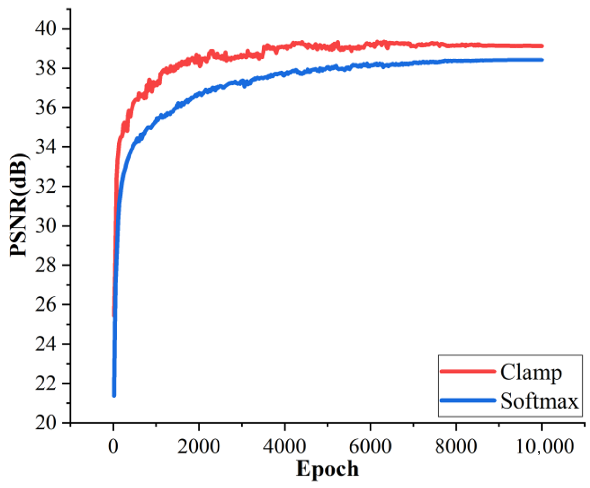
The two functions are tested in the network separately. The convergence behavior over the training epochs is shown in Figure 7.

It can be observed that the clamp function leads to a better reconstruction accuracy with lower training epochs than the softmax function does. Therefore, the clamp function is adopted in the proposed network.

5.2.4. Ablation Study of GAN

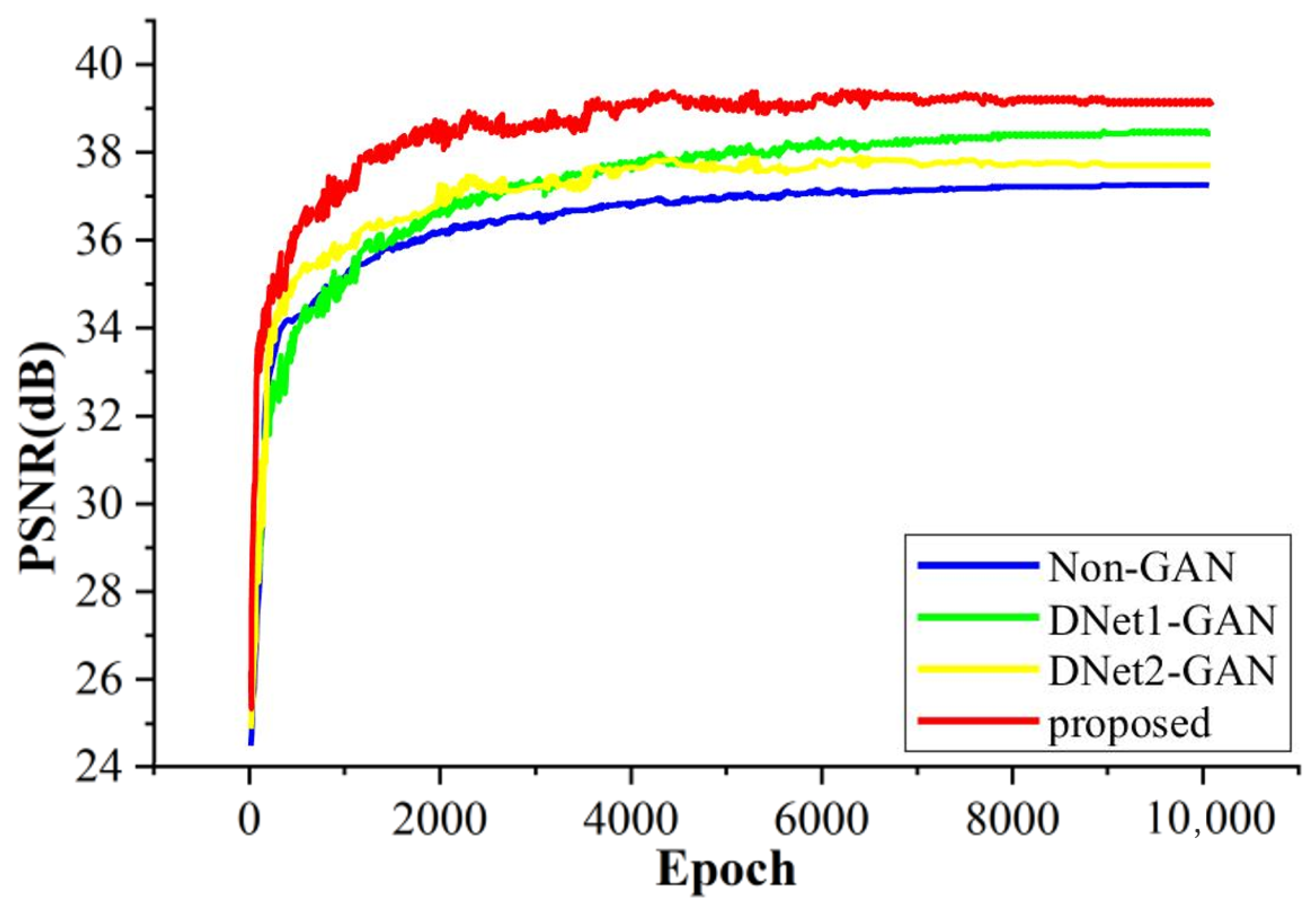
The discriminators of GAN are designed to make the output of the autoencoder closer to the input in feature and semantic information. In order to show the effectiveness of the adversarial training of the GAN framework, the discriminator networks with corresponding loss functions $L_1$ and $L_2$ are removed to acquire a Non-GAN network for HSI-MSI fusion. Meanwhile, we also test the GAN framework with either D-Net1 or D-Net2, respectively. Figure 8 shows the convergence behaviors without/with different discriminator nets over the Pavia University data set. The results demonstrate that the GAN frameworks outperform the Non-GAN network.

In addition, we chose the Pavia University data set and the Indian Pines data set to compare the performance of GAN architecture on RGB-HSI and MSI-HSI fusion, respectively. As shown in

Table 4. Ablation experiments on adversarial network.

Dataset		SAM (°)	PSNR (dB)	aSSIM
Pavia University	Non-GAN	3.6494	36.8070	0.8996
	DNet1-GAN	3.4685	38.3198	0.9119
	DNet2-GAN	3.5760	37.2763	0.9036
	proposed GAN	3.4002	38.9132	0.9140
Indian Pines	Non-GAN	2.3519	32.5224	0.9174
	DNet1-GAN	2.2833	33.8712	0.9394
	DNet2-GAN	2.3118	32.9576	0.9245
	proposed GAN	2.2447	34.3232	0.9561

, the proposed GAN can achieve much better fusion results in all metrics.

5.3. Comparison Experiments

In this section, we make comprehensive comparisons to verify the reliability and validity of the proposed method. Four state-of-the-art deep-learning HSI-MSI fusion methods used for comparison are the following:

(1) CUCA [35] consists of a two-stream convolutional autoencoder with a cross-attention module.

(2) HYCO [33] is composed of three coupled autoencoder networks.

(3) UMAG [32] is an unsupervised multi-attention-guided network.

(4) PGAN [31] is a physical-based GAN with a multiscale channel attention and a spatial attention fusion module.

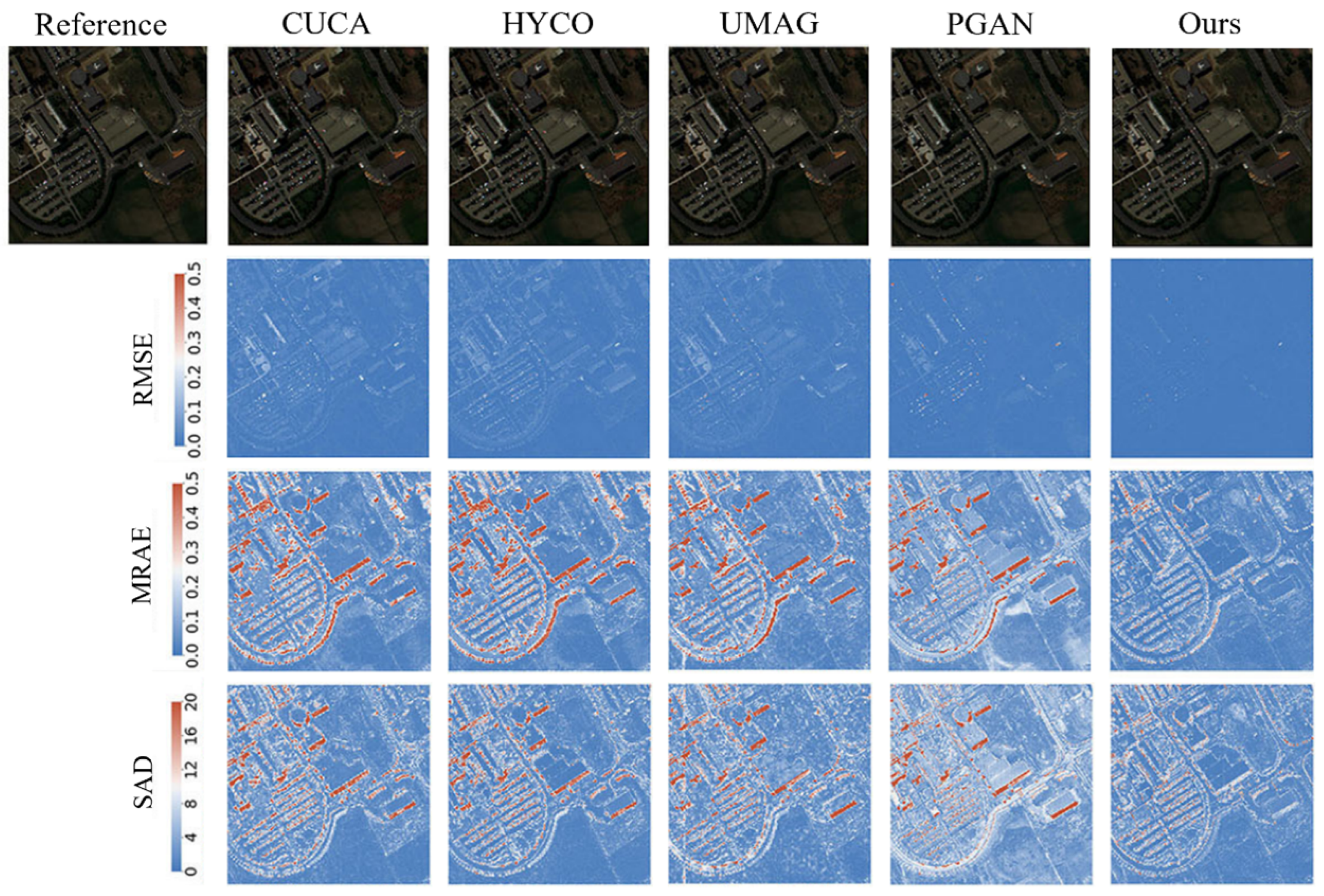
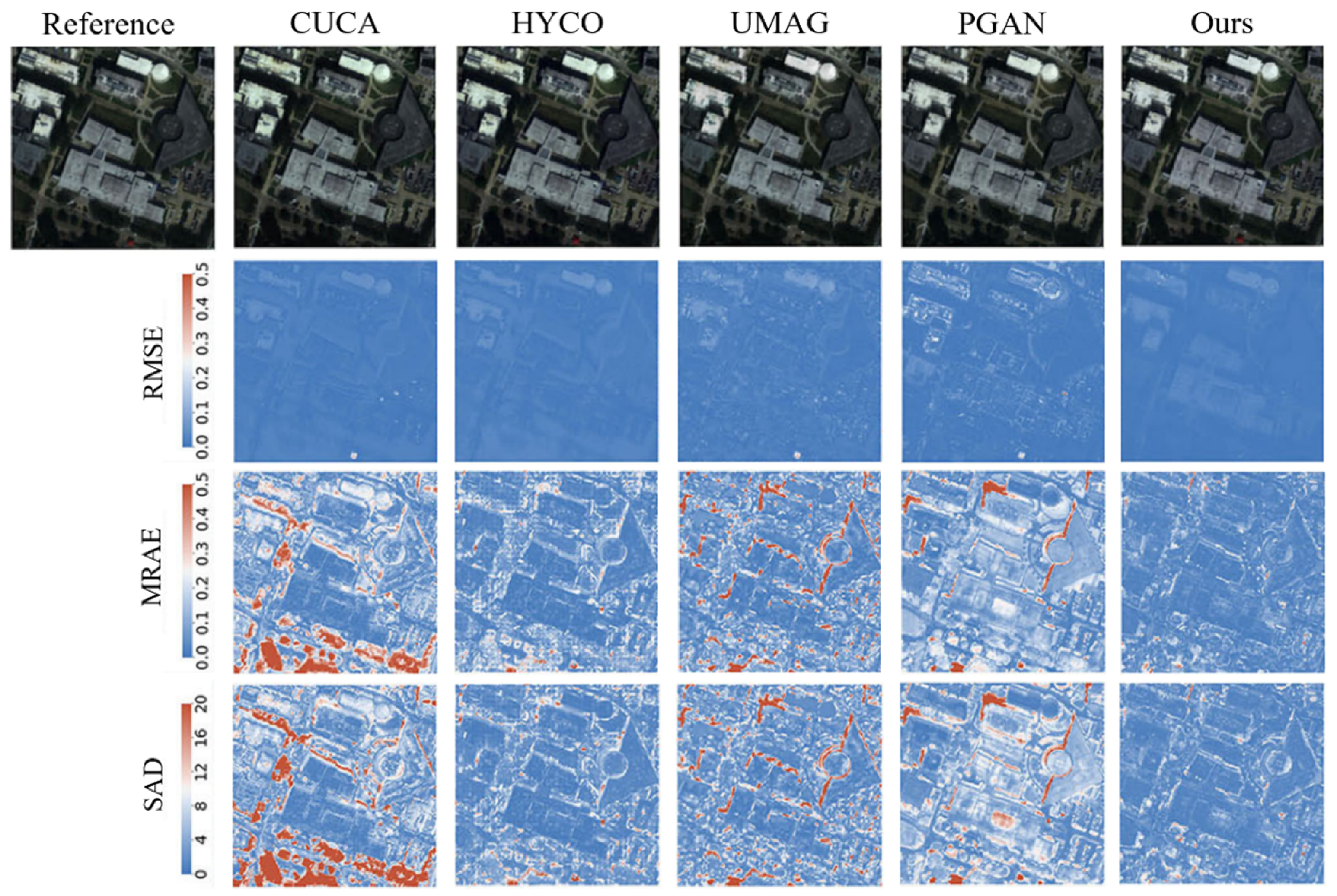
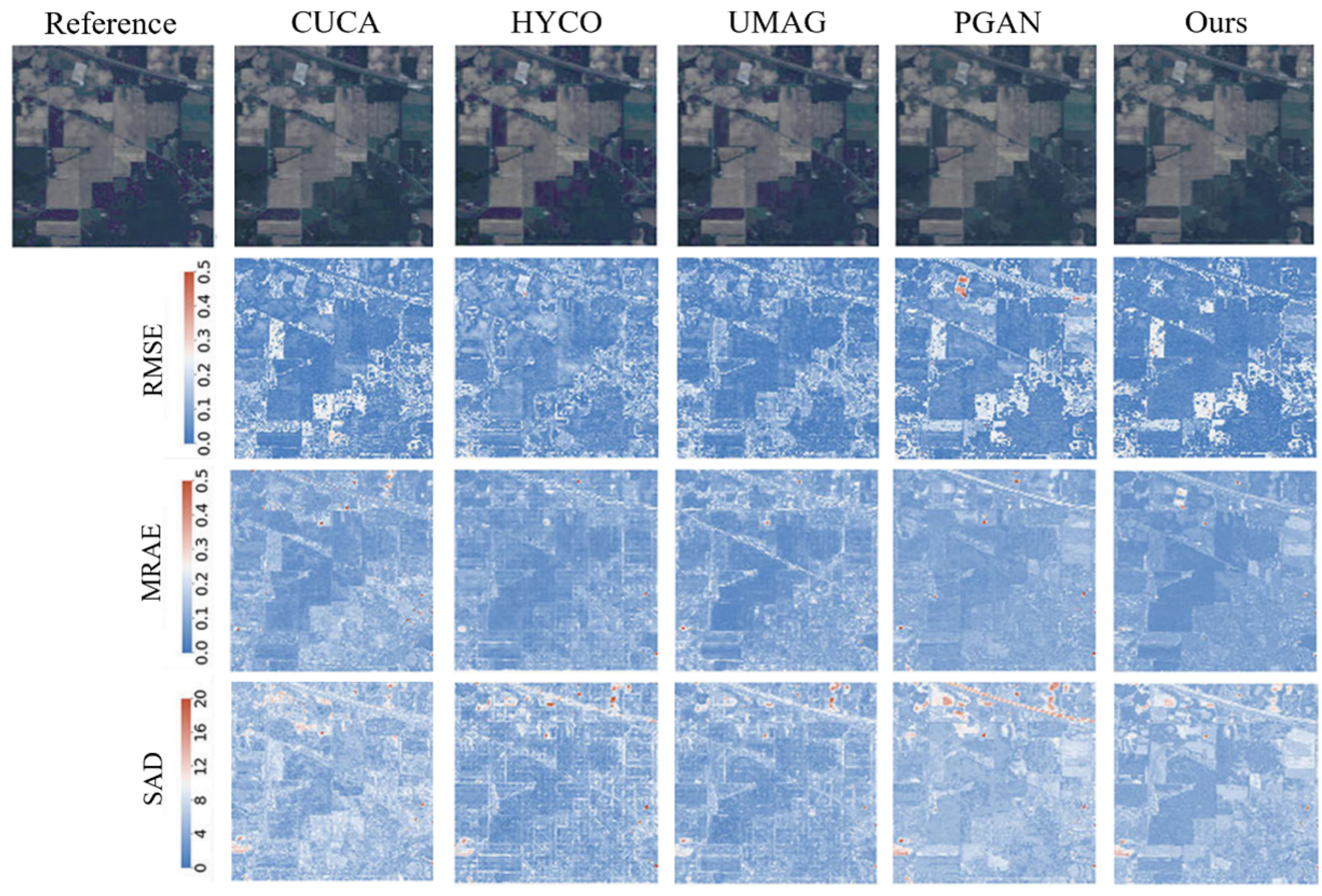
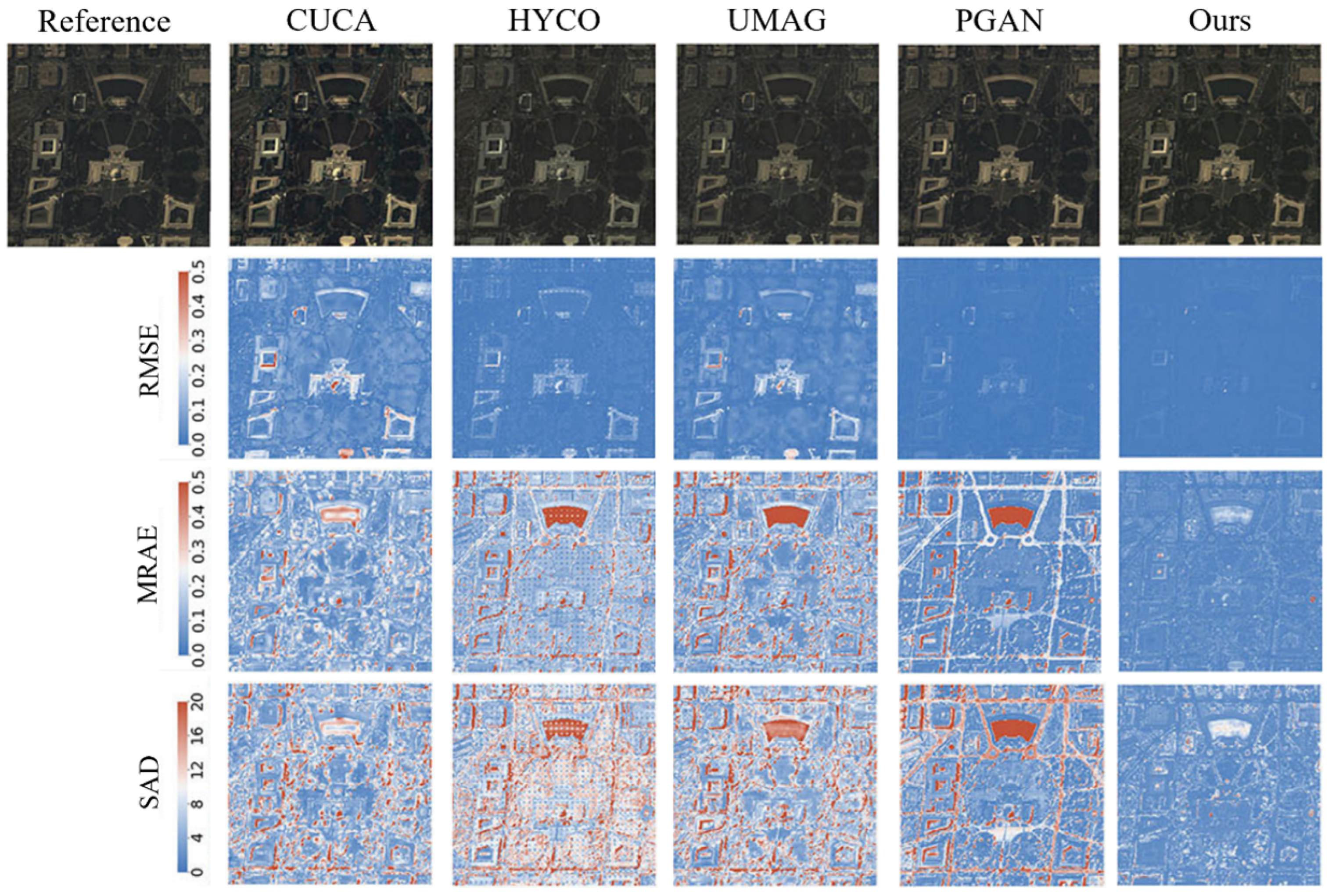
Since it is hard to visually discern the differences among false-color images of fused results, we use heatmaps of RMSE, MRAE and SAD to visually demonstrate the performance of the fusion methods. The RMSE heatmap and the MRAE heatmap can be considered to show the pixelwise error for the reconstructed image cube. The SAD heatmap represents the spectral consistency of each pixel in the fused HSI. We also use PSNR, aSSIM, SAM and ERGAS to quantitatively compare these methods. The PSNR and aSSIM are the measures of the spatial quality. The SAM is used to evaluate overall spectral consistency of the reconstructed HSI. And the ERGAS is a global statistical measure used to evaluate the dimensionless global error for fused data.

5.3.1. Pavia University

We first conducted HSI-RGB fusion on the Pavia University and Houston University datasets. The visual representation of the performance of each fusion method on the Pavia University dataset is shown in Figure 9. From the visual perspective, the proposed method generates results with much less spatial errors and spectral distortions than the other four methods. Among the other four methods, PGAN is visually better on RMSE heatmap, but worse on MRAE and SAD heatmaps. According to the quantitative metrics summarized in

Table 5. Objective evaluation metrics on Pavia University dataset.

	SAM (°)	PSNR (dB)	aSSIM	ERGAS
CUCA	3.4810	37.5222	0.9047	2.7435
HYCO	3.5015	36.9652	0.9002	2.8068
UMAG	4.0694	36.2267	0.8973	2.8824
PGAN	5.3427	33.1369	0.8623	4.0075
Proposed	3.4002	38.9132	0.9140	2.6955

, the proposed method produces the best results in all the indicators. PGAN performs worse than the other methods do. Meanwhile, CUCA performs second best on the Pavia University dataset.

5.3.2. Houston University

The comparison on Houston University dataset is shown in Figure 10 and

Table 6. Objective evaluation metrics on Houston University dataset.

	SAM (°)	PSNR (dB)	aSSIM	ERGAS
CUCA	7.9230	28.9063	0.8306	2.9949
HYCO	3.2576	34.0117	0.9170	1.3078
UMAG	4.7106	31.8105	0.8974	1.4552
PGAN	4.9899	29.0370	0.8612	2.0462
Proposed	2.6670	35.1123	0.9457	1.0252

, and our proposed method achieves the best results. HYCO performs second best on both visual perspective and quantitative indicators. And CUCA performs worst on Washington DC dataset.

5.3.3. Indian Pines

Then we conducted HSI-MSI fusion on Indian Pines and Washington DC datasets. On Indian Pines dataset, Figure 11 shows that CUCA, HYCO, UMAG and the proposed method are similar in terms of visual effects. In terms of quantitative indicators given in

Table 7. Objective evaluation metrics on Indian Pines dataset.

	SAM (°)	PSNR (dB)	aSSIM	ERGAS
CUCA	2.3812	32.0225	0.9125	1.5949
HYCO	2.2692	33.8168	0.9393	1.2740
UMAG	2.2854	33.6857	0.9217	1.3392
PGAN	2.9288	31.1590	0.8963	1.6710
Proposed	2.2447	34.3232	0.9561	1.1946

, our method is superior to the other four methods, and HYCO is slightly better than the other three methods. It is obvious that the differences among fusion results are small. The reason may be that the distribution of ground objects in Indian Pines dataset is relatively simple.

5.3.4. Washington DC

Figure 12 shows the comparison on the Washington DC dataset. From the perspective of visual performance, the performance of the four comparison algorithms on this dataset is relatively poor. The quantitative indicators are summarized in

Table 8. Objective evaluation metrics on Washington DC dataset.

	SAM (°)	PSNR (dB)	aSSIM	ERGAS
CUCA	5.8450	30.0319	0.8972	1.7830
HYCO	7.7087	28.7836	0.8315	2.3315
UMAG	8.0205	29.9389	0.8461	2.2540
PGAN	7.5995	31.1618	0.8619	2.1821
Proposed	3.2828	33.9646	0.9215	1.3959

. Our method is significantly better than the other four methods in both visual effects and evaluation metrics. PGAN is visually second best on RMSE heatmap and PSNR indicator, while CUCA performs second best on the rest quantitative indicator.

In conclusion, the proposed method achieves best performance on all four datasets when compared with the other four methods. The other methods may perform well on a specific dataset, but fail on the other datasets. This also demonstrates the consistent superiority of the proposed methods.

6. Conclusions

In this article, we proposed a novel unsupervised GAN to address the HSI and MSI fusion problem with arbitrary PSFs and SRFs. This GAN consists of one generator network and two discriminator networks which employ the spatial and spectral degradation models. In order to extract spectral information from the LR HSI and spatial–contextual information from the MSI, the generator network employs two streams of autoencoders. In parallel, we use DG Block to reconstruct another HSI to do subsequent discrimination. Through the attention module CMAN designed in encoder nets, we also allocate the weight of feature importance. The discriminator nets extract multi-dimensional features of the input and output from generator networks to evaluate the authenticity. Using the joint loss function, the proposed method provides a simple and straightforward end-to-end training approach. Four open datasets were used for the comparison experiments, which demonstrate that the proposed method performs better overall.

References

1. Gao, L.; Li, J.; Khodadadzadeh, M.; Plaza, A.; Zhang, B.; He, Z.; Yan, H. Subspace-based support vector machines for hyperspectral image classification. IEEE Geosci. Remote Sens. Lett. 2014, 12, 349–353. [Google Scholar]
2. Hong, D.; Wu, X.; Ghamisi, P.; Chanussot, J.; Yokoya, N.; Zhu, X.X. Invariant attribute profiles: A spatial-frequency joint feature extractor for hyperspectral image classification. IEEE Trans. Geosci. Remote Sens. 2020, 58, 3791–3808. [Google Scholar] [CrossRef]
3. Cao, X.; Yao, J.; Xu, Z.; Meng, D. Hyperspectral image classification with convolutional neural network and active learning. IEEE Trans. Geosci. Remote Sens. 2020, 58, 4604–4616. [Google Scholar] [CrossRef]
4. Cao, X.; Yao, J.; Fu, X.; Bi, H.; Hong, D. An enhanced 3-D discrete wavelet transform for hyperspectral image classification. IEEE Geosci. Remote Sens. Lett. 2020, 18, 1104–1108. [Google Scholar] [CrossRef]
5. Guo, Q.; Zhang, B.; Ran, Q.; Gao, L.; Li, J.; Plaza, A. Weighted-RXD and linear filter-based RXD: Improving background statistics estimation for anomaly detection in hyperspectral imagery. IEEE J. Sel. Top. Appl. Earth Obs. Remote Sens. 2014, 7, 2351–2366. [Google Scholar] [CrossRef]
6. Li, C.; Gao, L.; Wu, Y.; Zhang, B.; Plaza, J.; Plaza, A. A real-time unsupervised background extraction-based target detection method for hyperspectral imagery. J. Real-Time Image Process. 2018, 15, 597–615. [Google Scholar] [CrossRef]
7. Wu, X.; Hong, D.; Tian, J.; Chanussot, J.; Li, W.; Tao, R. ORSIm detector: A novel object detection framework in optical remote sensing imagery using spatial-frequency channel features. IEEE Trans. Geosci. Remote Sens. 2019, 57, 5146–5158. [Google Scholar] [CrossRef]
8. Wu, X.; Hong, D.; Chanussot, J.; Xu, Y.; Tao, R.; Wang, Y. Fourier-based rotation-invariant feature boosting: An efficient framework for geospatial object detection. IEEE Geosci. Remote Sens. Lett. 2019, 17, 302–306. [Google Scholar] [CrossRef]
9. He, W.; Zhang, H.; Zhang, L.; Philips, W.; Liao, W. Weighted sparse graph based dimensionality reduction for hyperspectral images. IEEE Geosci. Remote Sens. Lett. 2016, 13, 686–690. [Google Scholar] [CrossRef]
10. Hong, D.; Yokoya, N.; Zhu, X.X. Learning a robust local manifold representation for hyperspectral dimensionality reduction. IEEE J. Sel. Top. Appl. Earth Obs. Remote Sens. 2017, 10, 2960–2975. [Google Scholar] [CrossRef]
11. Xu, H.; Zhang, H.; He, W.; Zhang, L. Superpixel-based spatial-spectral dimension reduction for hyperspectral imagery classification. Neurocomputing 2019, 360, 138–150. [Google Scholar] [CrossRef]
12. Hong, D.; Yokoya, N.; Chanussot, J.; Xu, J.; Zhu, X.X. Learning to propagate labels on graphs: An iterative multitask regression framework for semi-supervised hyperspectral dimensionality reduction. Isprs J. Photogramm. Remote Sens. 2019, 158, 35–49. [Google Scholar] [CrossRef]
13. Tang, M.; Gao, L.; Marinoni, A.; Gamba, P.; Zhang, B. Integrating spatial information in the normalized P-linear algorithm for nonlinear hyperspectral unmixing. IEEE J. Sel. Top. Appl. Earth Obs. Remote Sens. 2017, 11, 1179–1190. [Google Scholar] [CrossRef]
14. Hong, D.; Zhu, X.X. SULoRA: Subspace unmixing with low-rank attribute embedding for hyperspectral data analysis. IEEE J. Sel. Top. Signal Process. 2018, 12, 135–1363. [Google Scholar] [CrossRef]
15. Yao, J.; Meng, D.; Zhao, Q.; Cao, W.; Xu, Z. Nonconvex-sparsity and nonlocal-smoothness-based blind hyperspectral unmixings. IEEE Trans. Image Process. 2019, 28, 2991–3006. [Google Scholar] [CrossRef]
16. Gomez, R.B.; Jazaeri, A.; Kafatos, M. Wavelet-based hyperspectral and multispectral image fusion. In Proceedings of the Geo-Spatial Image and Data Exploitation II, Orlando, FL, USA, 16–20 April 2001; pp. 36–42. [Google Scholar]
17. Zhang, Y.; He, M. Multi-spectral and hyperspectral image fusion using 3-D wavelet transform. J. Electron. 2007, 24, 218–224. [Google Scholar] [CrossRef]
18. Chen, Z.; Pu, H.; Wang, B.; Jiang, G.-M. Fusion of hyperspectral and multispectral images: A novel framework based on generalization of pan-sharpening methods. IEEE Geosci. Remote Sens. Lett. 2014, 11, 1418–1422. [Google Scholar] [CrossRef]
19. Aiazzi, B.; Baronti, S.; Selva, M. Improving component substitution pansharpening through multivariate regression of MS + Pan data. IEEE Trans. Geosci. Remote Sens. 2007, 45, 3230–3239. [Google Scholar] [CrossRef]
20. Eismann, M.T.; Hardie, R.C. Hyperspectral resolution enhancement using high-resolution multispectral imagery with arbitrary response functions. IEEE Trans. Geosci. Remote Sens. 2005, 43, 455–465. [Google Scholar] [CrossRef]
21. Wei, Q.; Bioucas-Dias, J.; Dobigeon, N.; Tourneret, J.-Y. Hyperspectral and multispectral image fusion based on a sparse representation. IEEE Trans. Geosci. Remote Sens. 2015, 53, 3658–3668. [Google Scholar] [CrossRef]
22. Simoes, M.; Bioucas-Dias, J.; Almeida, L.B.; Chanussot, J. A convex formulation for hyperspectral image superresolution via subspace-based regularization. IEEE Trans. Geosci. Remote Sens. 2014, 53, 3373–3388. [Google Scholar] [CrossRef] [Green Version]
23. Akhtar, N.; Shafait, F.; Mian, A. Bayesian sparse representation for hyperspectral image super resolution. In Proceedings of the IEEE Conference on Computer Vision and Pattern Recognition, Boston, MA, USA, 7–12 June 2015; pp. 3631–3640. [Google Scholar]
24. Kawakami, R.; Matsushita, Y.; Wright, J.; Ben-Ezra, M.; Tai, Y.-W.; Ikeuchi, K. High-resolution hyperspectral imaging via matrix factorization. In Proceedings of the IEEE Conference on Computer Vision and Pattern Recognition, Colorado Springs, CO, USA, 20–25 June 2011; pp. 2329–2336. [Google Scholar]
25. Yokoya, N.; Yairi, T.; Iwasaki, A. Coupled nonnegative matrix factorization unmixing for hyperspectral and multispectral data fusion. IEEE Trans. Geosci. Remote Sens. 2011, 50, 528–537. [Google Scholar] [CrossRef]
26. Lanaras, C.; Baltsavias, E.; Schindler, K. Hyperspectral super-resolution by coupled spectral unmixing. In Proceedings of the IEEE Conference on Computer Vision and Pattern Recognition, Boston, MA, USA, 7–12 June 2015; pp. 3586–3594. [Google Scholar]
27. Dian, R.; Fang, L.; Li, S. Hyperspectral image super-resolution via non-local sparse tensor factorization. In Proceedings of the IEEE Conference on Computer Vision and Pattern Recognition, Honolulu, HI, USA, 18–23 June 2018; pp. 5344–5353. [Google Scholar]
28. Dian, R.; Li, S.; Guo, A.; Fang, L. Deep hyperspectral image sharpening. IEEE Trans. Neural Netw. Learn. Syst. 2018, 29, 5345–5355. [Google Scholar] [CrossRef] [PubMed]
29. Han, X.H.; Shi, B.; Zheng, Y.Q. SSF-CNN:Spatial and Spectral Fusion with CNN for Hyperspectral Image Super-Resolution. In Proceedings of the 2018 25th IEEE International Conference on Image Processing(ICIP), Athens, Greece, 7–10 October 2018; pp. 2506–2510. [Google Scholar]
30. Yang, Q.; Xu, Y.; Wu, Z.; Wei, Z. Hyperspectral and multispectral image fusion based on deep attention network. In Proceedings of the 2019 10th Workshop on Hyperspectral Imaging and Signal Processing: Evolution in Remote Sensing (WHISPERS), Amsterdam, The Netherlands, 24–26 September 2019; pp. 1–5. [Google Scholar]
31. Xiao, J.; Li, J.; Yuan, Q.; Jiang, M.; Zhang, L. Physics-based GAN with iterative refinement unit for hyperspectral and multispectral image fusion. IEEE J. Sel. Top. Appl. Earth Obs. Remote Sens. 2021, 14, 6827–6841. [Google Scholar] [CrossRef]
32. Liu, S.; Miao, S.; Su, J.; Li, B.; Hu, W.; Zhang, Y.-D. UMAG-Net: A new unsupervised multiattention-guided network for hyperspectral and multispectral image fusion. IEEE J. Sel. Top. Appl. Earth Obs. Remote Sens. 2021, 14, 7373–7385. [Google Scholar] [CrossRef]
33. Qu, Y.; Qi, H.; Kwan, C. Unsupervised sparse Dirichlet-net for hyperspectral image super-resolution. In Proceedings of the IEEE Conference on Computer Vision and Pattern Recognition, Salt Lake City, UT, USA, 18–23 June 2018; pp. 2511–2520. [Google Scholar]
34. Zheng, K.; Gao, L.; Liao, W.; Hong, D.; Zhang, B.; Cui, X.; Chanussot, J. Coupled convolutional neural network with adaptive response function learning for unsupervised hyperspectral super resolution. IEEE Trans. Geosci. Remote Sens. 2020, 59, 2487–2502. [Google Scholar] [CrossRef]
35. Yao, J.; Hong, D.; Chanussot, J.; Meng, D.; Zhu, X.; Xu, Z. Cross-attention in coupled unmixing nets for unsupervised hyperspectral super-resolution. In Proceedings of the European Conference on Computer Vision, Glasgow, UK, 23–28 August 2020; pp. 208–224. [Google Scholar]
36. Xu, H.; Ma, J.; Jiang, J.; Guo, X.; Ling, H. U2Fusion: A unified unsupervised image fusion network. IEEE Trans. Pattern Anal. Mach. Intell. 2022, 14, 502–518. [Google Scholar] [CrossRef]
37. Ma, J.; Tang, L.; Fan, F.; Huang, J.; Mei, X.; Ma, Y. SwinFusion: Cross-domain long-range learning for general image fusion via Swin transformer. IEEE/CAA J. Autom. Sinica 2022, 9, 1200–1217. [Google Scholar] [CrossRef]
38. Hu, J.; Shen, L.; Sun, G. Squeeze-and-excitation networks. In Proceedings of the IEEE Conference on Computer Vision and Pattern Recognition, Salt Lake City, UT, USA, 18–23 June 2018; pp. 7132–7141. [Google Scholar]
39. Woo, S.; Park, J.; Lee, J.Y.; Kweon, I.S. Cbam: Convolutional block attention module. In Proceedings of the European Conference on Computer Vision (ECCV), Munich, Germany, 8–14 September 2018; pp. 3–19. [Google Scholar]
40. Fu, J.; Liu, J.; Tian, H.; Li, Y.; Bao, Y.; Fang, Z.; Lu, H. Dual attention network for scene segmentation. In Proceedings of the IEEE/CVF Conference on Computer Vision and Pattern Recognition, Long Beach, CA, USA, 15–20 June 2019; pp. 3146–3154. [Google Scholar]
41. Zhang, H.; Zu, K.; Lu, J.; Zou, Y.; Meng, D. EPSANet: An efficient pyramid squeeze attention block on convolutional neural network. In Proceedings of the Asian Conference on Computer Vision, Macau, China, 4–8 December 2022; pp. 1161–1177. [Google Scholar]
Figure 1. Illustration of the relationships among the HR-MSI, the LR-HSI and the desired HR-HSI based on the linear mixing model.
Remotesensing 15 00936 g001
Figure 2. Schematic framework of the AE-based GAN.
Remotesensing 15 00936 g002
Figure 3. Architecture of the G-net with two coupled autoencoder networks.
Remotesensing 15 00936 g003
Figure 4. D-Nets of proposed method.
Remotesensing 15 00936 g004
Figure 5. CMAN Attentional mechanism.
Remotesensing 15 00936 g005
Figure 6. Performance of generation constraint modules of the G-net over different data sets.
Remotesensing 15 00936 g006
Figure 7. Convergence curves of PSNR with two different constrained functions.
Remotesensing 15 00936 g007
Figure 8. Performance of generation constraint modules of the G-net.
Remotesensing 15 00936 g008
Figure 9. Visual comparison on Pavia University dataset.
Remotesensing 15 00936 g009
Figure 10. Visual comparison on Houston University dataset.
Remotesensing 15 00936 g010
Figure 11. Visual comparison on Indian Pines dataset.
Remotesensing 15 00936 g011
Figure 12. Visual comparison on Washington DC dataset.
Remotesensing 15 00936 g012