Article

MSSF: A Novel Mutual Structure Shift Feature for Removing Incorrect Keypoint Correspondences between Images

1
Hubei Key Laboratory of Intelligent Geo-Information Processing, School of Computer Sciences, China University of Geosciences, Wuhan 430074, China
2
Key Laboratory of Image Processing and Intelligent Control (Huazhong University of Science and Technology), Ministry of Education, Wuhan 430074, China
3
College of Engineering, Ocean University of China, Qingdao 266100, China
4
National Key Laboratory of Science and Technology on Multi-Spectral Information Processing, School of Artificial Intelligence and Automation, Huazhong University of Science and Technology, Wuhan 430074, China
*
Author to whom correspondence should be addressed.
Remote Sens. 2023, 15(4), 926; https://doi.org/10.3390/rs15040926
Submission received: 15 November 2022 / Revised: 1 February 2023 / Accepted: 2 February 2023 / Published: 8 February 2023
(This article belongs to the Special Issue Machine Learning for LiDAR Point Cloud Analysis)

Abstract

:
Removing incorrect keypoint correspondences between two images is a fundamental yet challenging task in computer vision. A popular pipeline first computes a feature vector for each correspondence and then trains a binary classifier using these features. In this paper, we propose a novel robust feature to better fulfill the above task. The basic observation is that the relative order of neighboring points around a correct match should be consistent from one view to another, while it may change a lot for an incorrect match. To this end, the feature is designed to measure the bidirectional relative ranking difference for the neighbors of a reference correspondence. To reduce the negative effect of incorrect correspondences in the neighborhood when computing the feature, we propose to combine spatially nearest neighbors with geometrically “good” neighbors. We also design an iterative neighbor weighting strategy, which considers both goodness and correctness of a correspondence, to enhance correct correspondences and suppress incorrect correspondences. As the relative order of neighbors encodes structure information between them, we name the proposed feature the Mutual Structure Shift Feature (MSSF). Finally, we use the proposed features to train a random forest classifier in a supervised manner. Extensive experiments on both raw matching quality and downstream tasks are conducted to verify the performance of the proposed method.

Graphical Abstract

1. Introduction

Matching feature points between two images are widely used in many computer vision tasks [1,2,3,4,5,6,7]. Since SIFT [8] achieved great success two decades ago, the descriptor-based method has become more and more popular. Given detected keypoints, a lot of handcrafted [9,10,11] or learned [12,13,14,15,16] descriptors were proposed to search for reliable correspondences between two views. However, due to challenges, such as large geometric distortion, partial overlapping and local ambiguity, the initial matches might be contaminated by a high ratio of incorrect correspondences. To alleviate this problem, a mismatch removal method is usually applied as a post-processing step.
While incorrect matching points exhibit ambiguity in the feature space, they have quite different geometric or spatial properties from correct ones. Based on this observation, existing methods perform in an unsupervised or supervised manner. Unsupervised methods impose global constraints such as global epipolar geometry [17] and motion coherency [18,19,20]. Some of these methods impose semi-global constraints, such as piecewise smooth transformation [21,22] and local graph structure [23,24,25], on the tentative matches. The idea of using local structure or geometry information has also been explored in other articles [26,27,28]. The corresponding pairs that violate these conditions will be rejected as outliers. Such kinds of methods dig deeper into the local strcuture of the matching points and prove to work well. However, outliers contained in the local neighborhood destroy the original structure, which poses new challenges to these methods. By contrast, supervised methods treat mismatch removal as a classification problem. In such kinds of methods, each matching pair is associated with a feature vector computed by handcrafted rules or deep neural networks. Then, a classifier is learned in the training stage and then predicts whether a putative correspondence is positive or negative in the testing phase [29,30,31]. Nevertheless, how to design proper features still remains a non-trivial task.
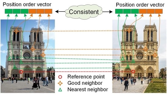
In this paper, we propose a new feature for each putative correspondence and use it in a learning-based method to identify incorrect matches. The observation is that for a correct match, the relative order for several of its neighbors should be stable from one view to another. By contrast, the difference between the relative order for the neighbors of an incorrect match will be obviously large. Following this idea, a feature vector representing the relative order difference for the neighbors of a reference correspondence is computed. However, such a feature is dependent on the direction of two images. That is, the features will be different when computed forward and backward. To remove the asymmetry, we first compute the feature vector from the first image to the second image and do the same thing in a reverse direction. Finally, we concatenate them to obtain a higher dimensional feature vector. Since this feature vector encodes the bidirectional local structure shift of a putative correspondence on both views, we name it the Mutual Structure Shift Feature (MSSF). Ideally, correct matches can better preserve the local structure, so they present a small ranking difference and tend to distribute near the origin of the MSSF space. In contrast, wrong matches will spread far away from the origin. In this way, inliers and outliers can be distinguished more clearly.
Another issue we are facing is how to define the local neighborhood when computing the proposed MSSF. Using spatially nearest neighbors is intuitive, but outliers might inevitably be involved. In this case, the feature of a correct match will shift towards the domain of incorrect matches along certain dimensions, making classification more difficult. A toy example is given in Figure 1. Figure 1a visualizes our MSSF by mapping it to a lower dimensional space when the neighborhood is contaminated by outliers. As we can see, there is significant overlap between positive and negative samples, making classification harder, while Figure 1b is the ideal case when the neighborhood contains no outliers. Compared with Figure 1a, the distributions of positive and negative samples are more compact and discriminative. The number of points mixed with a different class is also reduced. Inspired by the above observation, we make two improvements to our algorithm. First, we use geometrically “good” neighbors in conjunction with spatially nearest neighbors to reduce the risk of involving outliers. Second, we design an iterative weighting approach to enhance inliers and suppress outliers. Specifically, in each step, each neighboring correspondence is weighted by two scores: goodness and correctness. Goodness indicates whether a neighboring correspondence shares similar geometric properties with the target, and correctness reflects the confidence of a neighboring correspondence predicted by our model. As the iteration goes on, the weights of suspected mismatches gradually shrink, and the MSSF will be less affected by outliers. Finally, a random forest classifier trained with the proposed MSSF is used to distinguish correct matches from incorrect matches.
Briefly, the contribution of this paper lies in the following aspects. (1) We propose a novel Mutual Structure Shift Feature (MSSF) to better distinguish correct and incorrect matches. The main observation is that the neighbors of correct matches are more likely to have consistent rankings across different views. (2) We propose to combine geometrically “good” neighbors with spatially nearest neighbors, which reduces the risk of involving outliers. (3) We propose an iterative weighting strategy considering both goodness and correctness of a match to enhance inliers and suppress outliers. As a result, our feature shows good distribution property and is more friendly to the classification task.

2. Related Work

2.1. Traditional Methods

As a hot topic in computer vision, mismatch removal has been well studied in the past few years. Being one of the most famous robust model estimators, RANSAC and its variants [32,33,34] have been widely used in many modern applications such as SfM and SLAM. It estimates a parametric two-view geometry model in a re-sampling fashion, and removes correspondences with too large fitting errors. Different from an explicit binocular geometric model, ICF [35] learns two matching functions to check the consistency of putative matches in which each matching function regresses the position of a matching point from one image to another. However, the relationship between correspondences is somewhat ignored. In VFC [19] and its variants [18,20,36], correspondences are supposed to agree with a non-rigid motion function in a Bayesian framework. An additional regularization term is introduced to impose smoothness and coherence constraint. The unique global coherent restriction is extended by CODE [37] in which the non-linear regression formulation accommodates different local motion types with spatial discontinuities. Recently, the RFM [38] method has tried to find correct matches satisfying multiple local consistent motion patterns from a clustering view. The classical DBSCAN method is customized to achieve this goal.
To capture local motion properties, a method called LPM [23] was proposed. By computing k nearest neighbors of a correct match on both images, the authors required that two neighborhood sets should have a large intersection. This problem is formulated as a convex optimization problem with a closed-form solution, which is more computationally efficient than the aforementioned iterative methods. Later, the intersection of the k-nn measurement in the LPM was replaced with the weighted Spearman’s footrule distance in mTopKRP [39]. This work revealed that rank information of neighbors has the potential for distinguishing correct from wrong matches. However, our method differs from it in two major differences. First, mTopKRP chooses k nearest points on two views separately. As a result, two sets of neighbors may not belong to the same matches, making similarity measuring intractable. Second, it does not consider the quality of k nearest neighbors, which may involve outliers. By contrast, the proposed method selects neighboring correspondences rather than merely points in two directions and designs a weighting strategy to suppress outliers.

2.2. Learning-Based Methods

Apart from optimization-based methods, some researchers resort to learning algorithms to identify incorrect matches, which is essentially binary classification. Ma et al. [30] proposed a handcrafted feature for the classification task. Their combinatorial 33-dimensional feature fuses different attributes of a local neighborhood, such as percentage of intersection, ratio of length and angle. Moo Yi et al. [29] proposed the first work using deep learning, LGC. Inspired by the successful experience in point cloud processing, they designed an architecture based on Multi-Layer Perceptrons and ResNet blocks to extract features from each correspondence. Their training aims to minimize both classification loss and geometric loss. However, neighborhood information was not considered when extracting features. In a more recent work, NM-Net [31], the authors defined a graph around each correspondence and performed feature extraction with a graph convolution network. To avoid involving outliers in the graph, a good neighbor mining strategy was designed. Only classification loss was minimized because the structure constraint has already been integrated in the graph representation. This work was improved by CLNet [40], which progressively learns local-to-global consensus on dynamic graphs to prune outliers. To explore the complex context of putative correspondences, OANet [41] introduced a DiffPool layer and an Order-Aware DiffUnpool layer to capture local context. Moreover, it also developed order-aware filtering blocks to capture the global context. A novel smooth function which fits coherent motions on a graph of correspondences is proposed in LMCNet [42]. Based on its closed-form solution, a differentiable layer is designed in a deep neural network. ACN [43] is a simple yet effective technique to build permutation-equivariant networks. It normalizes the feature maps with weights estimated within the network, which can effectively exclude outliers.
Different from the above methods which rely on complicated principles or large networks, in this paper we propose a simpler yet effective feature to prune outliers, which measures the mutual structure shift between two views.

3. The Proposed Method

Suppose we have a pair of images I , I and an initial matching set C = c 1 , c 2 , c n between them. Each match c i consists of a pair of keypoints, i.e., c i = k i , k i , where k i comes from I, and k i comes from I . The position of a keypoint k i is represented by its image coordinate k i = x i , y i . Similarly, k i = x i , y i .

3.1. The Mutual Structure Shift Feature

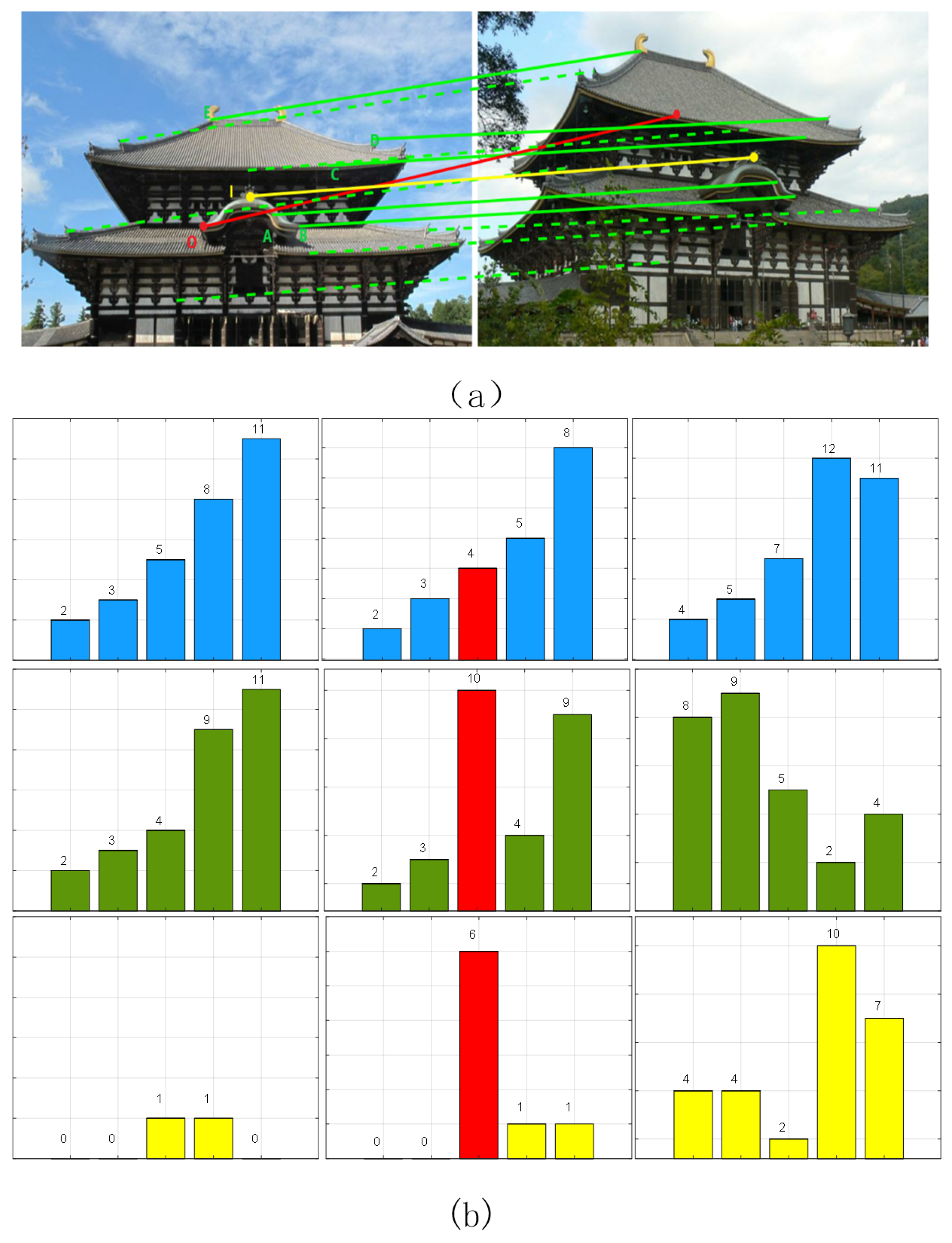
The basic idea of the proposed feature is that for a correct match, the relative order of its neighbors should be stable from one view to another, while this does not apply to outliers. Here we simply use the spatial Euclidean distance between keypoints as the distance measurement. Specifically, we compute the spatial distances between all the remaining points and the reference point and then sort them in an ascending order. Then, we record the distance orders for the selected neighbors. Let us have a look at an example shown in Figure 2. In Figure 2a, the red line represents a wrong match, and the remaining are correct matches. For a certain reference match, the three rows of Figure 2b plot the distance rankings of its neighbors on the first image, the second image and their difference, respectively. From left to right, we will discuss three cases. (1) We refer to I as the reference match and use its five correct neighbors { A , B , C , D , E } . (2) The same as (1), but we replace one of the above five correct neighbors with an outlier O (the red line). The neighbors are now { A , B , O , C , D } . (3) We consider an incorrect match O (the red line) as the reference and its five correct neighbors { A , B , C , D , E } . As we can see from the last row of Figure 2b, if the reference correspondence and all of its neighbors are correct, the two rankings are similar, and the order difference is the smallest. If the reference correspondence is correct but its neighbors are contaminated by outliers, the order difference will significantly increase at the corresponding position. If the reference correspondence is an outlier, the two rankings are quite different, and the order difference is generally larger. In this example, the order difference can help us to distinguish inliers from outliers. Since it implicitly encodes the structure information around the reference correspondence, we name it as the structure shift feature.
We denote the structure shift feature computed from I to I as f a and that computed from I to I as f b . Our mutual structure shift feature is a combination of f a and f b . Taking the former for an example, we first find neighbors of the reference correspondence on I and obtain the co-occurrence neighbors on I according to the correspondences. Denote N f as the distance order vector of the neighbors on I and N f as the distance order vector of the neighbors on I . Each element in the distance order vector is an integer in [ 1 , n 1 ] , where n is the total number of correspondences. Then, f a is defined as the absolute difference between the two order vectors, which can be expressed as:
f a = N f N f .
Equation (1) measures the change in the order of neighbor points. If the values in f a are closer to 0, the better structure is preserved. Similarly, f b can be computed in the same way in a reverse direction (from I to I).
Thus far, we have computed the structure shift feature for a reference correspondence f a and f b in both directions. Our mutual structure shift feature is then defined as:
f = f a f b ,
where ⊕ is the concatenation operation.

3.2. Neighbor Selection: Nearest Neighbors and “Good” Neighbors

As our mutual structure shift feature is built upon the neighbors of a reference correspondence, we need to carefully consider the neighbor selection strategy. Suppose the number of neighbors is k. Using k nearest neighbors in the Euclidean space is intuitive and easy to implement. However, such neighbors are vulnerable to mismatches, and the quality of the mutual structure shift feature decays significantly when the ratio of inliers is very low.
To address the above issue, we propose to adopt “good” neighbors instead of using spatially nearest neighbors only. In our context, “good” neighbors refer to those who share similar local geometric information with the reference correspondence. Specifically, we first use the Hessian detector to detects. The local 2 × 2 affine transformation matrices at a pair of matching keypoint k i and k i are denoted as A and A , respectively. Next, the geometric information matrix T i and T i for this correspondence are computed from the following equation:
T i = A i k i 0 1 , T i = A i k i 0 1 .
Then, we calculate the 3 × 3 local homography transformation at each keypoint using the following equation.
H i = T i T i 1 , H i = T i T i 1 , i = 1 , 2 , n ,
where H i maps k i to a new position in I , and H i maps k i to a new position in I. We assume that “good” neighbors should have the same or similar local homography transformation with each other.
Based on this assumption, we can compute the geometric consistency error between a pair of correspondences from:
e i j = σ ρ ( H j k i 1 ) ρ ( H i k i 1 ) ,
where i and j are the indices of two correspondences, ρ converts homogeneous coordinates into non-homogeneous coordinates, and σ returns the sum of absolute values of all the elements. Equation (5) indicates that if two keypoints k i and k j on image I are geometrically similar, the position after mapping k i with its own homography transformation H i should be close to the position after mapping it with H j , which is the homography transformation of k j . As a result, the geometric error e i j between keypoints k i and k j would be small. Similarly, e i j in Equation (6) reflects this property in a reverse direction. To regularize the errors to a particular interval, we compute a similarity score between any two correspondences by applying the following exponential mapping function:
s i j = e λ e i j + e j i , i , j = 1 , 2 , n ,
s i j = e λ e i j + e j i , i , j = 1 , 2 , n .
Here s i j and s i j indicate the similarities between correspondences i and j from I to I and from I to I, respectively. Both s i j and s i j range between [ 0 , 1 ] . According to [31], λ is a flexible parameter because it tunes the similarity values but does not change the ranking results. We set it to a constant 10 3 throughout this paper.
Finally, the neighbors of a reference correspondence c i = ( k i , k i ) consist of two kinds of neighbors, i.e., k nearest neighbors and k “good” neighbors. On the one hand, we find k nearest neighbors of both k i and k i on each image. On the other hand, we find the top k “good” neighbors on each image according to the similarity scores in Equation (7) and Equation (8). The mutual structure shift feature is computed from the union of these neighbors according to Equation (2). We can use these features to train a classifier to distinguish inliers from outliers.

3.3. Neighbor Weighting Strategy

In the previous neighbor selection stage, it is still difficult to avoid involving outliers. Hence, we design an iterative weighting strategy during testing to enhance inliers and suppress outliers in the neighborhood. At the very beginning, all the correspondences have the same weights so that they have equal chance to be chosen in the neighbor selection stage. In the following iterations, we first re-weight the correspondences given the prediction of the last iteration. Then, we compute new feature vectors based on the updated neighbors and feed them to the classifier. Please note that we only update features in each iteration, and the parameters of the random forest are fixed. The details of our iterative weighting strategy are as follows. When selecting nearest neighbors, we take the probability predicted by the classifier as the new confidence and select k nearest neighbors whose confidence is greater than a threshold. When selecting “good” neighbors, we use the following equation to re-weight the correspondences:
s i j ( q ) = s i j ( 0 ) p i ( q ) , i , j = 1 , 2 , n .
s i j ( q ) = s i j ( 0 ) p i ( q ) , i , j = 1 , 2 , n ,
where ∗ is the multiplication operator, s i j ( 0 ) and s i j ( q ) are the similarity scores initialized by Equation (7) and updated after the q t h iteration, respectively, and p i ( q ) is the probability of the i t h correspondence predicted by our classifier after the q t h iteration. In the next iteration, neighbors are selected using the above updated similarity scores. We can see from Equations (9) and (10) that if an outlier is involved by mistake at the beginning, it could be removed in the following process as the confidence predicted by the classifier gradually reduces.
Finally, a random forest classifier trained with the proposed MSSF feature is used to distinguish correct matches from incorrect matches. In our experiments, we use 40 decision trees in the forest. If the probability predicted by the classifier is greater than a threshold α , the correspondence is deemed correct.

4. Experiments

4.1. Datasets and Settings

Four public datasets were used in our experiments: DTU [44], DAISY [45], ChallengeData [46] and NMNET [31]. DTU is widely used for stereo matching. Images in each scene were taken at 49 or 64 different positions. The projection matrix of each view is provided as the ground truth. We used two recommended scenes scan1 and scan6 in our experiments. Each of them contained 180 image pairs. DAISY is a wide-baseline dataset which contains two scenes: fountain and herzjesu. There are 11 and 8 images in each scene, respectively. We created a total of 40 and 22 image pairs in each scene by matching adjacent images. Both the intrinsic and extrinsic parameters of each view are provided for evaluation. ChallengeData is designed for large scale Structure from Motion (SfM). Images in this dataset present different illumination, wide baseline and heavy occlusion, etc. The camera pose information reconstructed by a standard SfM pipeline [47] is provided as the ground truth. To surmount the excessive number of image pairs in this dataset, we selected three scenes: trevi_fountain, grand_place_brussels and hagia_sophia_interior for testing. Following the same protocol in [16], image pairs in each scene were classified into three categories according to the rotation angle: easy ([15 , 30 )), moderate ([30 , 45 )) and hard ([45 , 60 ]). For each category, we randomly selected 100 image pairs for testing. Finally, we used the NMNet dataset to test our application on Unmanned Aerial Vehicle (UAV) images. This dataset was captured by a drone at four sites. For each site, there are two versions of data: wide baseline and narrow baseline. In our experiment, we used the more challenging wide baseline version and selected 10 image pairs from each site. To determine if a correspondence was correct, we checked if the Epipolar geometric distance error was below a threshold γ . The default value of γ was two.
The proposed method was evaluated in two aspects. First, we employed precision (P), recall (R) and F1-score to see the raw matching quality. Moreover, we also report the F1-score, which was computed from:
F 1 = 2 P R P + R 100 % .
As we can see from Equation (11), the F1-score is a composite indicator of both precision and recall. Next, we also testes the accuracy of camera pose estimation, which is an important downstream task of feature correspondences. The performance was evaluated by the pose estimation accuracy. To be specific, we estimated the essential matrix between two views and recovered the rotation matrix R and translation vector t between them. Then, we measured the angle error by comparing the estimation with the ground truth using the following equations.
θ = arccos T r R p r e d T R g t 1 2 180 π , β = arccos t p r e d T t g t t p r e d t g t 180 π .
In Equation (12), the subscript p r e d and g t represent the estimated value and the ground truth, respectively; θ and β are the angle errors of the rotation matrix and the translation vector. In our experiments, the thresholds for both θ and β were set to 10 .
We compared our approach with six mismatch elimination algorithms from recent years. These includes traditional methods, such as LPM [23], mTop [39], RANSAC [32] and RFM [38], and modern machine-learning-based methods, such as LMR [30] and LGC [29]. All the experiments were performed on a machine equipped with a Xeon E5-2680 CPU, 64GB RAM and a GeForce GTX 1080Ti GPU.

4.2. Parameter Analysis

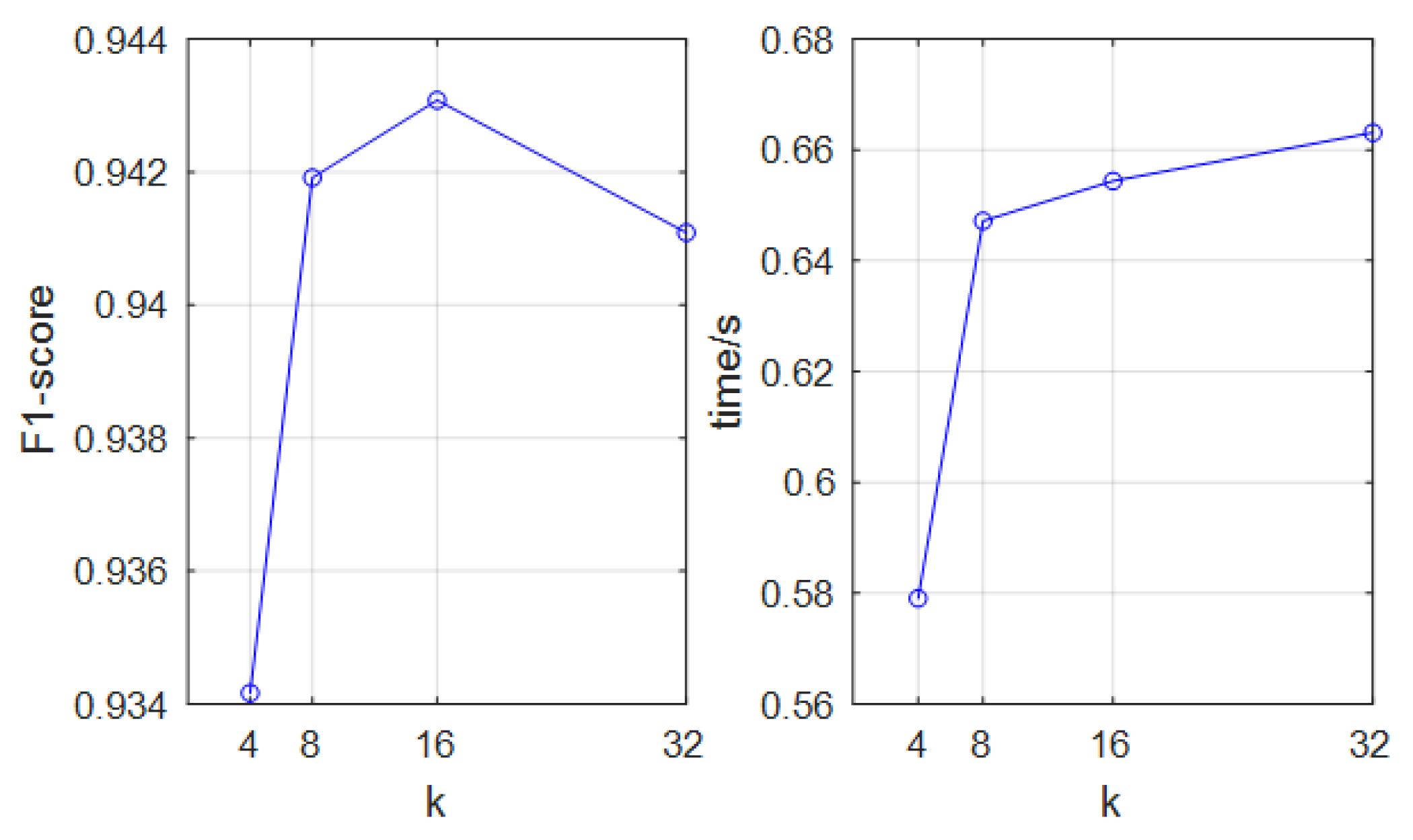
The size of neighborhood k is an important parameter in our method. It directly determines the dimension of the feature vector. On the one hand, smaller k not only limits the capacity of structure information in the feature, but also is sensitive to outliers and large deformation. On the other hand, larger k increases the risk of involving outliers in the neighborhood and will take up more resources as well. Hence, we analyzed k quantitatively by measuring the average F1-score and average running time on one of the scenes in ChallengeData. As shown in Figure 3, when k takes 4, 8, 16 and 32, the average F1-score first increases and then drops. Meanwhile, the average running time of each image pair keeps rising. To balance the two factors, we set k to 16 for all the experiments.
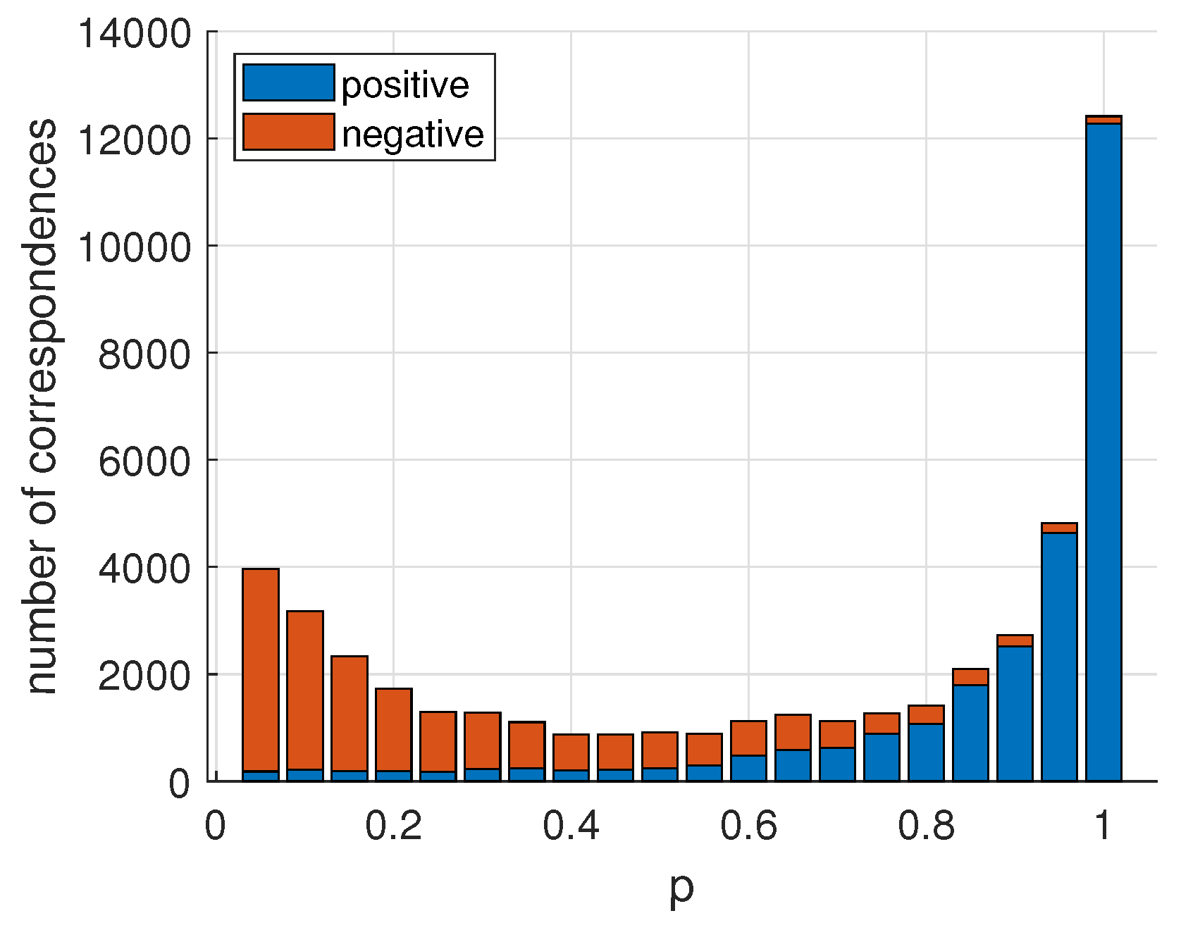
Another parameter to be investigated is the threshold α of the predicted probability. Generally speaking, increasing α can eliminate more outliers (leading to higher precision) but may kill more correct matches by mistake (leading to lower recall). Similarly, using smaller α may result in lower precision and higher recall. To set a proper value for α , the distribution of the predicted probability for both correct and wrong correspondences were investigated. In the example shown in Figure 4, the number of correct and wrong correspondences are 28 k and 18 k, respectively. For more than 90 % of the correct correspondences, their probabilities are greater than 0.7. We also note that the number of wrong correspondences whose probabilities are smaller than 0.4 accounts for nearly 70 % of the total. This property is favored because two distributions have small overlap. In order to balance the matching accuracy between correct and wrong correspondences, α was set to 0.5 for all the experiments.

4.3. Ablation Study

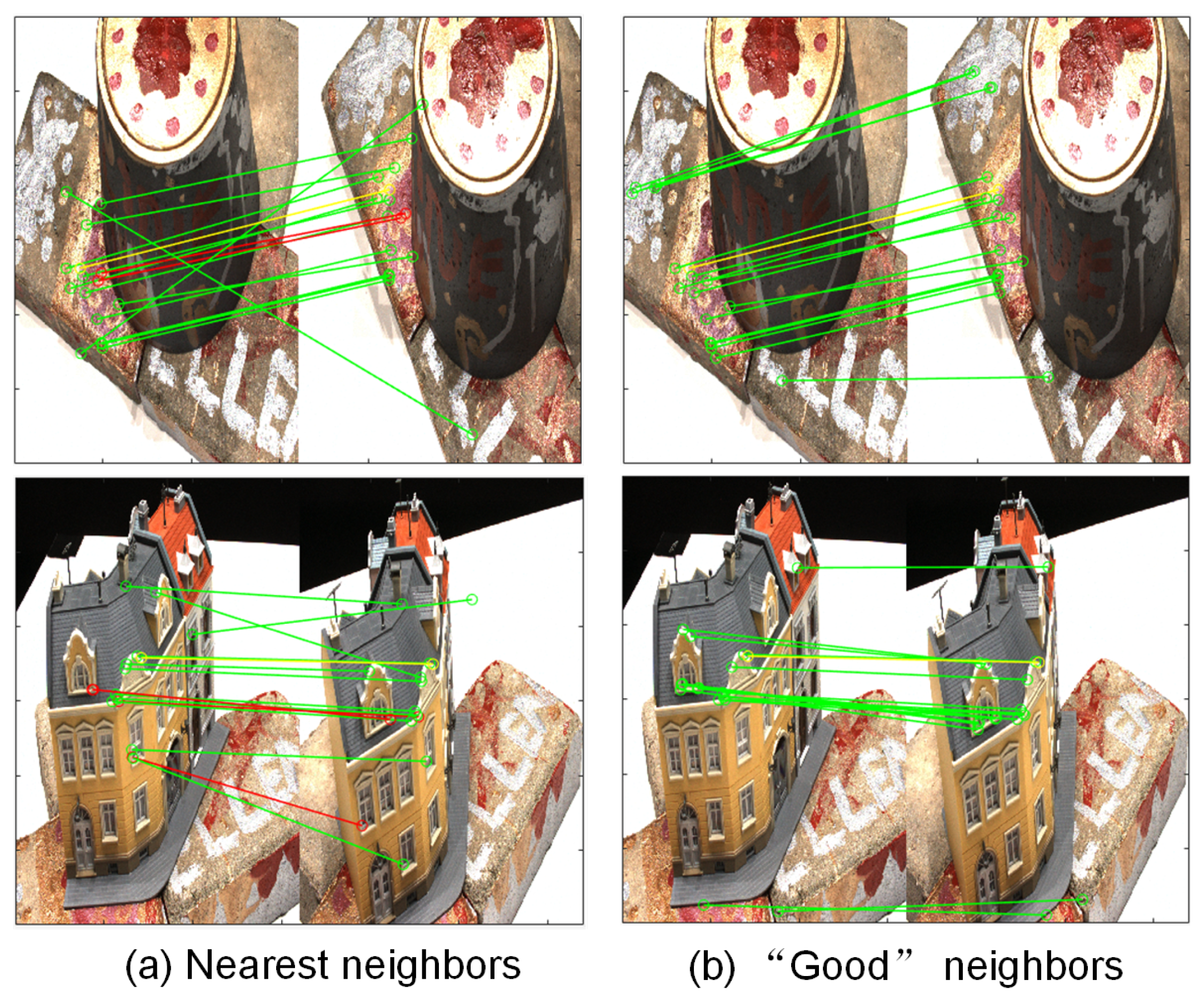
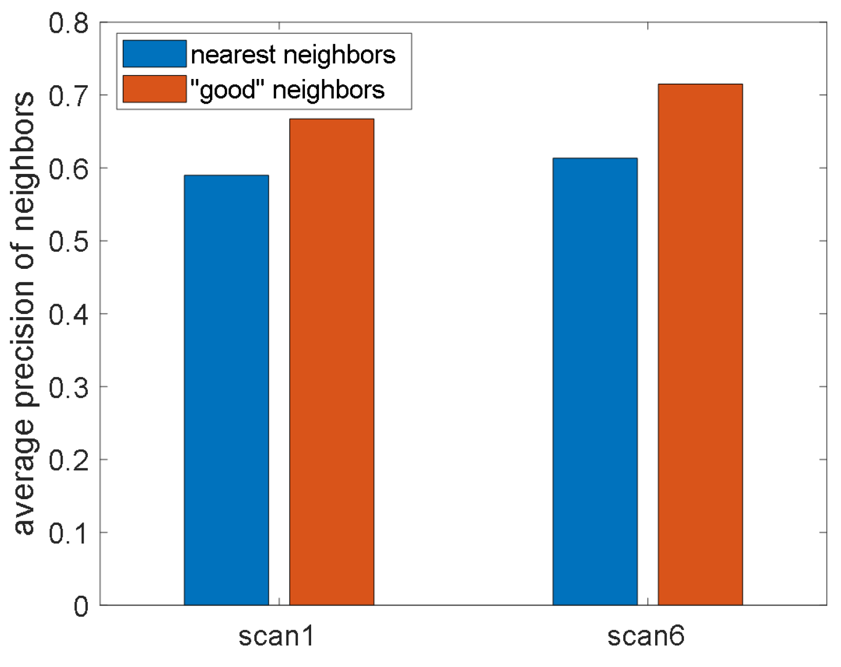
Different kinds of neighbors. The quality of neighbors is important. In the proposed method, we use the combination of both nearest neighbors and “good” neighbors. We also test the results of using nearest neighbors or “good” neighbors only. Thus, we use the DTU dataset to test the three settings and report the average F1-score in Table 1. As we can see, using the nearest neighbors is easy to implement and depicts the local structure well. However, it results in the lowest F1-score. The main reason is that nearest neighbors are easily contaminated by outliers. Using “good” neighbors only will increase the F1-score, which verifies that fewer outliers are involved by considering structure compatibility. The best results are achieved by using both nearest neighbors and “good” neighbors, which is shown in the last row. In Figure 5, we visualize both nearest neighbors and “good” neighbors on two pairs of images in the DTU dataset. As we can see, “good” neighbors are not always spatially nearby samples but contain fewer incorrect correspondences. Figure 6 plots the average precision of two kinds of neighbors on scan1 and scan6 of the DTU dataset. We can see that the average precision of “good” neighbors is significantly higher than nearest neighbors.
Mutual strategy. As stated before, measuring the structure shift is asymmetric with respect to the direction. That is, the results might be different when performing from I to I and from I to I. Hence, we adopt a mutual strategy which performs in both directions. Here we give the results with and without the mutual strategy in Table 2. Similar to Table 1, the average F1-scores on the DTU dataset are reported. It is worth noting that the mutual strategy will double the feature size and consume more resources. We can see that using a mutual strategy leads to better results. This shows that if it is hard to identify a mismatch in one direction, adopting the reverse direction makes up for it.
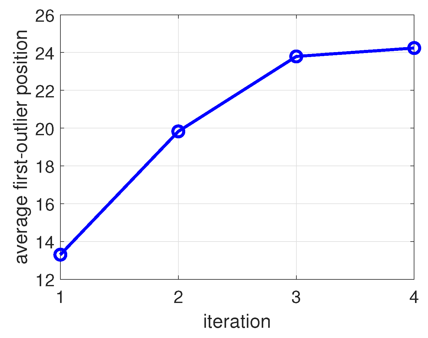
Iterative neighbor weighting strategy. In this part, we investigate whether the proposed iterative neighbor weighting strategy can truly reduce the risk for neighbors being contaminated by outliers. Hence, we define the First Outlier Position (FOP) as the indicator. FOP is a positive integer which indicates the position where the first outlier appears in the neighbor sequence. In other words, neighbors ranking before FOP are all inliers. Figure 7 shows the average FOP after each iteration for all the correspondences on a pair of images. As we can see, at the very beginning, the first outlier on average appears at the 13.3-th position in the neighbor sequence. This value grows up to 19.8 and 23.7 for the second and third iteration, respectively. If we run more iterations, the growth slows down. This curve shows that our weighting strategy pushes wrong correspondences to the back of the neighbor sequence. Thus, when we select the top k neighbors, the risk of involving outliers is greatly reduced. If k is smaller than the FOP, our neighbors will contain no outliers.

4.4. Raw Matching Quality Evaluation

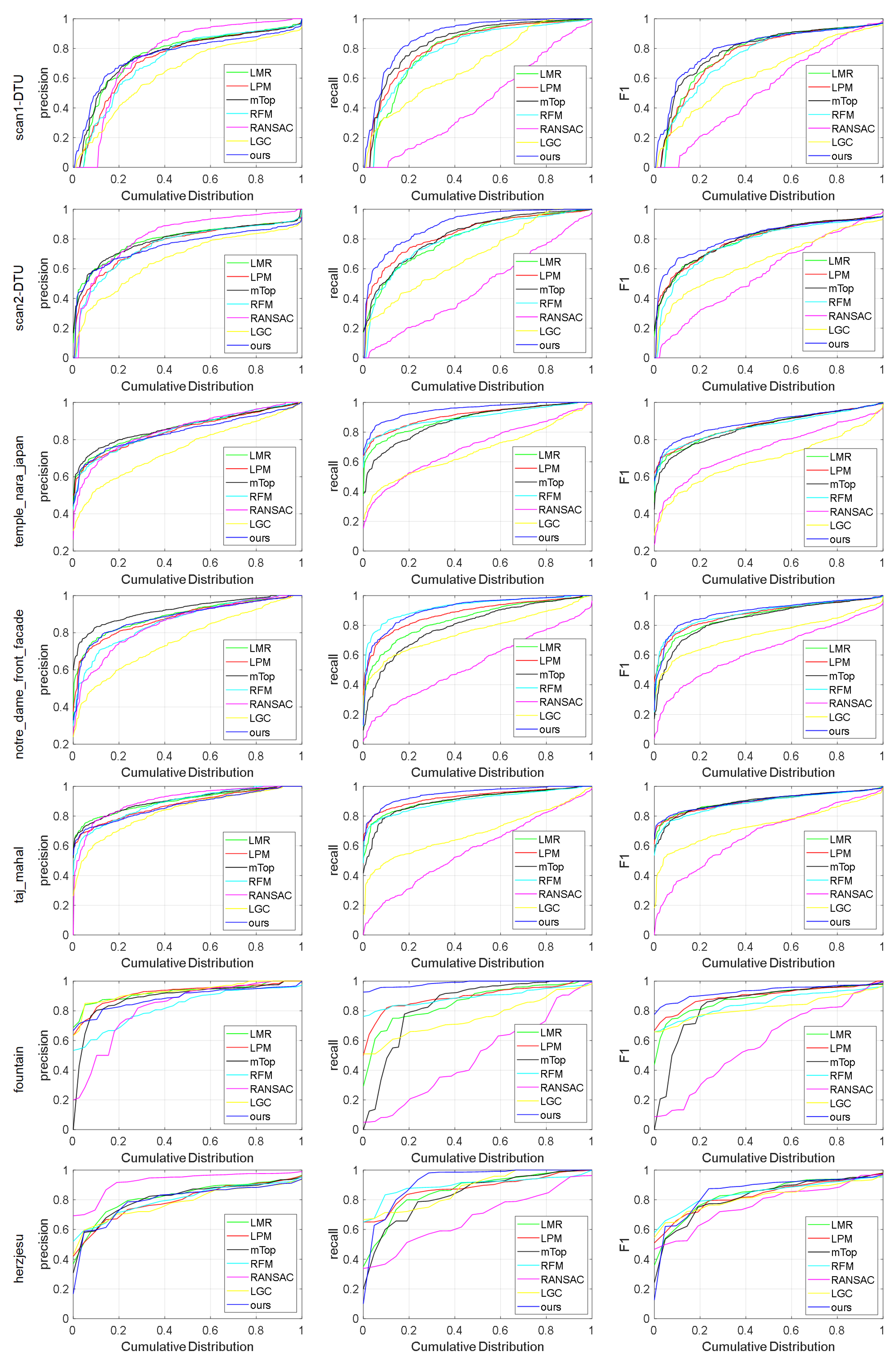
In order to verify the performance of our method, we calculate the average precision, recall and F1-score on seven scenarios from three datasets (two from DTU, three from ChallengeData and two from Daisy). For each scenario, we plot the cumulative distribution of precision, recall and F1-score for all image pairs in Figure 8. As we can see from this figure, the precision of our method is not always the best, but our recall is much higher than the other methods. As a result, our method has the best F1-score in most cases. This shows that our method can preserve correct correspondences as much as possible. We also note that for the first five scenes, there is not much difference between the F1-scores of different methods, except for RANSAC. However, it is even more significant for the last two scenes in Daisy. This shows that our method is superior to the other methods in generalization and stability.
In Table 3, we calculate the average F1-score with different thresholds τ for all the image pairs in Figure 8. As we can see, when τ increases from 0.5 to 4, our method achieves the highest F1-score all the time.

4.5. Pose Estimation Evaluation

Here, we evaluate the camera pose estimation accuracy of our method. We tested on two datasets: Daisy and ChallengeData. Daisy is a small-scale dataset, and the results are given in Table 4. As we can see, because of the very wide baseline in fountain, it is more challenging. and all the methods present lower accuracy than herzjesu. Our method has the highest accuracy for both translation and rotation. The gap between our method and the second best method is up to 5 % . ChallengeData contains 300 image pairs in total, which is much larger than Daisy. The results on this dataset are given in Table 5. As we can see, when the difference between cameras increases (from easy to hard in each scene), the performance drops consistently. Similarly, our method obtains the best accuracy on both rotation and translation.

4.6. Application on UAV Images

Finally, we evaluate the proposed method on UAV images. We first report the average F1-score in Table 6. The data show that our method improves the results better than the other methods. Next, we conducted relative pose estimation on this dataset and report the average angle error in Table 7. We can see that for scenes whose average F1-scores are higher than 90 % , e.g., mao-wide and science-wide, the pose errors returned by all the methods could be no larger than 1 . However, the pose errors for the compared methods easily rise to double digits for main-wide, whose average F1-scores are obviously lower than the above two scenes. Our method has the lowest errors for all the scenes.

5. Conclusions

In this paper, we propose a new method to remove incorrect correspondences between two images. We found that for a correct reference correspondence, the distance rankings of its neighbors are consistent from one view to another. Based on this observation, we propose a new feature called the Mutual Structure Shift Feature (MSSF), which measures the bidirectional ranking difference for the neighbors of a reference correspondence. To compute MSSF, we combine both spatially nearest neighbors with geometrically consistent neighbors. In this way, the risk of involving outliers in the neighbors is effectively reduced. We also design an iterative weighting strategy to progressively enhance correct correspondences and suppress incorrect correspondences. Extensive experiments on both raw matching quality evaluation and downstream tasks are carried out, showing our method outperforms the other compared methods.
In spite of the advantages, the limitations of our method lie in the following aspects. Firstly, since our method relies on information from the neighbors, its performance may deteriorate when we are not able to find enough qualified neighbors. This usually happens when the initial correspondences are too sparse or the inlier ratio is extremely low. Secondly, although our iterative weighting strategy can effectively exclude outliers in the neighbors, it cannot remove incorrect correspondences that are associated with high confidence by the model at the very beginning. That is, if an incorrect correspondence could not be clearly recognized in the early stage, it is harder to identify it later.

Author Contributions

Conceptualization, J.L. and K.S.; methodology, K.S. and K.L.; software, J.L.; validation, J.L.; formal analysis, S.J., K.L. and W.T.; resources, S.J.; writing—original draft preparation, K.S.; writing—review and editing, K.S. and K.L.; visualization, J.L. and S.J.; supervision, K.S. and W.T. All authors have read and agreed to the published version of the manuscript.

Funding

This work was supported by the National Natural Science Foundation of China No. 62176242 and No. 62176096, also in part by the National Natural Science Foundation of China No. 61906177 and No. 42001413.

Data Availability Statement

The data presented in this study are openly available in [31,44,45,46].

Conflicts of Interest

The authors declare no conflict of interest.

References

  1. Ma, J.; Jiang, X.; Fan, A.; Jiang, J.; Yan, J. Image Matching from Handcrafted to Deep Features: A Survey. Int. J. Comput. Vis. 2020, 129, 23–79. [Google Scholar] [CrossRef]
  2. Ma, X.; Xu, S.; Zhou, J.; Yang, Q.; Yang, Y.; Yang, K.; Ong, S.H. Point set registration with mixture framework and variational inference. Pattern Recognit. 2020, 104, 107345. [Google Scholar] [CrossRef]
  3. He, Q.; Zhou, J.; Xu, S.; Yang, Y.; Yu, R.; Liu, Y. Adaptive Hierarchical Probabilistic Model Using Structured Variational Inference for Point Set Registration. IEEE Trans. Fuzzy Syst. 2020, 28, 2784–2798. [Google Scholar] [CrossRef]
  4. Wang, T.; Jiang, Z.; Yan, J. Clustering-aware Multiple Graph Matching via Decayed Pairwise Matching Composition. In Proceedings of the Thirty-Fourth AAAI Conference on Artificial Intelligence, New York, NY, USA, 7–12 February 2020. [Google Scholar]
  5. Wang, R.; Yan, J.; Yang, X. Combinatorial Learning of Robust Deep Graph Matching: An Embedding based Approach. IEEE Trans. Pattern Anal. Mach. Intell. 2020. early access. [Google Scholar] [CrossRef]
  6. Min, J.; Lee, J.; Ponce, J.; Cho, M. Hyperpixel flow: Semantic correspondence with multi-layer neural features. In Proceedings of the IEEE International Conference on Computer Vision, Seoul, Republic of Korea, 27 October–2 November 2019; pp. 3395–3404. [Google Scholar]
  7. Tang, L.; Deng, Y.; Ma, Y.; Huang, J.; Ma, J. SuperFusion: A Versatile Image Registration and Fusion Network with Semantic Awareness. IEEE CAA J. Autom. Sin. 2022, 9, 2121–2137. [Google Scholar] [CrossRef]
  8. Lowe, D.G. Distinctive Image Features from Scale-Invariant Keypoints. Int. J. Comput. Vis. 2004, 60, 91–110. [Google Scholar] [CrossRef]
  9. Bay, H.; Tuytelaars, T.; Gool, L.V. SURF: Speeded Up Robust Features. In Proceedings of the European Conference on Computer Vision, Graz, Austria, 7–13 May 2006; Lecture Notes in Computer Science. Springer: Berlin/Heidelberg, Germany, 2006; Volume 3951, pp. 404–417. [Google Scholar] [CrossRef]
  10. Calonder, M.; Lepetit, V.; Strecha, C.; Fua, P. BRIEF: Binary Robust Independent Elementary Features. In Proceedings of the European Conference on Computer Vision, Heraklion, Greece, 5–11 September 2010; Lecture Notes in Computer Science. Springer: Berlin/Heidelberg, Germany, 2010; Volume 6314, pp. 778–792. [Google Scholar] [CrossRef]
  11. Leutenegger, S.; Chli, M.; Siegwart, R. BRISK: Binary Robust invariant scalable keypoints. In Proceedings of the IEEE International Conference on Computer Vision, Washington, DC, USA, 20–25 June 2011; pp. 2548–2555. [Google Scholar] [CrossRef]
  12. Tian, Y.; Fan, B.; Wu, F. L2-Net: Deep Learning of Discriminative Patch Descriptor in Euclidean Space. In Proceedings of the IEEE Conference on Computer Vision and Pattern Recognition, Honolulu, HI, USA, 21–26 July 2017; pp. 6128–6136. [Google Scholar] [CrossRef]
  13. Mishchuk, A.; Mishkin, D.; Radenovic, F.; Matas, J. Working hard to know your neighbor’s margins: Local descriptor learning loss. In Proceedings of the Annual Conference on Neural Information Processing Systems, Long Beach, CA, USA, 4–9 December 2017; pp. 4826–4837. [Google Scholar]
  14. Dusmanu, M.; Rocco, I.; Pajdla, T.; Pollefeys, M.; Sivic, J.; Torii, A.; Sattler, T. D2-Net: A Trainable CNN for Joint Description and Detection of Local Features. In Proceedings of the IEEE Conference on Computer Vision and Pattern Recognition, Computer Vision Foundation, Long Beach, CA, USA, 15–20 June 2019; pp. 8092–8101. [Google Scholar] [CrossRef]
  15. Tian, Y.; Yu, X.; Fan, B.; Wu, F.; Heijnen, H.; Balntas, V. SOSNet: Second Order Similarity Regularization for Local Descriptor Learning. In Proceedings of the IEEE/CVF Conference on Computer Vision and Pattern Recognition (CVPR 2019), Long Beach, CA, USA, 16–20 June 2019; pp. 11016–11025. [Google Scholar]
  16. Wang, Q.; Zhou, X.; Hariharan, B.; Snavely, N. Learning Feature Descriptors Using Camera Pose Supervision. In Proceedings of the ECCV, Glasgow, UK, 23–28 August 2020; Springer: Berlin/Heidelberg, Germany, 2020; Volume 12346, pp. 757–774. [Google Scholar]
  17. Ranftl, R.; Koltun, V. Deep fundamental matrix estimation. In Proceedings of the European Conference on Computer Vision (ECCV), Munich, Germany, 8–14 September 2018; pp. 284–299. [Google Scholar]
  18. Ma, J.; Zhao, J.; Tian, J.; Bai, X.; Tu, Z. Regularized vector field learning with sparse approximation for mismatch removal. Pattern Recognit. 2013, 46, 3519–3532. [Google Scholar] [CrossRef]
  19. Ma, J.; Zhao, J.; Tian, J.; Yuille, A.L.; Tu, Z. Robust point matching via vector field consensus. IEEE Trans. Image Process. 2014, 23, 1706–1721. [Google Scholar] [CrossRef]
  20. Ma, J.; Wu, J.; Zhao, J.; Jiang, J.; Zhou, H.; Sheng, Q.Z. Nonrigid point set registration with robust transformation learning under manifold regularization. IEEE Trans. Neural Netw. Learn. Syst. 2018, 30, 3584–3597. [Google Scholar] [CrossRef]
  21. Liu, H.; Yan, S. Common visual pattern discovery via spatially coherent correspondences. In Proceedings of the 2010 IEEE Computer Society Conference on Computer Vision and Pattern Recognition, San Francisco, CA, USA, 13–18 June 2010; pp. 1609–1616. [Google Scholar]
  22. Lipman, Y.; Yagev, S.; Poranne, R.; Jacobs, D.W.; Basri, R. Feature matching with bounded distortion. ACM Trans. Graph. (TOG) 2014, 33, 1–14. [Google Scholar] [CrossRef]
  23. Ma, J.; Zhao, J.; Jiang, J.; Zhou, H.; Guo, X. Locality preserving matching. Int. J. Comput. Vis. 2019, 127, 512–531. [Google Scholar] [CrossRef]
  24. Bian, J.; Lin, W.Y.; Matsushita, Y.; Yeung, S.K.; Nguyen, T.D.; Cheng, M.M. Gms: Grid-based motion statistics for fast, ultra-robust feature correspondence. In Proceedings of the IEEE Conference on Computer Vision and Pattern Recognition, San Juan, PR, USA, 17–19 June 2017; pp. 4181–4190. [Google Scholar]
  25. Liu, H.; Zheng, C.; Li, D.; Zhang, Z.; Lin, K.; Shen, X.; Xiong, N.N.; Wang, J. Multi-perspective social recommendation method with graph representation learning. Neurocomputing 2022, 468, 469–481. [Google Scholar] [CrossRef]
  26. Lhuillier, M.; Quan, L. Image Interpolation by Joint View Triangulation. In Proceedings of the 1999 IEEE Computer Society Conference on Computer Vision and Pattern Recognition, Fort Collins, CO, USA, 23–25 June 1999; pp. 2139–2145. [Google Scholar]
  27. Lee, I.C.; He, S.; Lai, P.L.; Yilmaz, A. BUILDING Point Grouping Using View-Geometry Relations. In Proceedings of the ASPRS 2010 Annual Conference, San Diego, CA, USA, 26–30 April 2010. [Google Scholar]
  28. Takimoto, R.Y.; Challella das Neves, A.; de Castro Martins, T.; Takase, F.K.; de Sales Guerra Tsuzuki, M. Automatic Epipolar Geometry Recovery Using Two Images. IFAC Proc. Vol. 2011, 44, 3980–3985. [Google Scholar] [CrossRef]
  29. Moo Yi, K.; Trulls, E.; Ono, Y.; Lepetit, V.; Salzmann, M.; Fua, P. Learning to find good correspondences. In Proceedings of the IEEE Conference on Computer Vision and Pattern Recognition, Salt Lake City, UT, USA, 18–23 June 2018; pp. 2666–2674. [Google Scholar]
  30. Ma, J.; Jiang, X.; Jiang, J.; Zhao, J.; Guo, X. LMR: Learning a two-class classifier for mismatch removal. IEEE Trans. Image Process. 2019, 28, 4045–4059. [Google Scholar] [CrossRef]
  31. Zhao, C.; Cao, Z.; Li, C.; Li, X.; Yang, J. NM-Net: Mining reliable neighbors for robust feature correspondences. In Proceedings of the IEEE Conference on Computer Vision and Pattern Recognition, Long Beach, CA, USA, 15–20 June 2019; pp. 215–224. [Google Scholar]
  32. Fischler, M.A.; Bolles, R.C. Random sample consensus: A paradigm for model fitting with applications to image analysis and automated cartography. Commun. ACM 1981, 24, 381–395. [Google Scholar] [CrossRef]
  33. Chum, O.; Matas, J. Matching with PROSAC-progressive sample consensus. In Proceedings of the 2005 IEEE computer society conference on computer vision and pattern recognition (CVPR’05), San Diego, CA, USA, 20–26 June 2005; Volume 1, pp. 220–226. [Google Scholar]
  34. Tran, Q.H.; Chin, T.J.; Carneiro, G.; Brown, M.S.; Suter, D. In defence of RANSAC for outlier rejection in deformable registration. In Proceedings of the European Conference on Computer Vision, Florence, Italy, 7–13 October 2012; Springer: Berlin/Heidelberg, Germany, 2012; pp. 274–287. [Google Scholar]
  35. Li, X.; Hu, Z. Rejecting mismatches by correspondence function. Int. J. Comput. Vis. 2010, 89, 1–17. [Google Scholar] [CrossRef]
  36. Ma, J.; Zhou, H.; Zhao, J.; Gao, Y.; Jiang, J.; Tian, J. Robust feature matching for remote sensing image registration via locally linear transforming. IEEE Trans. Geosci. Remote Sens. 2015, 53, 6469–6481. [Google Scholar] [CrossRef]
  37. Lin, W.Y.; Wang, F.; Cheng, M.M.; Yeung, S.K.; Torr, P.H.; Do, M.N.; Lu, J. CODE: Coherence based decision boundaries for feature correspondence. IEEE Trans. Pattern Anal. Mach. Intell. 2017, 40, 34–47. [Google Scholar] [CrossRef]
  38. Jiang, X.; Ma, J.; Jiang, J.; Guo, X. Robust feature matching using spatial clustering with heavy outliers. IEEE Trans. Image Process. 2019, 29, 736–746. [Google Scholar] [CrossRef]
  39. Jiang, X.; Jiang, J.; Fan, A.; Wang, Z.; Ma, J. Multiscale locality and rank preservation for robust feature matching of remote sensing images. IEEE Trans. Geosci. Remote Sens. 2019, 57, 6462–6472. [Google Scholar] [CrossRef]
  40. Zhao, C.; Ge, Y.; Zhu, F.; Zhao, R.; Li, H.; Salzmann, M. Progressive Correspondence Pruning by Consensus Learning. In Proceedings of the ICCV, Montreal, BC, Canada, 11–17 October 2021; pp. 6444–6453. [Google Scholar]
  41. Zhang, J.; Sun, D.; Luo, Z.; Yao, A.; Chen, H.; Zhou, L.; Shen, T.; Chen, Y.; Quan, L.; Liao, H. OANet: Learning Two-View Correspondences and Geometry Using Order-Aware Network. IEEE Trans. Pattern Anal. Mach. Intell. 2022, 44, 3110–3122. [Google Scholar] [CrossRef]
  42. Liu, Y.; Liu, L.; Lin, C.; Dong, Z.; Wang, W. Learnable Motion Coherence for Correspondence Pruning. In Proceedings of the CVPR. Computer Vision Foundation, Virtual, 19–25 June 2021; pp. 3237–3246. [Google Scholar]
  43. Sun, W.; Jiang, W.; Trulls, E.; Tagliasacchi, A.; Yi, K.M. ACNe: Attentive Context Normalization for Robust Permutation-Equivariant Learning. In Proceedings of the CVPR. Computer Vision Foundation, Seattle, WA, USA, 14–19 June 2020; pp. 11283–11292. [Google Scholar]
  44. Aanæs, H.; Jensen, R.R.; Vogiatzis, G.; Tola, E.; Dahl, A.B. Large-Scale Data for Multiple-View Stereopsis. Int. J. Comput. Vis. 2016, 120, 153–168. [Google Scholar] [CrossRef]
  45. Tola, E.; Lepetit, V.; Fua, P. DAISY: An Efficient Dense Descriptor Applied to Wide-Baseline Stereo. IEEE Trans. Pattern Anal. Mach. Intell. 2010, 32, 815–830. [Google Scholar] [CrossRef]
  46. Jin, Y.; Mishkin, D.; Mishchuk, A.; Matas, J.; Fua, P.; Yi, K.M.; Trulls, E. Image Matching Across Wide Baselines: From Paper to Practice. Int. J. Comput. Vis. 2021, 129, 517–547. [Google Scholar] [CrossRef]
  47. Schönberger, J.L.; Frahm, J. Structure-from-Motion Revisited. In Proceedings of the CVPR, Las Vegas, NV, USA, 27–30 June 2016; pp. 4104–4113. [Google Scholar]
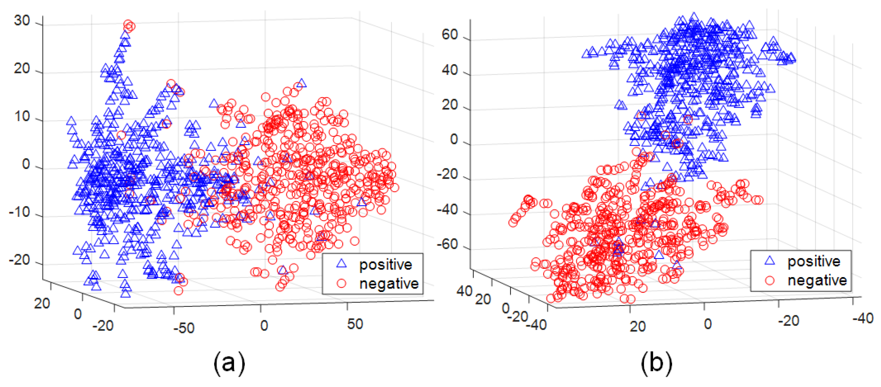
Figure 1. A visualization of the proposed MSSF after mapping it to a lower dimensional space: (a) computed features when the neighborhood contains outliers; (b) computed features when the neighborhood contains no outliers. Compared with (a), red points and blue points in (b) distribute more compactly, and the number of points mixed with another class is also reduced. This property is more in agreement with the consequent classification task.
Remotesensing 15 00926 g001
Figure 2. An example of the structure shift feature: (a) some correspondences on a pair of images; (b) from top to bottom: the distance rankings for the neighbors of a reference correspondence on the first image, the second image and their difference, respectively. From left to right: a correct reference correspondence (in yellow) with five correct neighbors (solid green lines), a correct reference correspondence (in yellow) with four correct neighbors (solid green lines) and a wrong neighbor point (solid red lines), a wrong reference correspondence (in red) with five correct neighbors (solid green lines).
Remotesensing 15 00926 g002
Figure 3. The analysis of k on grand_place_brussels from ChallengeData: Left: the average F1-score; Right: the average running time for each image pair.
Remotesensing 15 00926 g003
Figure 4. The probability distribution for both correct (blue) and wrong (red) correspondences in grand_place_brussels from ChallengeData.
Remotesensing 15 00926 g004
Figure 5. Visualization of both nearest neighbors and “good” neighbors on two pairs of images in the DTU dataset. The top row is from scan1 and the bottom row is from scan6. The reference correspondence is in yellow. Correct and wrong correspondences are in green and red, respectively.
Remotesensing 15 00926 g005
Figure 6. The average precision of both nearest neighbors and “good” neighbors on scan1 and scan2 in the DTU dataset.
Remotesensing 15 00926 g006
Figure 7. The average FOP after 4 iterations for all the correspondences on a pair of images.
Remotesensing 15 00926 g007
Figure 8. Results compared with several state-of-the-art methods. Each row is a scene. From top to bottom: scan1 and scan6 from DTU; temple_nara_japan, notre_dame_front_facade and taj_mahal from ChallengeData; fountain and herzjesu from Daisy. From left to right are: precision, recall and F1-score, respectively.
Remotesensing 15 00926 g008
Table 1. Ablation study of the neighbor selection strategy. The average F1-score (%) on the DTU dataset for three settings: using nearest neighbors only, using “good” neighbors only and using both of them. The best results are in bold.
Nearest Neighbors“Good” NeighborsScan1Scan6
-75.4380.23
-78.1781.38
78.9881.98
Table 2. Ablation study of the mutual strategy. The average F1-score (%) on the DTU dataset for two settings; w/o Mutual: using features computed from I to I only; w/Mutual: using features computed from both I to I and I to I. The best results are in bold.
SceneScan1Scan6
w/o Mutual79.2381.77
w/ Mutual79.9882.13
Table 3. The average F1-score (%) with different thresholds τ for all the image pairs in Figure 8. The best results are in bold. The red numbers in the brackets indicate the improvement between the best and the second best results.
ThresholdLMRLPMmTOPRFMRANSACLGCOurs
0.582.6282.1081.8878.6571.9175.2383.52 (+0.9)
184.5983.9083.7280.5472.3977.1886.01 (+1.42)
1.585.3084.6184.4581.4272.3777.8386.97 (+1.67)
286.0285.3685.2082.1772.2778.3887.86 (+1.84)
2.586.8385.9985.9283.1771.9779.2488.83 (+2.0)
387.3686.5086.3783.7171.6679.5589.34 (+1.98)
3.587.6986.8586.7684.1771.3479.9689.75 (+2.06)
487.8787.0786.9784.5071.0480.2390.07 (+2.2)
Table 4. Relative pose estimation accuracy (%) on Daisy. Each column represents a scene. Each cell represents the accuracy of rotation estimation (left) and the accuracy of translation estimation (right). The estimation of an image pair is successful when the angle error is under a certain threshold (10 ). The best results are in bold. The red numbers in the brackets indicate the improvement between the best and the second best results.
MethodFountainHerzjesu
LMR72.50/70.0090.91/90.91
LPM65.00/65.0086.36/86.36
mTOP70.00/70.0086.36/86.36
RFM67.50/67.5086.36/86.36
RANSAC57.50/55.0077.27/86.36
LGC57.50/55.0086.36/86.36
Ours75.00/75.00
(+2.5/+5.0)
95.45/95.45
(+4.54/+4.54)
Table 5. Relativepose estimation accuracy (%) on three scene of ChallengeData. Each cell represents the accuracy of rotation estimation (left) and the accuracy of translation estimation (right). The estimation of an image pair is successful when the angle error is under a certain threshold (10 ). The best results are in bold. The red numbers in the brackets indicate the improvement between the best and the second best results.
Methodtrevi_fountaingrand_place_brusselshagia_sophia_interior
EasyModerateHardEasyModerateHardEasyModerateHard
LMR98.0/88.097.0/90.092.0/88.095.0/61.084.0/59.078.0/63.096.0/35.088.0/60.085.0/77.0
LPM98.0/83.095.0/86.093.0/90.095.0/64.088.0/55.081.0/60.098.0/35.091.0/62.085.0/54.0
mTOP98.0/89.095.0/87.093.0/87.093.0/61.084.0/49.078.0/55.098.0/35.091.0/60.086.0/75.0
RFM98.0/85.087.0/81.090.0/83.093.0/56.081.0/52.076.0/64.096.0/35.089.0/59.084.0/76.0
RANSAC96.0/81.087.0/74.082.0/80.084.0/34.072.0/42.064.0/46.087.0/27.079.0/50.055.0/56.0
LGC92.0/77.078.0/68.076.0/73.090.0/49.076.0/47.064.0/48.094.0/30.087.0/49.064.0/56.0
Ours100.0/92.0 (+2.0/+3.0)99.0/92.0 (+2.0/+2.0)95.0/91.0 (+2.0/+1.0)96.0/66.0 (+1.0/+2.0)91.0/63.0 (+3.0/+4.0)84.0/73.0 (+3.0/+9.0)99.0/39.0 (+1.0/+4.0)95.0/64.0 (+4.0/+2.0)90.0/82.0 (+4.0/+5.0)
Table 6. The average F1-score (%) of four scenes from the NMNET dataset. The best results are in bold. The red numbers in the brackets indicate the improvement between the best and the second best results.
Lib-WideMain-WideMao-WideScience-Wide
LMR82.1174.4794.5891.44
LPM86.0876.5195.3693.09
mTOP85.4187.9095.2491.11
RFM86.7282.0694.7891.28
RANSAC49.7052.3583.6553.85
LGC81.2265.1292.4089.05
Ours90.33 (+3.61)92.67 (+4.77)96.75 (+1.39)94.26 (+1.17)
Table 7. The average rotation/translation angle errors ( ) on four scenes from the NMNET dataset. Smaller is better. The best results are in bold.
Lib-WideMain-WideMao-WideScience-Wide
LMR4.87/7.7413.09/18.810.12/0.900.20/0.60
LPM3.82/4.408.30/14.220.20/1.330.15/0.52
MTOP1.11/2.8511.93/21.030.16/1.240.18/0.61
RFM16.17/3.3910.84/24.100.14/1.210.16/0.52
RANSAC7.73/9.3218.15/14.850.39/2.320.38/1.54
LGC2.67/4.412.40/14.120.18/1.350.24/0.72
Ours0.45/1.331.22/13.170.10/0.840.11/0.36
Disclaimer/Publisher’s Note: The statements, opinions and data contained in all publications are solely those of the individual author(s) and contributor(s) and not of MDPI and/or the editor(s). MDPI and/or the editor(s) disclaim responsibility for any injury to people or property resulting from any ideas, methods, instructions or products referred to in the content.