Article

Cloud Removal from Satellite Images Using a Deep Learning Model with the Cloud-Matting Method

1
Faculty of Geosciences and Environmental Engineering, Southwest Jiaotong University, Chengdu 611756, China
2
School of Civil Engineering and Geomatics, Southwest Petroleum University, Chengdu 610500, China
*
Author to whom correspondence should be addressed.
Remote Sens. 2023, 15(4), 904; https://doi.org/10.3390/rs15040904
Submission received: 18 November 2022 / Revised: 30 January 2023 / Accepted: 4 February 2023 / Published: 6 February 2023

Abstract

:
Clouds seriously limit the application of optical remote sensing images. In this paper, we remove clouds from satellite images using a novel method that considers ground surface reflections and cloud top reflections as a linear mixture of image elements from the perspective of image superposition. We use a two-step convolutional neural network to extract the transparency information of clouds and then recover the ground surface information of thin cloud regions. Given the poor balance of the generated samples, this paper also improves the binary Tversky loss function and applies it on multi-classification tasks. The model was validated on the simulated dataset and ALCD dataset, respectively. The results show that this model outperformed other control group experiments in cloud detection and removal. The model better locates the clouds in images with cloud matting, which is built based on cloud detection. In addition, the model successfully recovers the surface information of the thin cloud region when thick and thin clouds coexist, and it does not damage the original image’s information.

1. Introduction

In recent years, optical satellite remote sensing has become the primary survey and monitoring means for disaster relief, geology, environment, and engineering construction, which has introduced great convenience to the development of human science. However, clouds are an unavoidable dynamic feature in optical remote sensing images. Global cloud coverage in mid-latitude regions is about 35% [1], and global surface cloud coverage ranges from 58% [2] to 66% [3]. High-quality images are not available almost all year round, especially in areas with high water vapor content changes [4]. Clouds reduce the reliability of remote sensing images and increase the difficulty of data processing [5].
Cloud detection is the first step in image de-clouding and restoration, which has received much attention from researchers. There are many methods concerning the detection of clouds and cloud shadows [6,7,8,9,10,11,12,13]. These methods can be divided into temporal and non-temporal solutions in terms of the number of images or non-deep learning solutions and deep learning [11,12,13,14] in terms of detection schemes. Foga et al. [15] summarized thirteen commonly used cloud detection methods and five cloud shadow detection methods. They found that the accuracy of each cloud removal method has its advantages and disadvantages within different scenarios. Deep learning-based methods mainly segment clouds in remote sensing images non-linearly with their solid-fitting ability. In the early years, scholars used fully connected neural networks [16,17] for cloud detection. In recent years, they primarily use convolutional neural networks [18,19] that are more suitable for image processing. Mahajan et al. [20] investigated the main cloud detection methods from 2004 to 2018, and they found that neural networks can largely compensate for the limitations of existing algorithms. The cloud detection scheme treats the detection process as a pixel classification, and it obtains a high-quality mask file but ignores the ground surface’s information under the cloud. In order to solve the problem in which the inaccurate mask file produces unsatisfactory results during cloud removal, Lin et al. [21] used the RTCR method and the augmented Lagrange multiplier. However, in most cases, the signals received by remote sensing imaging sensors are a superposition of the surface reflection signal and the cloud reflection signal [22,23]. Simple classification methods only locate and identify clouds in images but cannot estimate cloud amounts and recover surface information. Li et al. [24] suggested a hybrid cloud detection algorithm by utilizing various algorithms to their full potential. Clouds in images are usually mixed with surface information, and different transparency leads to different superposition patterns. Therefore, it is better to detect clouds by using a hybrid image element decomposition method.
Although there is a strong interconnection between cloud detection and cloud removal, studies have always been conducted separately [22,23]. Many scholars use deep learning techniques for single-image cloud removal. The widely used dark channel method has excellent mathematical derivations [25]. However, its applicability may be limited due to the imaging difference between satellite images and other images. Moreover, there are some errors in transmittance estimations and the dark channel prior, so the images are prone to dimming or are even distorted after cloud removal. The k-nearest neighbor (KNN) matting [26] method falls under nonlocal matting. It assumes that the transparency of a pixel can be described by weighting the transparency values of nonlocal pixels with a similar appearance, such as matching the color and texture. The goal is to allow the transparency value to propagate in nonlocal pixels. This includes laborious computations due to the comparison with the nonlocal images. KNN matting improves nonlocal matting by only considering the first K neighbors in the high-dimensional feature space. It reduces the amount of computation by only considering similarities between the color and the position in their feature space. The drawback of this method is that it requires a priori trimap as input and usually leaks pixels. Defining a general feature space with few parameters is difficult. Closed-form matting [27] assumes that the reflectivity of the foreground and background is the same in the local range of the sliding window and solves the transmittance formula using the color-line model and the ridge regression optimization algorithm. However, the clouds are easily overcorrected, and the solution requires an accurate trilateral as an a priori input, which significantly limits the application of closed extinction methods. The conditional generation countermeasure network (CGAN) [28] can reconstruct damaged information well when entities are still visible. However, the number of objects in remote-sensing images greatly increased. Therefore, the generative countermeasure network exhibits noticeable distortions in the thick cloud area. Isola et al. [29] proposed an image-to-image translation method (Pix2pix) based on CGAN to achieve image-to-image generation, providing a new method for image de-clouding restoration. Ramjyothi et al. [30] used GAN to repair the ground cover information under clouds in remote sensing images. Pan et al. [22] and Emami et al. [31] introduced spatial attention to GAN to control the redundancy of the model. Wen et al. [32] used a residual channel attention network for cloud removal. Via the solid-fitting ability of deep learning, the models can effectively learn the difference between the features of clouded and cloudless images, and then they can directly restore the absolute brightness value of the surface using image reconstruction. Cloud removal based on generative adversarial networks for reconstructing surface information is one of the trending research topics in recent years. However, the biggest drawback of deep learning is that “it cannot admit that it does not know when thin and thick clouds coexist”. The output of the models meets high metrics. However, there is a big difference between created images and real images. The commonly used cloud removal solutions for satellite images, especially for Sentinel-2, include Sen2cor [33], Fmask [34], and S2cloudless [35]. Qiu et al. introduced Global Surface Water Occurrence (GSWO) data based on Fmask3.3 and the global digital elevation model (DEM), and then proposed the use of Fmask4 to improve the accuracy by 7.2% compared to the Sen2cor algorithm specified by the European Space Agency (ESA) in version 2.5.5. Housman et al. proposed the cloud detection method S2cloudless by selecting ten bands of Sentinel-2 based on the XGBoost and LightGBM tree learning algorithms for model inference, which is the primary tool for Sentinel-hub cloud product production.
Other than the two-step “detection-removal” methods, Ji et al. [36] proposed a BC smooth low-rank plus group sparse model to detect and remove clouds at the same time.
Cloud removal methods for a single image rarely consider cloud transparency information. Surface information is often recovered approximately by interpolation or by mapping convolutional layers based on relevant samples. In most cases, the information about areas under thick clouds is completely lost. Cloud removal operations for such regions using interpolation or mapping methods introduce significant errors and sometimes result in useless images.
From the preceding description, this paper carries out experiments from a new cloud detection paradigm by simulating the mixing relationship between surface information and clouds, establishing a linear model based on the image superposition model. We propose an integrated method for cloud detection, transparency estimation, and cloud removal. This method can distinguish the foreground and background of mixed image elements based on single-band images in order to achieve cloud removal in a single satellite image. Considering that, the transparency of clouds varies in different bands of remote sensing images, the reflected signal of clouds in the RGB channel is the same, and the blue band is more sensitive to thin clouds. To promote the application of the model to multiple bands in order to enhance the applicability and generalization ability of the model, this paper uses the Sentinel-2 blue band for cloud-matting attempts. This idea mainly came from applying deep learning in image-matting methods, which assume that the image’s foreground and background are mixed by transparency information. The classic linear superposition formula is shown in Equation (1) [37]. Image I can be decomposed into a linear combination of foregrounds, F , and backgrounds, B:
I = α F + ( 1 α ) B , α [ 0 , 1 ]
where α is the cloud’s opacity ( α = [ 0 , 1 ] ). The convolutional neural network can acquire deeper feature information about the target [19], so the alpha matte of the foreground image estimated using the convolutional neural network can better remove the background information and extract the foreground information out of the image [38,39,40]. Given the poor balance of the generated samples, this paper also improves the binary Tversky loss function for multi-classification tasks. Through the improved Tversky loss function, we can automatically balance the weight of multi-class samples in the complex and changeable generated samples and focus the model’s attention on a specific class or multi-class samples. In this manner, we can improve the prediction results of hard segmentation, effectively distinguish thin and thick cloud regions, and recover cloud and shadow regions based on cloud transparency information.

2. Methodology

2.1. Remote Sensing Imaging Process

The cloud removal model proposed in this paper is a deep-learning-based assumption. Therefore, we simplify atmospheric transport operations by not considering the scattering of particles in the air as well as aerosols. As shown in Figure 1, cloud occlusion between the satellite and the ground surface results in a superposition between the reflected energy from the ground surface and the reflected energy from the cloud’s top in the final reflected energy obtained.
Different solar incidence angles form shadows that weaken or completely cover surface information. The pixel composition of the reflected signal intensity received by the remote sensing imaging system is as follows:
ε = ( 1 α ) ε g r o u n d + α ε c l o u d , ( a ) ε = ( 1 α ) ε g r o u n d , ( b )
where (a) represents the received reflective intensity of area with clouds and (b) represents the received reflective intensity of area with cloud shadows. α is the cloud opacity ( α = [ 0 , 1 ] ), ε g r o u n d is the reflection intensity at the surface, and ε c l o u d is the reflection intensity at the top of the cloud. Note that we assume constant solar irradiation with respect to clouds in the remote sensing image and a fixed cloud brightness (random sampling 4000–6000). Cloud brightness and transparency can be better balanced using sample generation based on Equations (1) and (2).

2.2. Model and Algorithm

The automatic generation of cloud-trimap is the first part of our proposed model, followed by the generation of a cloud-matting mask and cloud removal and, finally, the refinement and optimization of the cloud-matting mask and cloud removal’s result. Our model contains two convolutional networks, as shown in Figure 2. The first convolutional network (green) is the T-Net (Trimap generate network) and the other network (blue) is the M-Net (Matting network). The T-Net is a semantic segmentation model that detects clouds on satellite images. This model generates a cloud-trimap, which can classify the image into opaque clouds, transparent clouds (uncertain regions), and non-clouds. The M-Net is an end-to-end pixel estimation model that uses a multi-output method to fuse the model’s feature extraction results to estimate cloud transparency and residuals between the recovered and original images. Both T-Net and M-Net encoders adopt the Atrous spatial pyramid pooling (ASPP) structure at the bottom layer to represent more scaled information of image features with fewer parameters. The entire model can significantly improve prediction accuracies by model fusion and residual calculation. B, F, and U in Figure 2 represent the background, foreground, and conflicted regions, respectively. The output’s results are not activated using the Softmax function because the loss in the T-Net training process contains cross-entropy errors. We can obtain B S and U S by using the same method and, obviously, F S + B S + U S = 1 where 1 denotes the pixel value of each image element in the feature map.
F S = exp ( F ) exp ( F ) + exp ( B ) + exp ( U )
The output result of picking M-Net contains two parts. The first part, α r , mainly predicts the transparency information of clouds in the image. When the pixel is located in an uncertain region, this part is very likely to have transparent clouds. Otherwise, α r can be filtered.
α p = F S + U S α r
α p is the refinement of α r ; when U S shifts towards 1, then F S shifts towards 0. At the same time, α p shifts towards α r . When F S shifts towards 1, then U S shifts towards 0 and α p shifts towards F S ( α p 1 ). This simple filtering method can improve the prediction result’s confidence level. It also effectively shields background information interference and directs the model’s attention to the region where the image’s elements are mixed. The residuals between the predicted image and the cloud-free image are output by the M-Net, allowing the recovery of images using cloud transparency and the preservation of the original image’s features.
Taking the derivative of both sides of the Equation (1), we have the following.
B α = I F + ( 1 α ) I / α ( 1 α ) 2
From Equation (5), we can observe that when ( 1 α ) shifts towards zero, even a slight perturbation will result in a colossal mistake. The bottom map’s recovery is prone to distortion. Permitting M-Net to directly recover the original surface’s information—which is obscured by clouds—is unreliable without considering cloud transparency information. The prediction results need to be masked for regions with poor reliability (the mask’s threshold in Figure 2 is α 0.9 ). It is worth noting that the M-Net model’s input is the channel’s superimposed feature map of both the T-Net’s input and output, and Softmax is used to activate the T-Net’s output and project the feature value to [0,1].
Complex problems can be simplified by employing the two-step method. Compared to the commonly used one-step method, the two-step method can fix a portion of the parameters while training another portion, resulting in a smoother model optimization process and faster training convergence. Interpretability improves over time, resulting in more accurate predictions.
For both T-Net and M-Net, we adopt the classic end-to-end (Sequence to Sequence, Seq2Seq) structure, extract features via the encoder, and then fuse features via the decoder. Due to a large number of parameters in the T-Net, a residual connection is adopted. Since fewer parameters exist in the M-Net, the encoder and decoder channel stacking are adopted to minimize information loss between feature maps. The encoding and decoding process will still reduce the image’s sharpness when restored, so we will output the residuals to recover the image to the maximum extent.

2.3. Loss Function

The model is evaluated using a combined loss function.
Pre-training T-Net: Our T-Net primarily uses the cross-entropy error as the error function, according to Chen et al. [41]. The cross-entropy function is calculated using the following formula.
L c r o s s = i = 1 n x i log x ^ i
In Equation (6), [ x i , x ^ i ] denotes the pixel value of the predicted cloud-trimap and the real cloud-trimap, respectively. On the one hand, using only L c r o s s to generate cloud-trimap is unsatisfactory because T-Net’s input categories are unbalanced, and the output’s results are biased towards the background and conflicted regions, ignoring foreground information. On the other hand, due to the sample generation scheme used in the paper, it is challenging to add weights directly, making T-Net convergence difficult. The Tversky function was created to solve the problem of unbalanced medical image classification between focal and non-focal regions in machine learning by balancing the proportion of false positives and false negatives in training [42], resulting in a higher callback rate and a better balance between accuracy and sensitivity for the function. Therefore, we improve the binary classification Tversky function to solve the problem of unbalanced T-Net samples. In the binary classification problem, Tversky loss incorporates the benefits of focal loss [43] and Dice loss [44,45], and it is applied to the image segmentation study with the following formula transformation.
L T v e r s k y = 1 i = 1 n P x i P x ^ i + S i = 1 n [ ( 2 P x i + 1 ) ( 1 α 1 P x ^ i ) + α 1 P x i ] + S
In the neural network’s training process, P x i is the foreground probability of labeled pixels, P x ^ i is the foreground probability of predicted pixels, and α 1 is the weight of control parameters to balance the samples. We usually set 0 < S < 10 6 to ensure that the equation holds, and L T v e r s k y is the corresponding loss function.
The Tversky weight balance function is designed for binary classification problems and cannot directly apply to multiclassification problems. It is difficult to express the model error with a fixed weight because the first step of our model generates a cloud-trimap of images associated with multiple classifications. In addition, the trimap of each set of images is uncertain. In this paper, we improve the Tversky loss function by assuming that one or more classes of weights have a negative balance of significance. We build the automatic balance loss function with the classification corresponding to the unique thermal encoding channel.
T P k = k = 1 m 0 i = 1 n P x i k × P x ^ i k F P k = i = 1 n ( j = 1 m 1 P x i j × k = 1 m 0 P x ^ i k ) F N k = i = 1 n ( k = 1 m 0 P x ^ i k × j = 1 m 1 P x i j )
L T v e r s k y = 1 k = 1 m 0 T P k ( T P k + β F P k + ( 1 β ) F N k + S ) m 0 k = 1 n T P k > 0 L T v e r s k y = k = 1 m 0 F P k + F N k ( M × N ) m 0 k = 1 n T P k = 0
In Equations (8) and (9), m 0 is the image channel of interest after one-hot encoding; m 1 is the remaining channels included in the one-hot encoding; n is the number of pixels of the image; [ P x , P x ^ ] corresponds to the predicted classification and labeled classification, respectively; k and j represent the kth channel and jth channel of the image, respectively; β is the weight balance parameter; [ T P k , F P k , F N k ] denotes the true positive rate, false positive rate, and false negative rate of the attention channel, respectively; [ M , N ] is the training sample size of the image; L T v e r s k y is the loss value; S is the factor that prevents the denominator from proceeding to zero.
We effectively extend the dichotomous classification method to multi-categorization scenario applications by improving the Tversky loss function. The method does not require obtaining the sample’s share in advance. It can automatically balance the sample’s weights based on the samples’ distribution characteristics, which can still effectively adjust the model’s attention in the case of there being significant differences in the number of multi-categorization samples, ensuring that the model’s optimization process does not favor the more dominant category.
It is worth noting that when T P k is 0, the loss function L T v e r s k y degrades significantly. To compensate for the loss in model training, we concentrate on optimizing the loss function’s balance to be applied to any multiclassification model. To compensate for the model’s training degeneracy, we focus on optimizing the loss function’s balance to increase its applicability. L T v e r s k y directs the gradient optimizer towards the channel of interest for iterative optimization using the improved Tversky loss function. As the number of training increases, the number of false positives increases. The L T v e r s k y gradient direction shifts to reduce both false positives and false negatives for iterative optimizations. The T-Net loss function is calculated by adding L c r o s s and L T v e r s k y .
L T N e t = 0.5 ( L c r o s s + L T v e r s k y )
Freeze T-Net and training M-Net: we fixed the weight of the T-Net network to train the M-Net after several rounds of iterative T-Net output results converged. The final output of the model contains two parts: cloud transparency estimation, α p , and the recovered image, I p r e . We express the accuracy of α p as L | | α | | 2 and the reconstruction error as L c . The multi-scale expression of the distribution of L m s s s i m and the image element error in terms of I p r e are included. The α p error function can be expressed as follows.
L | | α | | 2 = i = 1 n ( x i x ^ i ) 2
L c = i = 1 n ( c i c ^ i ) 2
In Equations (11) and (12), [ x i , x ^ i ] represents the pixel values of predicted α p and actual α , respectively, and [ c i , c ^ i ] represents the pixel values of the synthetic cloud removal image and the actual cloud-free remote sensing image pixel values, respectively. The synthetic cloud removal image is generated from the actual background image and α p , according to Equation (1).
We introduce MS-SSIM as the I p r e error function; MS-SSIM is an image quality evaluation method that merges image details at different resolutions. It can evaluate two images based on their brightness, contrast, and structural similarity. The MS-SSIM loss function is calculated as shown in Equation (13).
L m s s s i m = 1 m = 1 M 2 μ p μ g + c 1 μ g 2 + μ g 2 + c 1 β m 2 σ p g + c 2 σ p 2 + σ g 2 + c 2 γ m
M represents the scale factor, [ μ p , μ g ] denotes the mean value between the predicted feature map and the actual image, [ σ p , σ g ] denotes the standard deviation between the predicted image and the actual image, σ p g denotes the covariance between the predicted image and the actual image, [ β m , γ m ] denotes the importance between the two multiplicative terms, and [ c 1 , c 2 ] is a constant term used to prevent the divisor from being 0. It is worth noting that the cloud occupation is usually tiny in remote sensing images. Therefore, the loss value obtained by calculating the global error function is small and cannot guide the optimization correctly.
We record the cloud-trimap output by the T-Net as the weight of the loss function, ω , to solve the problem that M-Net’s error cannot be optimized to calculate the feature mat’s local error (reduce the background error weight). Therefore, the L m s s s i m error function is [ μ p , μ g , σ p , σ g , σ p g ] = ω [ μ p , μ g , σ p , σ g , σ p g ] . As shown in Equation (14), the M-Net loss function combines the error functions of L | | α | | 2 , L c , and L m s s s i m . w denotes the significant coefficient, which ensures that the image is similar to the actual image and promotes the image’s element value to be more similar, and it will decrease as the number of iterations increases.
L M N e t = w ( L | | α | | 2 + L c ) + ( 1 w ) L m s s s i m

3. Experiments

3.1. Datasets

Existing cloud datasets are primarily designed for cloud detection, and they are accompanied by a mask for distinguishing clouds from other regions, which cannot be used for cloud-matting operations. As a result, we need simulated remote sensing cloud images as the model’s data driver. Therefore, in this paper, we refer to traditional matting sample generation cases such as the alphamatting.com dataset [46], portrait image matting dataset [47], classical remote sensing image cloud detection dataset, L7Irish [48], and L8SPARCS [49]. Cloud-matting samples were obtained from the blue band of the Sentinel-2 satellite, and the samples were pooled into one image as the actual label of cloud transparency; the cloud-free Sentinel-2 blue band image was used as the base image according to Equation (1) to build the training and validation dataset required for the study.
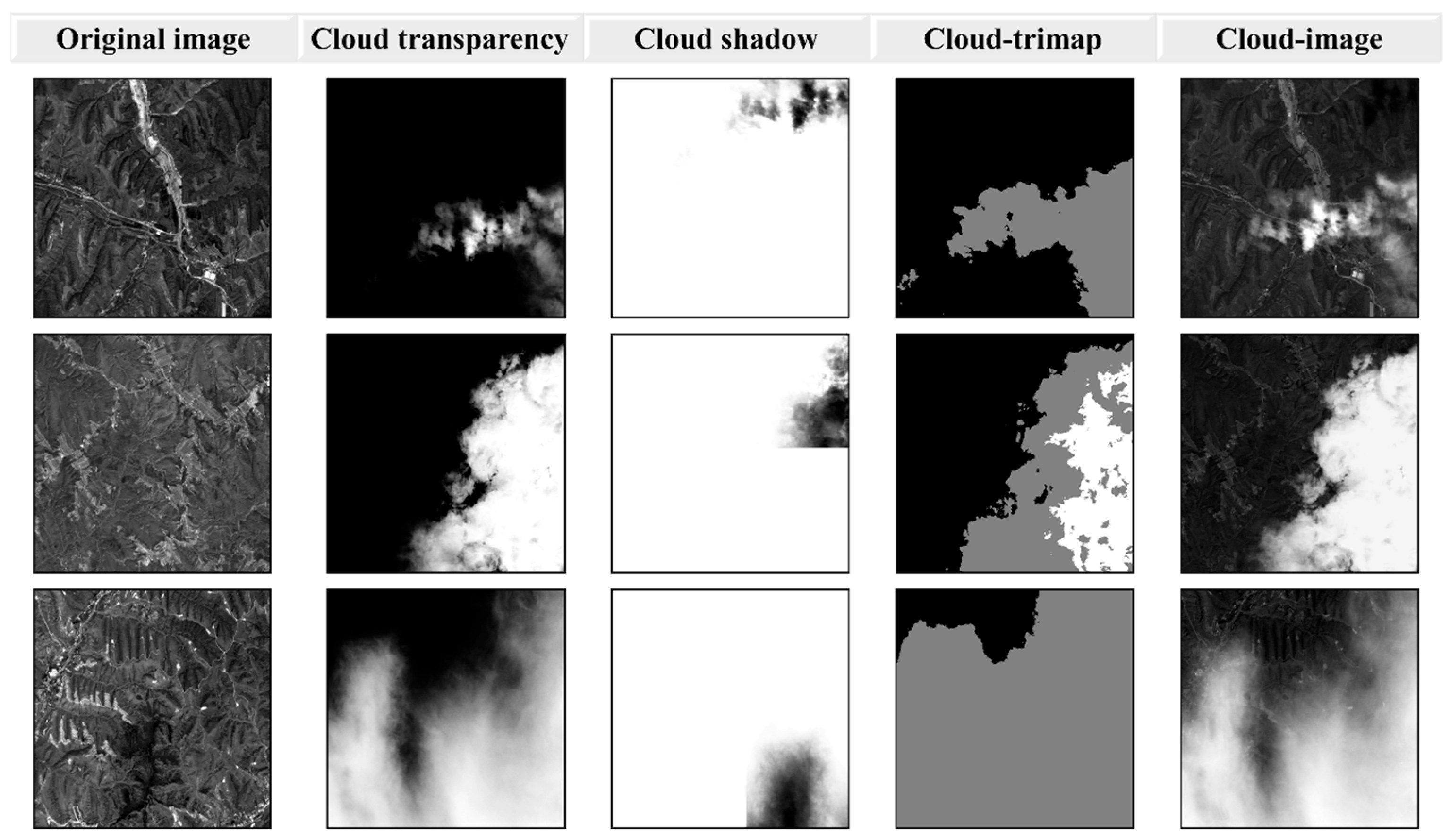
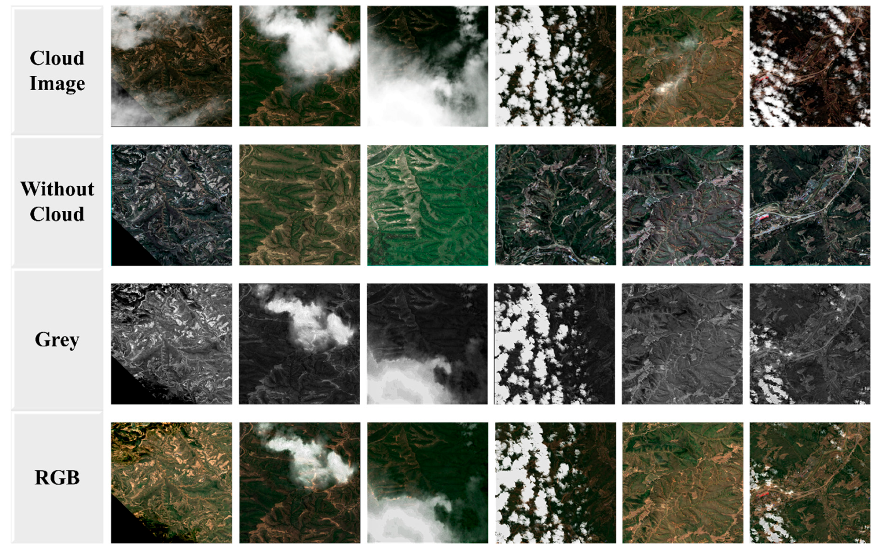
We used Equation (2) to assume that the absolute brightness of clouds is consistent within a specific range, and the cloud’s transparency primarily determines the variation of cloud light and darkness; thus, at first, we used the Sentinel-2 images from the sea to produce a normalized alpha layer based on the color range. We created a cloud-trimap based on the transparency threshold and added an offset (50–150 pixels) to simulate cloud shadows on this foundation. Secondly, we selected multi-scene Sentinel-2 images with few clouds in different areas and at different times. Then, we used a slice index to rank and build a cloudy area mask one by one in order to obtain a cloud-free remote sensing image base map. Thirdly, the base image was randomly cropped to the specified size, and then training and validation samples were generated using the cloud transparency image, shadow image, and random cloud brightness. Finally, we generated a total of 50,000 samples, of which 20% were used as the validation set, 5% were used as the prediction set, and 75% were used as the training set. Figure 3 depicts the dataset construction scheme and the result.
Cloud-trimap is obtained using a 3 × 3 sliding window image expansion calculation method based on cloud transparency. This aims to increase the tolerance of cloud detection by incorporating all information on image elements that may be clouded into cloud-trimap, and then they are further discriminated by the M-Net.

3.2. Evaluation Metrics

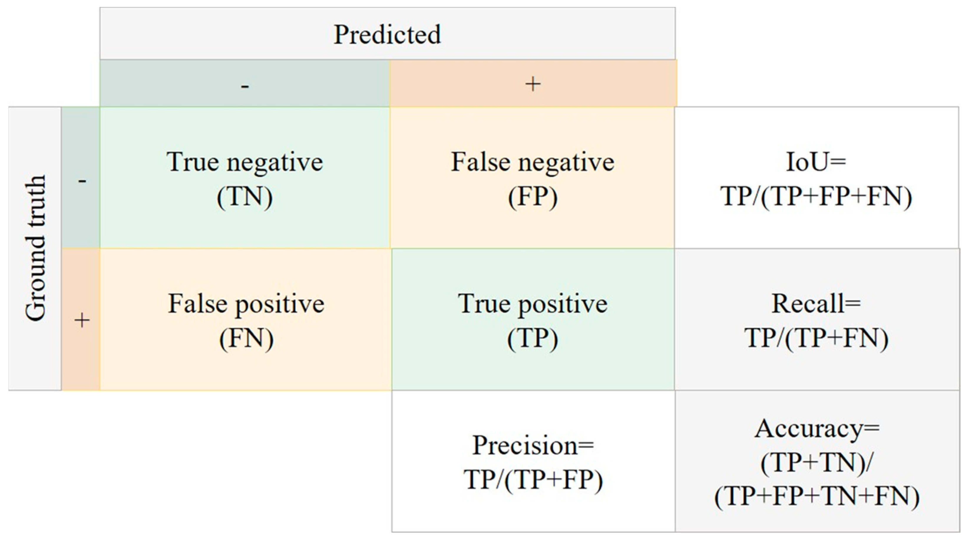
Our evaluation task involves cloud detection and cloud removal. The confusion matrix statistics of precision, recall, and accuracy were used for the former. The specific calculation is shown in Figure 4. For the latter, we used two methods to verify the results. 1. RMSE is used to verify the accuracy of the alpha calculation directly, and 2. SSIM is used to calculate the difference between the structural features of the predicted image and the real image. 3. The peak signal-to-noise ratio (PSNR) is also used. 4. The root mean square error (RMSE) is used to directly count the pixel difference between the predicted and actual images.

3.3. Implementation Details Evaluation Metrics

We compared and validated the cloud-matting method against the generated dataset and the Sentinel-2 classification dataset ALCD established by Baetens et al. [50]. For better verification, we also used three cloud detection methods and four de-clouding algorithms to demonstrate its effectiveness.
The cloud detection methods used for comparisons include S2cloudless, which is based on XGBoost and LightGBM tree gradient-boosting machine learning algorithms used by Sentinel hub, the ESA’s (European Space Agency) atmospheric correction tool Sen2cor2.09 [51], and the USGS’s (United States Geological Survey) remote sensing image classification tool FMASK4.0. The other four cloud removal methods are as follows: dark channel based on prior features, SpA-GAN based on attention mechanism, KNN-Image-matting based on non-local similarity, and closed-form-matting based on image local smoothness and color line model assumption.
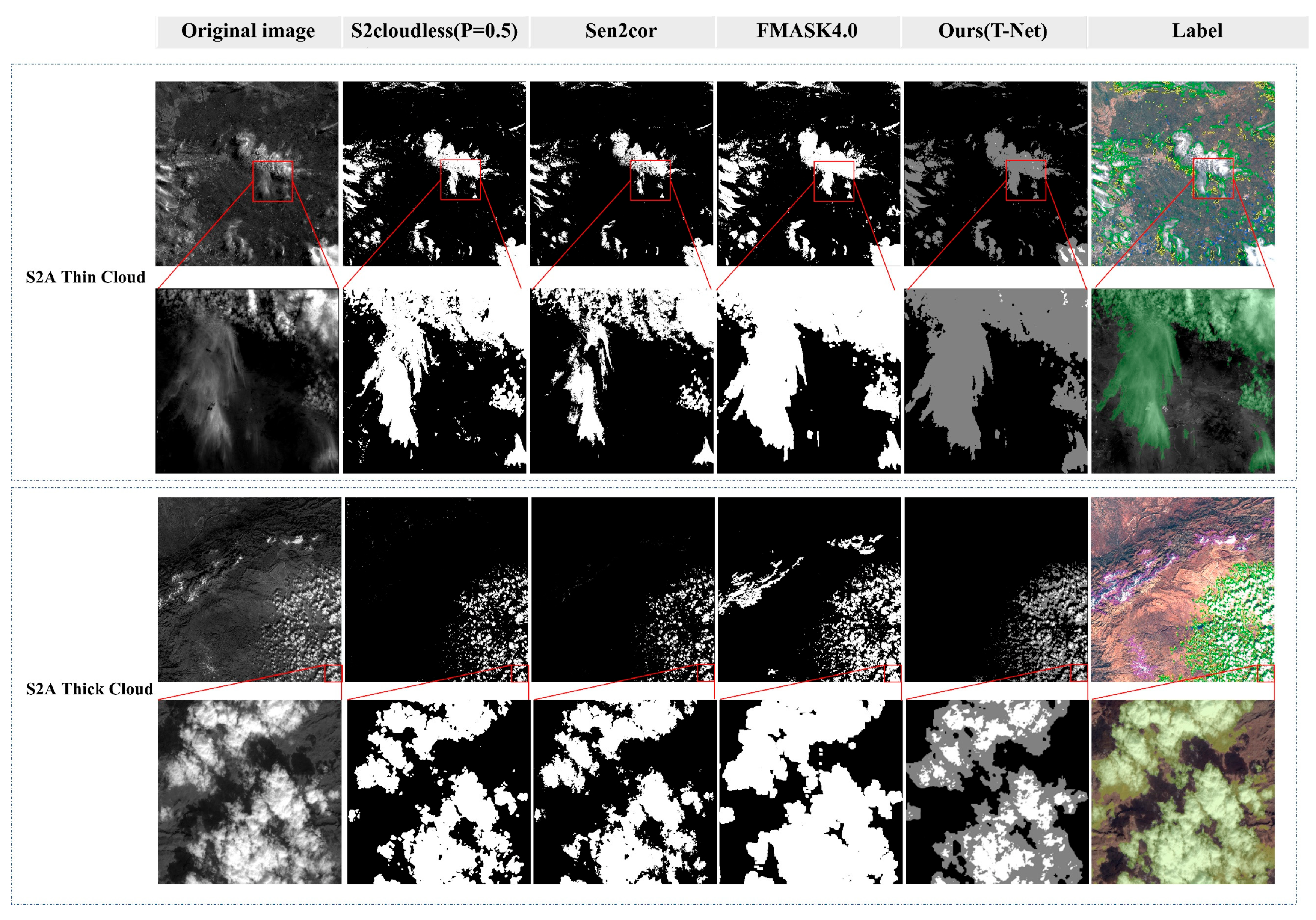
We first validate the cloud detection performance on the ALCD dataset. As shown in Figure 5, S2cloudless (p = 0.5), Sen2cor, FMASK4.0, and T-Net can effectively locate clouds in the Sentinel-2 images. FMASK4.0 and T-Net detection results are more consistent with the actual distribution of thin clouds. Sen2cor and S2cloudless tend to miss some thin cloud features. Although S2cloudless can extract thin clouds better, as the threshold decreases, it will lead to many misclassifications.
S2cloudless (p = 0.5) and Sen2cor extracted more refined results and higher differentiation between clouds and snow in thick cloud regions, whereas FMASK4.0 has a high number of misclassifications due to the lower differentiation between clouds and snow. The T-Net’s results are moderately granular compared to S2cloudless (p = 0.5) and Sen2cor. The T-net model can effectively distinguish thick clouds from thin clouds in trimap because the expansion factor is used in the training process. The T-Net distinguishes clouds and snow better because we build the corresponding bottom map information to enhance the difference between clouds and snow. The misclassification can be effectively reduced in areas where clouds and snow are separated. We calculated five groups of indicators based on thick and thin clouds to compare the cloud detection accuracy of the four models further, and the results are shown in Table 1.
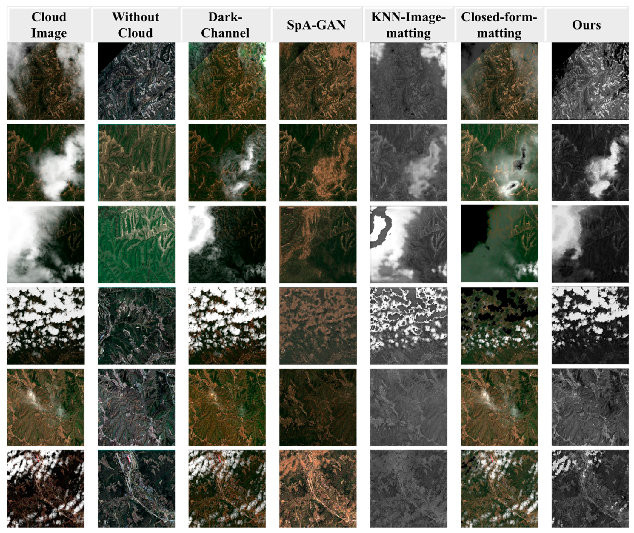
Even if two repeat-pass images are used, obtaining the same surface reflection information is hard. We use a simulated dataset to assess the robustness and accuracy of the cloud removal algorithm. As described in the Introduction section, closed form-matting is similar to our scheme proposed in this paper. Therefore, we emphatically describe the difference from the other three models, such as dark channel, SpA-GAN, and KNN image matting. The cloud removal results are shown in Figure 6. Since most de-clouding models are built using RGB color images, this paper creates a set of corresponding RGB cloud images. The image data types are converted using an alpha superposition operation, resulting in differences in image color parameters in human vision. However, the actual image element’s reflection signals are unaffected.
Dark-channel, closed-form matting, and cloud matting can filter out thin clouds well for image recovery when there are thick or cirrus clouds in the image. In Figure 6, we can see that dark-channel, SpA-GAN, closed-form matting, and cloud matting show a better cloud removal effect when only thin clouds appear in the image. We rank the overall cloud removal effect as our cloud-matting method > SpA-GAN > Dark channel > Closed form mating > KNN image mating. However, it is worth noting the following.
1. When using the dark-channel for remote sensing image de-clouding operations, the estimated projection size is often inversely proportional to the overall brightness of the remote sensing image, resulting in a weakening of feature brightness and a reduction in the overall brightness of the image.
2. Although the SpA-GAN used in this paper performed migration learning on the generated dataset, the results are unsatisfactory. The model’s inference results are close to fitting adjacent image elements. This method is better for de-clouding restoration in thin cloud regions, but in thick cloud regions the model tends to generate image elements with similar characteristics to the entire image, resulting in significant distortions.
3. Both dark-channel and SpA-GAN process the entire image, so regardless of the presence of clouds, both models modify the pixel values of the original image, resulting in pixel distortions in the de-clouded image and making them unsuitable for quantitative, qualitative remote sensing and other studies.
4. KNN image matting and closed-form matting perform de-clouding by estimating the transparency of clouds. However, these methods require a substantial amount of prior manual inputs, such as accurate trimap and maximum reflected brightness of cloud tops. The accuracy of the two models drops significantly or even fails when only thin clouds are in the image. KNN image matting and closed-form matting are limited for cloud removal over remote sensing images.
We observed that the cloud transparency estimation image, i.e., opacity image α , can be obtained using the de-clouded image as the background (Figure 7). Because image α only has brightness variations, and it is no longer disturbed by the image’s background, it can more intuitively reflect the effect of model de-clouding processes. The better the effect of model de-clouding, the closer the brightness variation of the opacity image relative to the label it represents. The degree of damage to the original image during model de-clouding processes is represented by the purity of the opacity image.
According to Equation (2), α = ( ε ε g r o u n d ) / ( ε c l o u d ε g r o u n d ) . Theoretically, the calculated α is greater than 0. The brightness of estimated α from the dark Channel is closest to α ^ , but the background of the α layer is disorderly. Most features are on this layer, resulting in the serious distortion of thick cloud areas. The α obtained by SpA-GAN is less stable, with significant variations in lightness, darkness, and purity, leading to image distortion as well.
KNN image matting is more accurate for α locations. The background of the obtained α is purer than SpA-GAN. The estimation of the transparency probability value has a large offset, making it difficult to recover the image accurately. Closed-form matting estimates the brightness of α , and the purity of α is quite close to the label. However, there will be an underestimation, leading to poor cloud removal effects.
Although there are various methods for single remote sensing image de-clouding, cloud matting can better maintain the original image element information and is less likely to cause image distortion, as shown in the above comparison. We used 640 sets of sliced image pairs to evaluate the restored images in terms of RMSE, SSIM, and PSNR to compare the effect of the five models further. Table 2 shows the results of the evaluation. The SpA-GAN and cloud-matting methods produce the most accurate de-clouding results and cloud transparency. The SpA-GAN metric results are very similar to cloud matting, especially in the mean and minimum values of image de-clouding recovery, which are significantly higher than other methods. However, this is the metric trap of SpA-GAN, which employs a Nash equilibrium-trained model. SpA-GAN uses the model obtained by Nash equilibrium training. Rather than removing the cloud by using the model, the better explanation is that SpA-GAN creates a pixel to minimize the loss function via the generator. Therefore, the model’s accuracy is often high, but the results can be better. As shown in Figure 6 and Figure 7, the result of SpA-GAN in the fourth row of the image is PSNR(Image) = 20.669, while the result of our cloud-matting is PSNR(Image) = 2.820. The image element information in the thick cloud region is completely covered. The thicker the cloud, the lower the reliability of the cloud’s removal result. It is impossible to remove thick clouds by using only one image. The results of SpA-GAN have significant errors, but the overall brightness and structure of the image are very similar to the original one, which lead to large errors. In contrast, cloud-matting results have a higher confidence level. It performs thin cloud removal well in the presence of both thick and thin clouds without damaging the original image.

4. Discussion

Tversky is an efficient and excellent balance loss function for two-class samples. This paper expanded it to multi-class applications. It is suitable for the dataset that we generated and can be effectively applied to other types of negative balance sample research without manual work. Setting the weights can automatically balance the weights of the samples.
Dark channel transmittance estimation has the drawback of not adhering to the imaging mechanism of remote sensing images, causing the image to be enhanced or weakened depending on the brightness of the pixels. The approximate pixels will still be output, resulting in a sharp drop in the model’s reliability.
Generally speaking, GAN added a discriminator based on CNN, which makes the generated image close to the domain of the target image through the Nash equilibrium principle. Therefore, GAN has an additional constraint than CNN. The discriminator calculates the distance between the generated and target image domains, which leads to the fact that the results obtained by GAN on this basis are more in line with human vision. The disadvantage of the methods of CGANs is that the generated data points conform to image distribution characteristics. Furthermore, commonly used single-image cloud removal methods will damage the original remote sensing image’s reflection information, resulting in inconsistent brightness changes in the input and output images.
It is not reasonable to directly apply the SpA-GAN to pin the clouded images to cloudless images. SpA-GAN is an image translation network with an attention mechanism that can be well applied to image restoration tasks. However, if SpA-GAN removes clouds from a single remote sensing image, the obtained cloud removal results must be over-corrected. Since the model learns the mapping from cloudy to cloudless images, it must generate pixels similar to the target domain (cloudless image) in the cloud coverage area. However, clouds in remote sensing images usually cover multiple entities rather than a part of them, which is troublesome for image restoration tasks. Therefore, SpA-GAN and other generated countermeasures networks will output a pixel deception discriminator subject to the target domain. It is challenging to locate these overcorrected pixels, resulting in errors in the cloudless image. Since the characteristics of the cloud are similar to a noise, the discriminator considers the output image true as long as it detects that the generated image conforms to the reasonable noise distribution. However, the generator can easily acquire noise signal and deceive the discriminator. The loss function value provided by the discriminator then is almost meaningless. SpA-GAN degenerates into a CNN network that only relies on the generator and image similarity loss.
In contrast, our cloud-matting model is of great significance for cloud removal. As long as the cloud can be accurately segmented from remote sensing images, cloud removal can be completed without damaging the image surface information. There are many mature methods in the field of cloud detection. The model structure adopted by our method is simple. The model includes only an essential multi-scale image segmentation analysis. Therefore, the accuracy has much room to improve in the future. In the following study, we will perform the following: 1. The model will be improved and trained with the more reliable and advanced backbone. 2. The difficulty of model training and migration will be reduced by combining two-step and one-step methods. 3. The image base maps of heterogeneous areas will be collected to improve the cloud removal results of the model.

5. Conclusions

In this paper, based on the principle of image superposition, we studied the cloud removal of remote sensing images from a new perspective and discussed the principles, advantages, and disadvantages of various single-image cloud removal methods. A set of simulated cloud map generation schemes have been established and is open source. The following conclusions can be drawn from the research findings.
1. The traditional cloud removal models for a single image can only restore the surface information covered by thin clouds. The model’s reliability is significantly reduced when thick and thin clouds coexist.
2. Our cloud-matting scheme only takes the reflection intensity at the top of the cloud into consideration, which is more in line with the imaging mechanism of remote sensing images.
3. Our cloud-matting scheme uses cloud detection to restore surface information based on cloud opacity. It is easily mathematically interpretable, and it does not affect the original cloud-free areas.
4. The experiment results show that our cloud-matting method outperforms other methods. It is worth noting that the GAN image element’s reconstruction ability is powerful in the cloud removal index, but it can easily appear “fabricated” when thick and thin clouds coexist.
5. Using deep learning combined with cloud matting to remove clouds from a single remote sensing image can effectively establish a cloud mask and show good anti-interference performances when thick clouds and thin clouds coexist without damaging the surface information of the original image. Cloud removal with a combination model is a valuable research direction, and we will continue to work in this direction.

Author Contributions

Conceptualization, D.M. and R.W.; methodology, D.M. and R.W.; software, D.M. and R.W.; validation, D.M., R.W. and B.S.; formal analysis, D.M. and R.W.; investigation, D.M. and R.W.; resources, R.W.; data curation, D.M. and R.W.; writing—original draft preparation, D.M. and R.W.; writing—review and editing, D.M. and R.W.; visualization, D.M. and R.W.; supervision, R.W.; project administration, D.M. and D.X.; funding acquisition, D.M. and D.X. All authors have read and agreed to the published version of the manuscript.

Funding

This research was jointly funded by the National Natural Science Foundation of China 491 (Grant No. 51774250) and the Sichuan Science and Technology Program (Grant No. 2022NSFSC1113, 23QYCX0053).

Institutional Review Board Statement

Not applicable.

Informed Consent Statement

Not applicable.

Data Availability Statement

Not applicable.

Conflicts of Interest

The authors declare no conflict of interest.

References

  1. Ju, J.; Roy, D.P. The Availability of Cloud-Free Landsat ETM+ Data over the Conterminous United States and Globally. Remote Sens. Environ. 2008, 112, 1196–1211. [Google Scholar] [CrossRef]
  2. Rossow, W.B.; Schiffer, R.A. Advances in Understanding Clouds from ISCCP. Bull. Am. Meteorol. Soc. 1999, 80, 2261–2287. [Google Scholar] [CrossRef]
  3. Zhang, Y.; Rossow, W.B.; Lacis, A.A.; Oinas, V.; Mishchenko, M.I. Calculation of Radiative Fluxes from the Surface to Top of Atmosphere Based on ISCCP and Other Global Data Sets: Refinements of the Radiative Transfer Model and the Input Data. J. Geophys. Res. Atmos. 2004, D19, 109. [Google Scholar] [CrossRef]
  4. Wu, R.; Liu, G.; Zhang, R.; Wang, X.; Li, Y.; Zhang, B.; Cai, J.; Xiang, W. A Deep Learning Method for Mapping Glacial Lakes from the Combined Use of Synthetic-Aperture Radar and Optical Satellite Images. Remote Sens. 2020, 12, 4020. [Google Scholar] [CrossRef]
  5. Stubenrauch, C.J.C.J.; Rossow, W.B.W.B.; Kinne, S.; Ackerman, S.; Cesana, G.; Chepfer, H.; di Girolamo, L.; Getzewich, B.; Guignard, A.; Heidinger, A.; et al. Assessment of Global Cloud Datasets from Satellites: Project and Database Initiated by the GEWEX Radiation Panel. Bull. Am. Meteorol. Soc. 2013, 94, 1031–1049. [Google Scholar] [CrossRef]
  6. Lin, B.; Rossow, W.B. Precipitation Water Path and Rainfall Rate Estimates over Oceans Using Special Sensor Microwave Imager and International Satellite Cloud Climatology Project Data. J. Geophys. Res. Atmos. 1997, 102, 9359–9374. [Google Scholar] [CrossRef]
  7. Lubin, D.; Harper, D.A. Cloud Radiative Properties over the South Pole from AVHRR Infrared Data. J. Clim. 1996, 9, 3405–3418. [Google Scholar] [CrossRef]
  8. Hahn, C.J.; Warren, S.G.; London, J. The Effect of Moonlight on Observation of Cloud Cover at Night, and Application to Cloud Climatology. J. Clim. 1995, 8, 1429–1446. [Google Scholar] [CrossRef]
  9. Hagolle, O.; Huc, M.; Pascual, D.V.; Dedieu, G. A Multi-Temporal Method for Cloud Detection, Applied to FORMOSAT-2, VENμS, LANDSAT and SENTINEL-2 Images. Remote Sens. Environ. 2010, 114, 1747–1755. [Google Scholar] [CrossRef]
  10. Guosheng, L.; Curry, J.A.; Sheu, R.S. Classification of Clouds over the Western Equatorial Pacific Ocean Using Combined Infrared and Microwave Satellite Data. J. Geophys. Res. 1995, 100, 13811–13826. [Google Scholar] [CrossRef]
  11. Ackerman, S.A.; Holz, R.E.; Frey, R.; Eloranta, E.W.; Maddux, B.C.; McGill, M. Cloud Detection with MODIS. Part II: Validation. J. Atmos. Ocean. Technol. 2008, 25, 1073–1086. [Google Scholar] [CrossRef]
  12. Zhu, Z.; Woodcock, C.E. Object-Based Cloud and Cloud Shadow Detection in Landsat Imagery. Remote Sens. Environ. 2012, 118, 83–94. [Google Scholar] [CrossRef]
  13. Scaramuzza, P.L.; Bouchard, M.A.; Dwyer, J.L. Development of the Landsat Data Continuity Mission Cloud-Cover Assessment Algorithms. IEEE Trans. Geosci. Remote Sens. 2011, 50, 1140–1154. [Google Scholar] [CrossRef]
  14. Zou, Z.; Li, W.; Shi, T.; Shi, Z.; Ye, J. Generative Adversarial Training for Weakly Supervised Cloud Matting. Proceedings of the IEEE Int. Conf. Comput. Vis. 2019, 2019, 201–210. [Google Scholar] [CrossRef]
  15. Foga, S.; Scaramuzza, P.L.; Guo, S.; Zhu, Z.; Dilley, R.D.; Beckmann, T.; Schmidt, G.L.; Dwyer, J.L.; Joseph Hughes, M.; Laue, B. Cloud Detection Algorithm Comparison and Validation for Operational Landsat Data Products. Remote Sens. Environ. 2017, 194, 379–390. [Google Scholar] [CrossRef]
  16. Shi, M.; Xie, F.; Zi, Y.; Yin, J. Cloud Detection of Remote Sensing Images by Deep Learning. In Proceedings of the 2016 IEEE International Geoscience and Remote Sensing Symposium (IGARSS), Beijing, China, 10–15 July 2016; pp. 701–704. [Google Scholar]
  17. le Goff, M.; Tourneret, J.-Y.; Wendt, H.; Ortner, M.; Spigai, M. Deep Learning for Cloud Detection. In Proceedings of the 8th International Conference of Pattern Recognition Systems (ICPRS 2017), Madrid, Spain, 11–13 July 2017; IET: Stevenage, UK, 2017; pp. 1–6. [Google Scholar]
  18. He, Q.; Sun, X.; Yan, Z.; Fu, K. DABNet: Deformable Contextual and Boundary-Weighted Network for Cloud Detection in Remote Sensing Images. IEEE Trans. Geosci. Remote Sens. 2021, 1–16. [Google Scholar] [CrossRef]
  19. Jeppesen, J.H.; Jacobsen, R.H.; Inceoglu, F.; Toftegaard, T.S. A Cloud Detection Algorithm for Satellite Imagery Based on Deep Learning. Remote Sens. Environ. 2019, 229, 247–259. [Google Scholar] [CrossRef]
  20. Mahajan, S.; Fataniya, B. Cloud Detection Methodologies: Variants and Development—A Review. Complex Intell. Syst. 2019, 6, 251–261. [Google Scholar] [CrossRef]
  21. Lin, J.; Huang, T.Z.; Zhao, X.L.; Chen, Y.; Zhang, Q.; Yuan, Q. Robust thick cloud removal for multitemporal remote sensing images using coupled tensor factorization. IEEE Trans. Geosci. Remote Sens. 2022, 60, 1–16. [Google Scholar] [CrossRef]
  22. Pan, X.; Xie, F.; Jiang, Z.; Yin, J. Haze Removal for a Single Remote Sensing Image Based on Deformed Haze Imaging Model. IEEE Signal Process. Lett. 2015, 22, 1806–1810. [Google Scholar] [CrossRef]
  23. Mitchell, O.R.; Delp, E.J.; Chen, P.L. Filtering to Remove Cloud Cover in Satellite Imagery. IEEE Trans. Geosci. Electron. 1977, 15, 137–141. [Google Scholar] [CrossRef]
  24. Li, F.F.; Zuo, H.M.; Jia, Y.H.; Wang, Q.; Qiu, J. Hybrid Cloud Detection Algorithm Based on Intelligent Scene Recognition. J. Atmos. Ocean. Technol. 2022, 39, 837–847. [Google Scholar] [CrossRef]
  25. He, K.M.; SUN, J.T.X.O. Single Image Haze Removal Using Dark Channel Prior. IEEE Trans. Pattern Anal. Mach. Intell. 2011, 33, 2341. [Google Scholar]
  26. Chen, Q.; Li, D.; Tang, C.-K. KNN Matting. IEEE Trans. Pattern Anal. Mach. Intell. 2013, 35, 2175–2188. [Google Scholar] [CrossRef]
  27. Levin, A.; Lischinski, D.; Weiss, Y. A closed-form solution to natural image matting. IEEE Trans. Pattern Anal. Mach. Intell. 2007, 30, 228–242. [Google Scholar] [CrossRef]
  28. Mirza, M.; Osindero, S. Conditional Generative Adversarial Nets. arXiv 2014, arXiv preprint. arXiv:1411.1784. [Google Scholar]
  29. Isola, P.; Zhu, J.-Y.; Zhou, T.; Efros, A.A. Image-to-Image Translation with Conditional Adversarial Networks. In Proceedings of the IEEE Conference on Computer Vision and Pattern Recognition, Hawai, HI, USA, 20–26 June 2017; pp. 5967–5976. [Google Scholar]
  30. Ramjyothi, A.; Goswami, S. Cloud and Fog Removal from Satellite Images Using Generative Adversarial Networks (Gans). 2021. Available online: https://hal.science/hal-03462652 (accessed on 17 November 2022).
  31. Emami, H.; Aliabadi, M.M.; Dong, M.; Chinnam, R.B. Spa-gan: Spatial attention gan for image-to-image translation. IEEE Trans. Multimed. 2020, 23, 391–401. [Google Scholar] [CrossRef]
  32. Wen, X.; Pan, Z.; Hu, Y.; Liu, J. An effective network integrating residual learning and channel attention mechanism for thin cloud removal. IEEE Geosci. Remote Sens. Lett. 2022, 19, 1–5. [Google Scholar] [CrossRef]
  33. Qiu, S.; Zhu, Z.; He, B. Fmask 4.0: Improved Cloud and Cloud Shadow Detection in Landsats 4–8 and Sentinel-2 Imagery. Remote Sens. Environ. 2019, 231, 111205. [Google Scholar] [CrossRef]
  34. Frantz, D.; Haß, E.; Uhl, A.; Stoffels, J.; Hill, J. Improvement of the Fmask Algorithm for Sentinel-2 Images: Separating Clouds from Bright Surfaces Based on Parallax Effects. Remote Sens. Environ. 2018, 215, 471–481. [Google Scholar] [CrossRef]
  35. Housman, I.W.; Chastain, R.A.; Finco, M.V. An Evaluation of Forest Health Insect and Disease Survey Data and Satellite-Based Remote Sensing Forest Change Detection Methods: Case Studies in the United States. Remote Sens. 2018, 10, 1184. [Google Scholar] [CrossRef]
  36. Ji, T.Y.; Chu, D.; Zhao, X.L.; Hong, D. A unified framework of cloud detection and removal based on low-rank and group sparse regularizations for multitemporal multispectral images. IEEE Trans. Geosci. Remote Sens. 2022, 60, 1–15. [Google Scholar] [CrossRef]
  37. Fattal, R. Single image dehazing. ACM Trans. Graph. (TOG) 2008, 27, 1–9. [Google Scholar] [CrossRef]
  38. Sun, Y.; Tang, C.-K.; Tai, Y.-W. Semantic Image Matting. In Proceedings of the IEEE/CVF Conference on Computer Vision and Pattern Recognition, Nashville, TN, USA, 20–25 June 2021; pp. 11120–11129. [Google Scholar]
  39. Chen, Q.; Ge, T.; Xu, Y.; Zhang, Z.; Yang, X.; Gai, K. Semantic Human Matting. In Proceedings of the 2018 ACM Multimedia Conference, Seoul, Republic of Korea, 22–26 October 2018; pp. 618–626. [Google Scholar] [CrossRef]
  40. Xu, N.; Price, B.; Cohen, S.; Huang, T. Deep Image Matting. In Proceedings of the IEEE Conference on Computer Vision and Pattern Recognition, Honolulu, HI, USA, 21–26 July 2017; pp. 2970–2979. [Google Scholar]
  41. Chen, H.; Han, X.; Fan, X.; Lou, X.; Liu, H.; Huang, J.; Yao, J. Rectified cross-entropy and upper transition loss for weakly supervised whole slide image classifier. In International Conference on Medical Image Computing and Computer-Assisted Intervention; Springer: Cham, Switzerland, 2019; pp. 351–359. [Google Scholar]
  42. Salehi, S.S.M.; Erdogmus, D.; Gholipour, A. Tversky Loss Function for Image Segmentation Using 3D Fully Convolutional Deep Networks. In Proceedings of the Lecture Notes in Computer Science (Including Subseries Lecture Notes in Artificial Intelligence and Lecture Notes in Bioinformatics), Quebec City, QC, Canada, 10 September 2017; Springer International Publishing: Berlin/Heidelberg, Germany, 2017; Volume 10541, pp. 379–387. [Google Scholar]
  43. Lin, T.-Y.; Goyal, P.; Girshick, R.; He, K.; Dollar, P. Focal Loss for Dense Object Detection. In Proceedings of the IEEE International Conference on Computer Vision, Venice, Italy, 22–29 October 2017; Volume 2017, pp. 2999–3007. [Google Scholar]
  44. Li, X.; Sun, X.; Meng, Y.; Liang, J.; Wu, F.; Li, J. Dice Loss for Data-Imbalanced NLP Tasks. arXiv 2020, arXiv:1911.02855. [Google Scholar]
  45. Wang, L.; Wang, C.; Sun, Z.; Chen, S. An Improved Dice Loss for Pneumothorax Segmentation by Mining the Information of Negative Areas. IEEE Access 2020, 8, 167939–167949. [Google Scholar] [CrossRef]
  46. Rhemann, C.; Rother, C.; Wang, J.; Gelautz, M.; Kohli, P.; Rott, P. A Perceptually Motivated Online Benchmark for Image Matting. In Proceedings of the 2009 IEEE Conference on Computer Vision and Pattern Recognition, CVPR, Miami, FL, USA, 20–25 June 2009; pp. 1826–1833. [Google Scholar]
  47. Shen, X.; Tao, X.; Gao, H.; Zhou, C.; Jia, J. Deep Automatic Portrait Matting. In Proceedings of the Computer Vision–ECCV 2016: 14th European Conference, Amsterdam, The Netherlands, 11–14 October 2016; Springer International Publishing: Berlin/Heidelberg, Germany, 2016; Volume 9905, ISBN 9783319464473. [Google Scholar]
  48. Irish, R.R.; Barker, J.L.; Goward, S.N.; Arvidson, T. Characterization of the Landsat-7 ETM+ Automated Cloud-Cover Assessment (ACCA) Algorithm. Photogramm. Eng. Remote Sens. 2006, 72, 1179–1188. [Google Scholar] [CrossRef]
  49. Hughes, M.J.; Hayes, D.J. Automated Detection of Cloud and Cloud Shadow in Single-Date Landsat Imagery Using Neural Networks and Spatial Post-Processing. Remote Sens. 2014, 6, 4907–4926. [Google Scholar] [CrossRef]
  50. Baetens, L.; Desjardins, C.; Hagolle, O. Validation of Copernicus Sentinel-2 Cloud Masks Obtained from MAJA, Sen2Cor, and FMask Processors Using Reference Cloud Masks Generated with a Supervised Active Learning Procedure. Remote Sens. 2019, 11, 433. [Google Scholar] [CrossRef] [Green Version]
  51. Louis, J.; Debaecker, V.; Pflug, B.; Main-Knorn, M.; Bieniarz, J.; Mueller-Wilm, U.; Cadau, E.; Gascon, F. Sentinel-2 SEN2COR: L2A Processor for Users. In Proceedings of the Living Planet Symposium 2016, Spacebooks Online, Prague, Czech Republic, 9–13 May 2016; Volume SP-740, pp. 1–8, ISBN 978-92-9221-305-3. [Google Scholar]
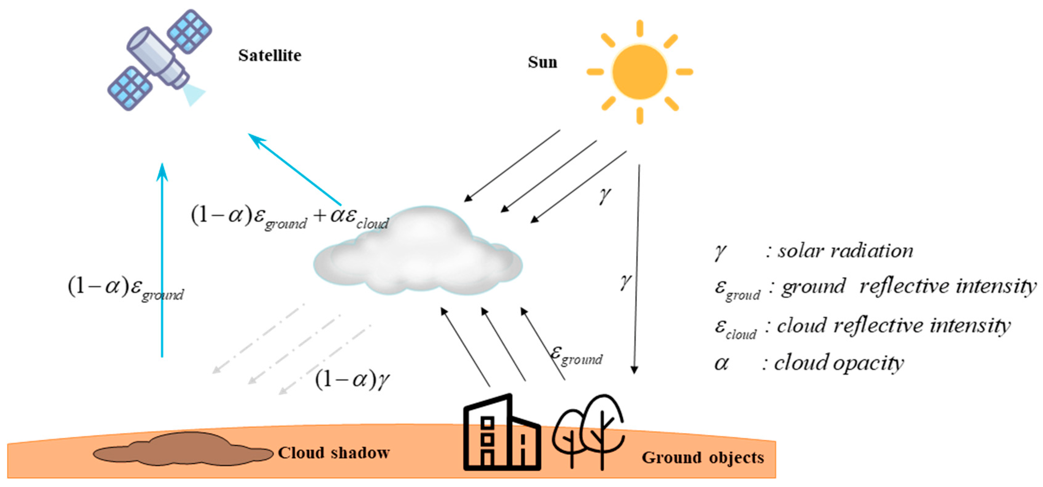
Figure 1. A schematic diagram of the remote sensing imaging process. The reflected energy received by sensors is a linear superposition of the reflected energy from the cloud’s top and the reflected energy from the surface for given cloud transparency.
Remotesensing 15 00904 g001
Figure 2. Two-step cloud-matting model.
Remotesensing 15 00904 g002
Figure 3. Cloud-matting dataset generation. Columns 1–3: The cloud-free image base map with Sentinel-2 Band2. The cloud transparency information notation is α . The cloud shadow notation is f ( 1 α ) , which is randomly generated according to cloud transparency, and f represents the offset calculation. The fourth column is the trimap image of the cloud, and we set α > 0.9 relative to the cloud-trimap foreground. The fifth column is the composite image with clouds.
Remotesensing 15 00904 g003
Figure 4. Confusion matrix applied to the evaluation index.
Remotesensing 15 00904 g004
Figure 5. Cloud detection comparison experiments. The first to sixth columns are Band-2 image information, S2cloudless cloud detection results with a probability greater than 0.5, Sen2cor-2.09 cloud detection results, FMASK4.0 cloud detection results, T-Net trisection prediction results, and ALCD Tags.
Remotesensing 15 00904 g005
Figure 6. Comparison of cloud removal results of five models. The first to seventh columns are remote sensing images with clouds, remote sensing images without clouds, dark-channel, SpA-GAN, KNN image matting, closed-form matting, and our proposed cloud-matting method, respectively.
Remotesensing 15 00904 g006
Figure 7. Comparison of estimated cloud transparency images.
Remotesensing 15 00904 g007
Table 1. Comparison of the accuracy of four cloud detection methods.
MethodsSen2corS2cloudlessFmask4.0Ours-TNetLabel
Precision (thin cloud)0.68370.77120.77620.7981
Recall (thin cloud)0.96320.94000.92710.9445
Accuracy (thin cloud)0.94580.95600.95500.9596
IoU (thin cloud)0.66630.73510.73150.7551
Cloud content (thin cloud)9.474012.97517.27116.31515.815
Precision (thick cloud)0.66580.71720.76990.8019
Recall (thick cloud)0.88350.87570.86430.8665
Accuracy (thick cloud)0.94090.94480.94770.9596
IoU (thick cloud)0.61220.65090.68680.7254
Cloud content (thick cloud)4.49605.700013.40010.81012.190
Table 2. Comparison of five cloud removal methods. The optimal value, average value, and worst value of the cloud removal result are represented by green, blue, and red, respectively.
MetricsDark-ChannelSpA-GANKNN Image MattingClosed-Form MattingOurs
RMSE (Image)0.02330.01210.00730.00650.0025
0.12340.10980.86200.14290.2121
0.33960.37887.16331.14193.2967
SSIM (Image)0.81980.99590.99220.99420.9992
0.41150.83210.61530.74180.8120
0.15420.25700.02760.14040.1040
PSNR (Image)32.629644.172342.693943.687151.8999
19.339426.770411.134420.063223.8369
9.37978.4318−17.1023−1.1526−10.3616
RMSE (Alpha)0.00590.00710.01290.01590.0067
0.08030.03140.23820.11410.0263
0.29930.07930.82590.60570.0791
SSIM (Alpha)0.99280.99410.98930.99530.9967
0.81710.86160.75370.85880.9810
0.49600.64120.00000.42680.9350
PSNR (Alpha)44.560243.115137.787235.933843.3984
23.800930.517217.036521.199332.7192
10.476823.17981.66134.354022.0270
Disclaimer/Publisher’s Note: The statements, opinions and data contained in all publications are solely those of the individual author(s) and contributor(s) and not of MDPI and/or the editor(s). MDPI and/or the editor(s) disclaim responsibility for any injury to people or property resulting from any ideas, methods, instructions or products referred to in the content.