An Enhanced Residual Feature Fusion Network Integrated with a Terrain Weight Module for Digital Elevation Model Super-Resolution

Abstract

The scale of digital elevation models (DEMs) is vital for terrain analysis, surface simulation, and other geographic applications. Compared to traditional super-resolution (SR) methods, deep convolutional neural networks (CNNs) have shown great success in DEM SR. However, in terms of these CNN-based SR methods, the features extracted by the stackable residual modules cannot be fully utilized as the depth of the network increases. Therefore, our study proposes an enhanced residual feature fusion network (ERFFN) for DEM SR. The designed residual fusion module groups four residual modules to make better use of the local residual features. Meanwhile, the residual structure is refined by inserting a lightweight enhanced spatial residual attention module into each basic residual block to further strengthen the efficiency of the network. Considering the continuity of terrain features, terrain weight modules are integrated into the loss module. Based on two large-scale datasets, our ERFFN shows a 10–20% reduction in the mean absolute error and the lowest error in terrain features, such as slope, demonstrating the superiority of an ERFFN-based DEM SR over state-of-the-art methods. Finally, to demonstrate potential value in real-world applications, we deploy the ERFFN to reconstruct a large geographic area covering 44,000 km² which contains missing parts.

1. Introduction

As a digital representation of the regional terrain surface, the digital elevation model (DEM) is inherently multi-scale in nature, and various geological analyses and simulations based on DEMs are also highly scale-dependent [1,2]. However, the prevailing multiscale DEM data suffer from scale fragmentation, scale discontinuity, data redundancy, and other challenges, which are unable to meet the demand of multiscale terrain analysis [3,4]. 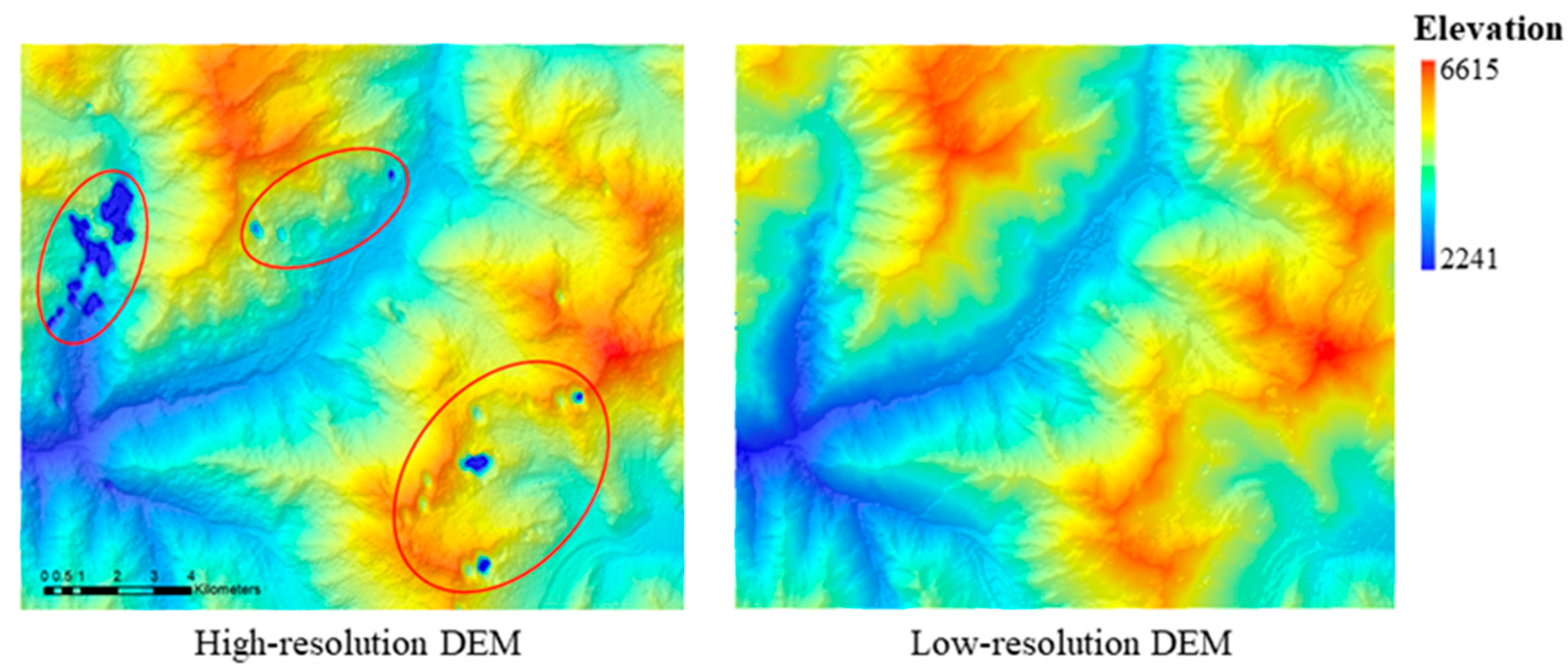Recently, high-resolution DEMs have been obtained from costly high-precision sensors [5] and other dense image-matching techniques to generate high-resolution DEMs [6], but methods for generating higher-resolution DEMs from low-resolution DEMs without extra sensors and cameras are rarely discussed. Furthermore, when part of the high-resolution DEM data is missing or only a small region of data with similar topography can be obtained, as Figure 1 demonstrates, effectively enhancing the resolution of DEMs and improving the quality of DEM data to reconstruct large-scale DEMs based on existing data may yield new benefits [7,8,9].

DEM super-resolution (SR) represents restoring the scale of DEM data from low-resolution DEM data [10]. The main SR methods based on DEM data can be divided into learning-based methods, traditional approaches that contain interpolation-based methods [11,12], and data fusion-based methods [13,14,15]. Traditional interpolation methods, such as inverse distance weighted (IDW), kriging, and bilinear interpolation, are the most widely used approaches because of their speed and simplicity, but the generated DEMs may suffer smoothing issues due to the lack of exploitation of non-local information about disjoint regions when applied to large-scale DEM reconstruction. The data fusion-based methods are applied to fill gaps between a variety of data sources and obtain high-quality DEMs with the constraint of many hyper-parameters. However, the inefficiency and low accuracy of the traditional methods make them inferior to deep-learning methods, which can reconstruct large-scale DEM data after being trained using several small areas of the region with similar topography.

Nowadays, in the SR domain, most of the approaches are aimed at natural pictures in computer vision (CV) [16,17,18,19] and remote sensing images [20,21]. The super resolution convolutional neural network (SRCNN) [16] was the first end-to-end SR algorithm and provided better performance when compared to more conventional approaches. Motivated by pioneering work, the deeper Very Deep Convolutional Networks (VDSR) [22] and Deeply-Recursive Convolutional Network (DRCN) [23] with 20 layers were designed based on residual learning. However, the interpolated feature maps are computationally intensive and consume a lot of memory, leading to the deconvolutional layer in FSRCNN [24] and the sub-pixel layer in the efficient sub-pixel CNN [25] inserted at the end of the architecture to make a more lightweight SR network. Moreover, removing the batch normalization layer in the enhanced deep residual network (EDSR) [17] further reduced the parameters of the network, resulting in better performance of a network containing the same parameters. Therefore, the total number and the complexity of the stackable modules can be improved to obtain more representations [19]. Retrieved from attention mechanisms widely used in the CV domain [26,27,28,29], and residual structures that exert an enormous influence on feature aggregation [18], some attention-based modules have been integrated with a residual block to further improve the SR network performance. The residual channel attention module in the residual channel attention network (RCAN) [30], the channel-wise and spatial feature module in the channel-wise and spatial feature modulation network (CSFM) [31], the second-order attention module in the second-order attention network (SAN) [32], and the enhanced spatial attention module in the residual feature aggregation network (RFAN) [18] can all obtain more powerful feature representation than the ordinary residual block.

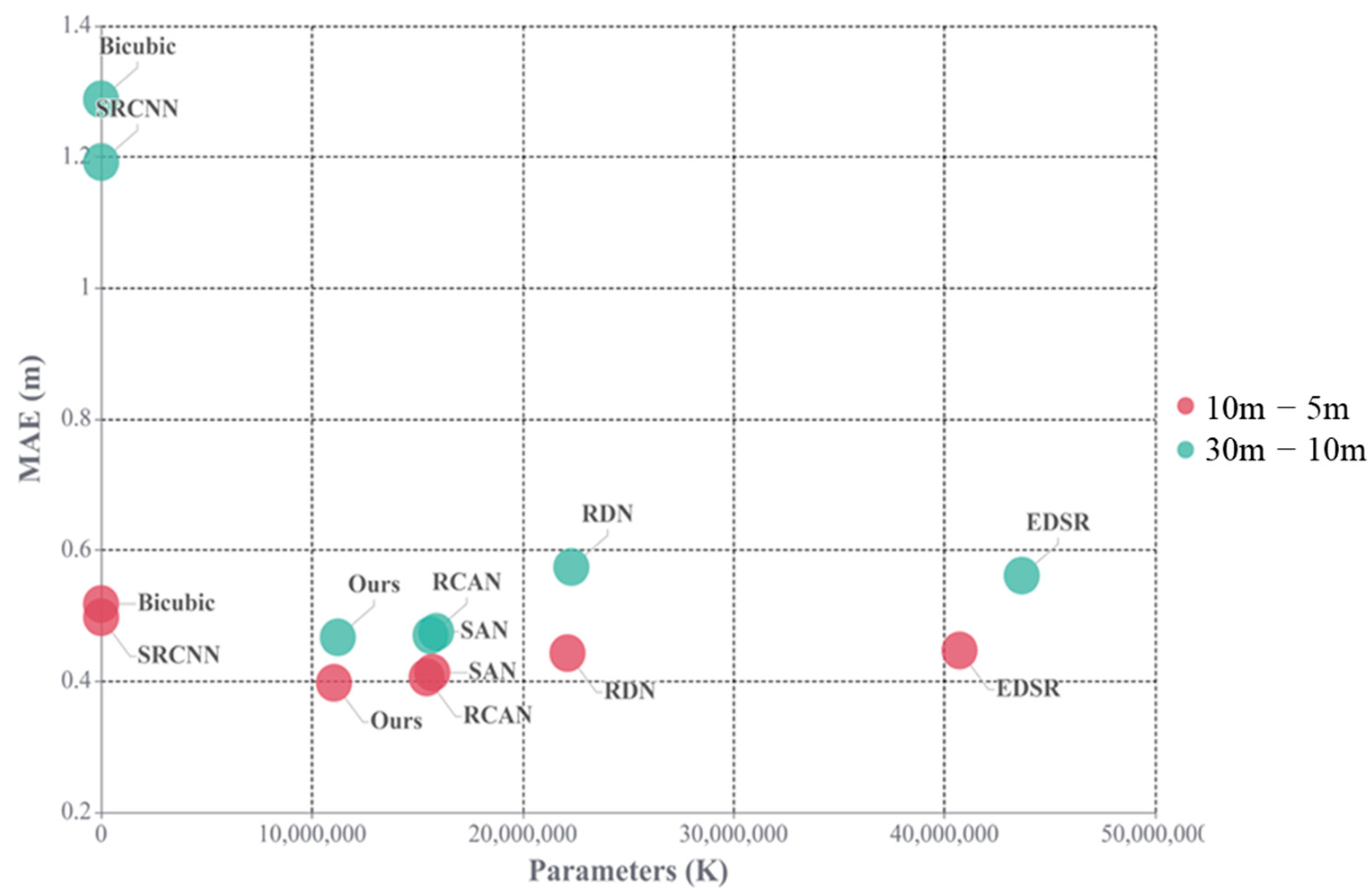
Although significant improvements have been made in single-image SR (SISR), existing state-of-the-art learning-based models suffer from several constraints. Generally, a network for SR contains a series of stackable residual modules to enhance the feature representation extraction, such that a shallow feature can only exert a main influence on the next module, and the shallow feature has a lengthy path to exert influence on the ultimate feature. With the increase in the complexity and depth of the network, the features in the stackable modules will be layered with different perceptual fields and cannot be taken full advantage of in the representation of the intermediate layers of most of the existing learning-based models.

Moreover, these natural and remote sensing images are different from single-band DEMs, so typical SR techniques cannot be directly applied to DEM data [33,34], the main purpose of which is to obtain accurate elevation values. As for the learning-based algorithms, the CNN was first transferred from image SR to single-band DEM SR in 2016 [10]. Subsequently, innovations have gradually led to improved outcomes in the DEM SR domain. Ref. [8] enhanced the EDSR model by integrating gradient prior knowledge and transfer learning, which achieved excellent performance. Considering the current single scale in DEM SR, Ref. [33] designed a multiscale DEM reconstruction architecture to generate high-resolution DEMs using multiscale supervision. Moreover, taking a mountain area into account, Ref. [35] combined the residual block and VDSR to reconstruct the DEM with obvious undulation characteristics. Ref. [36] refined the ESPCN and proposed the Recursive Sub-pixel Convolutional Neural Network (RSPCN) to generate finer-scale DEMs from low-resolution DEMs. In addition, other visual quality-oriented methods represented by generative adversarial networks (GANs) have also been developed in the DEM SR field. A conditional encoder–decoder generative adversarial network (CEDGAN) [37] was proposed to combine the encoder–decoder structure with adversarial learning for spatial interpolation. Then, the topographical features were gradually combined with DEM SR networks. Ref. [34] designed a loss function integrating the qualitative topographic knowledge of valley lines and ridge lines to complete the generation of gap DEMs. Explicit terrain feature-aware optimization was integrated into the loss module of the network [9]. However, topographic specificity and consistent maintenance of terrain features both need to be considered sufficiently.

Moreover, in terms of the current different scales of DEMs, the degradation model and the blurred kernel are often unknown, and the low-resolution DEMs are not simply obtained using interpolation-based methods from the high-resolution DEMs. Therefore, the network trained with paired data generated using interpolation-based methods only simply fits the inverse process of interpolation, which lacks practical significance in the real world. However, the significance of taking real-world low-resolution DEM datasets as training datasets instead of data obtained using downsampling from high-resolution data has been overlooked thus far [38].

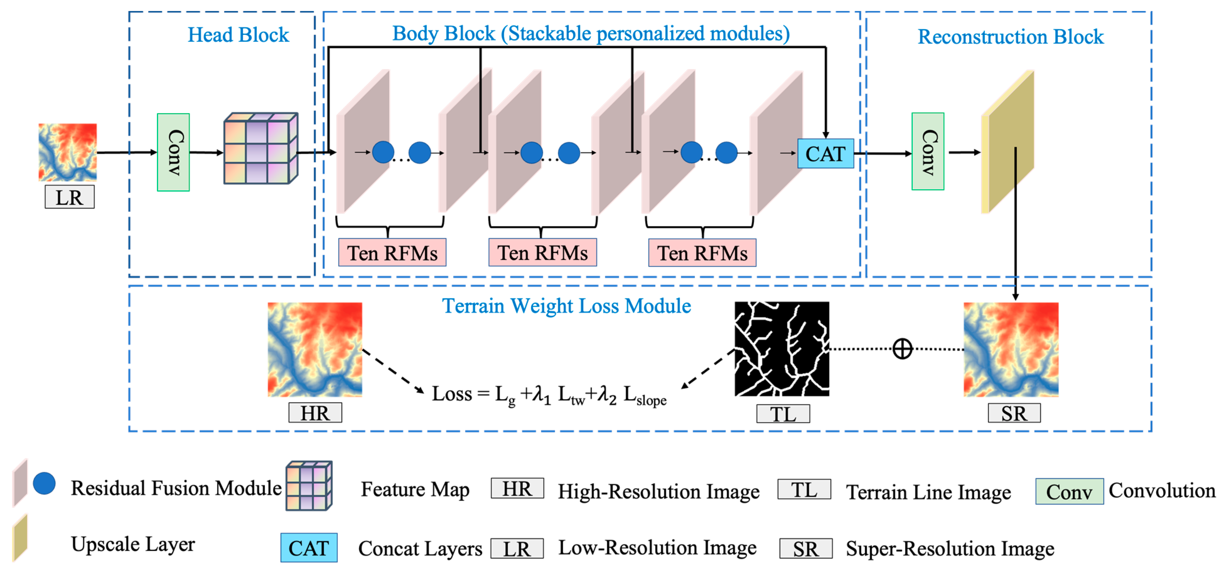
Therefore, in this paper, an enhanced residual feature fusion network (ERFFN), is designed to address the three issues depicted above: the lack of the exploitation of residual features, insufficient integration of terrain features, and the lack of practical significance of application scenarios. The ERFFN achieves superior results compared to the other state-of-the-art SR methods for DEM imagery. The main contributions of our study are summarized as follows:

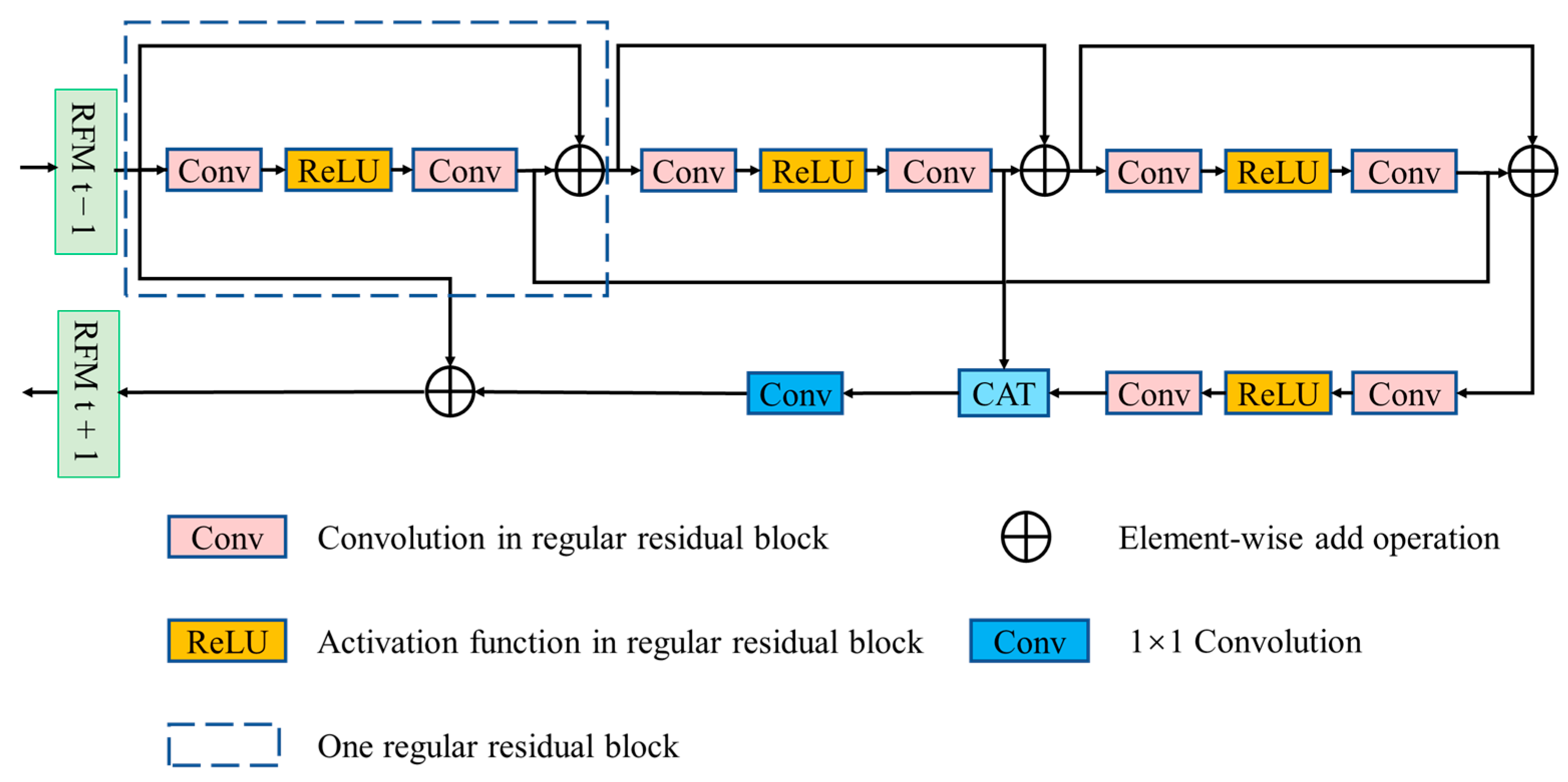
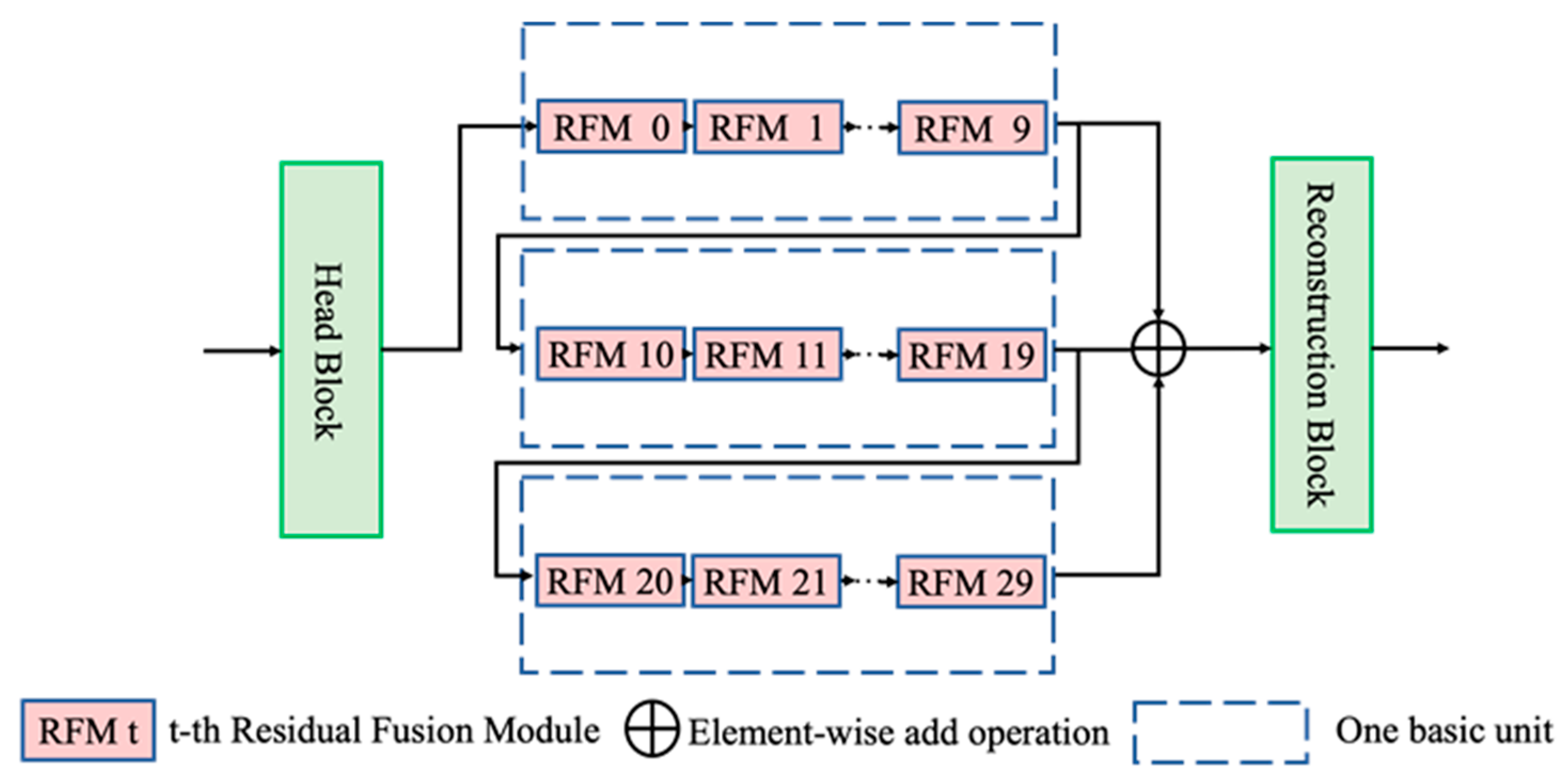
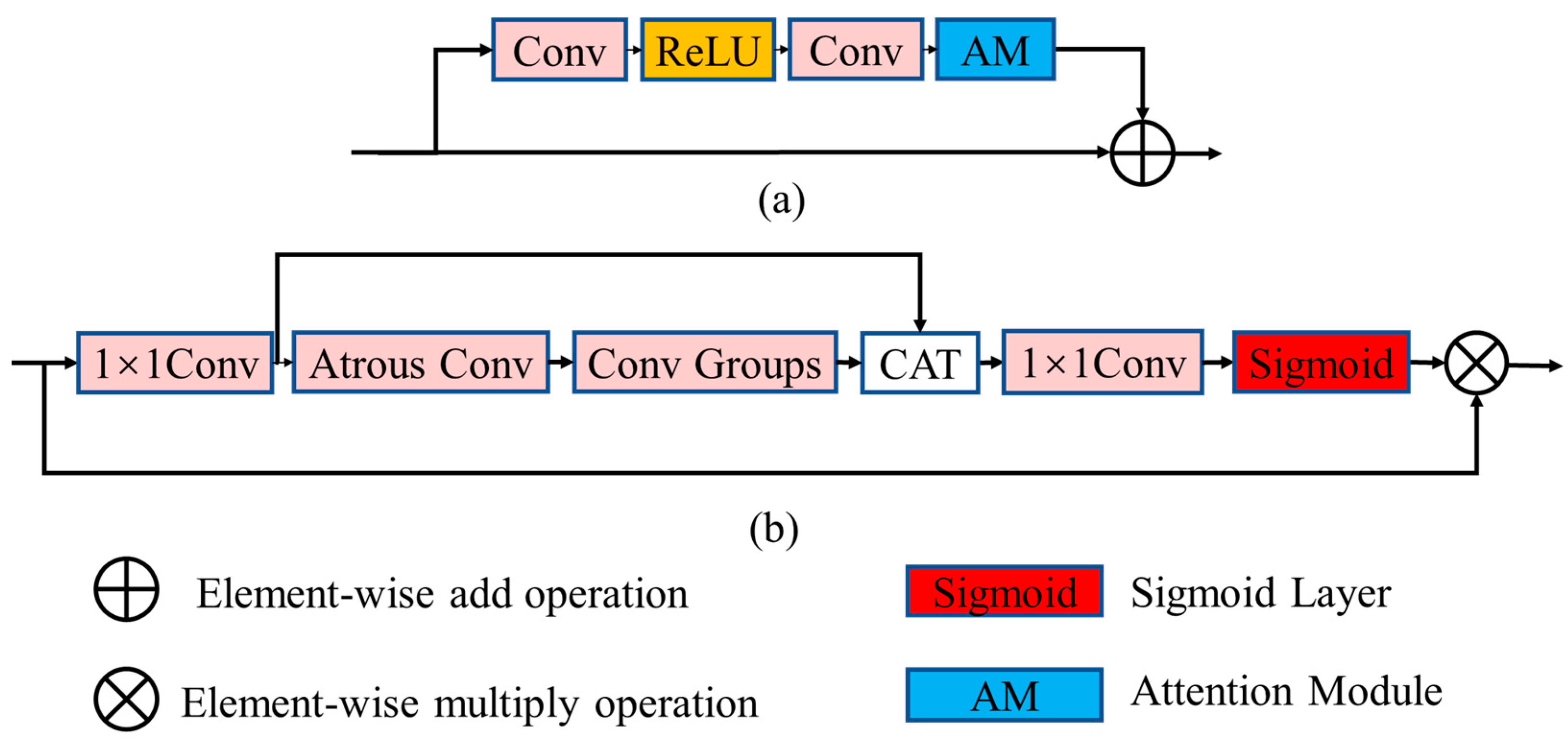
• To enhance the utilization of residual features, a residual fusion module (RFM) is proposed for DEM SR. Our approach can propagate the influence of the intermediate features at a fraction of the cost, thus leading to effective feature extraction with a strong representation from DEM images and achieving a better trade-off between efficiency and performance.
• Considering the relevance of residual features in the exploitation of feature representation, we refine the residual structure by inserting a lightweight enhanced spatial residual attention module (ESRAM) into each basic residual block to further strengthen the reconstruction accuracy of our proposed network.
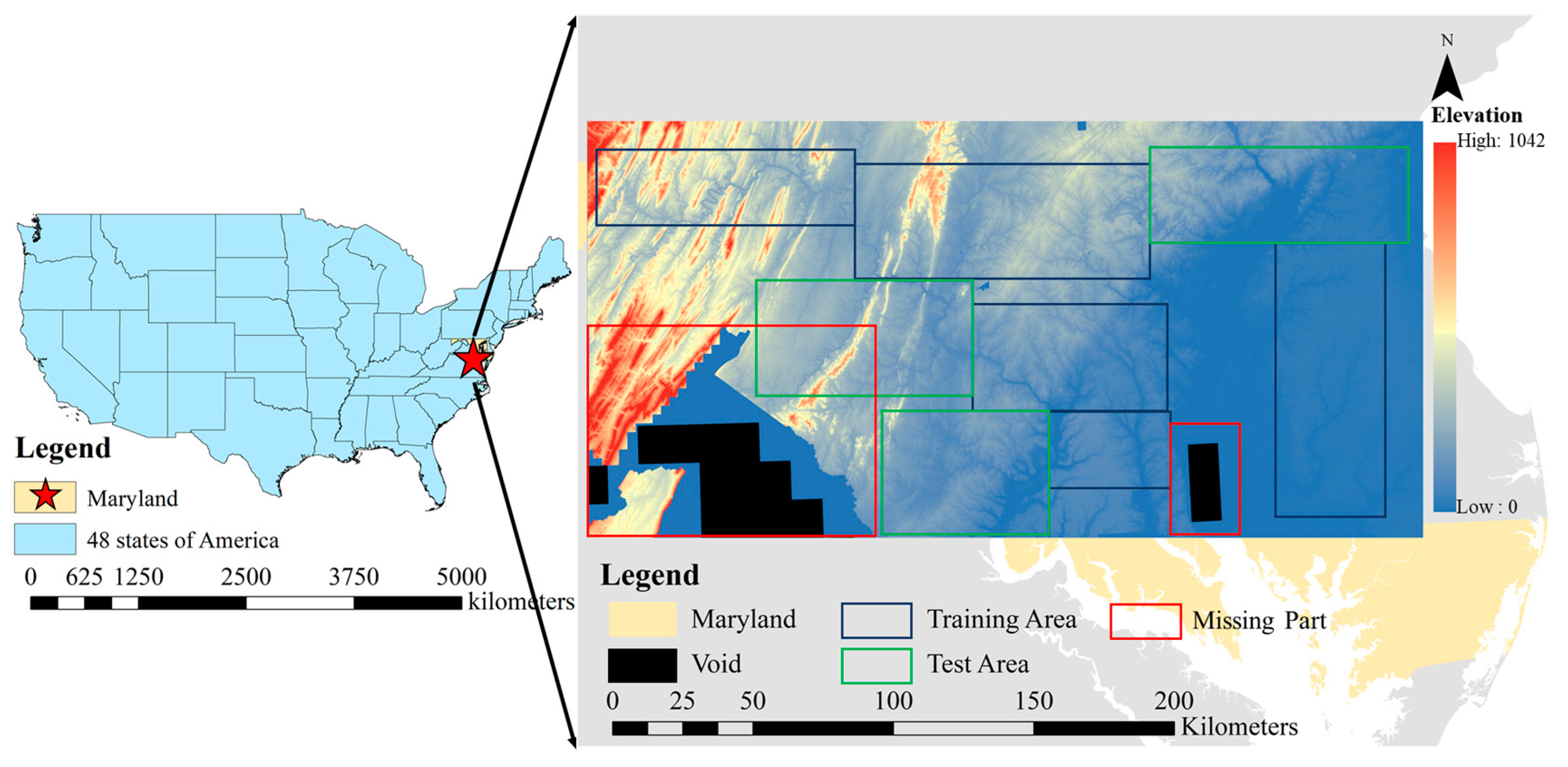
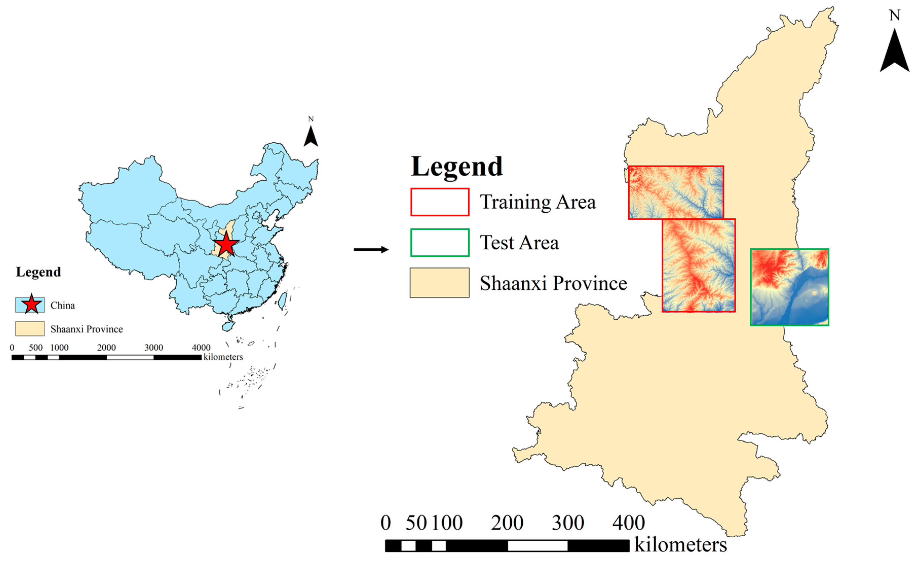
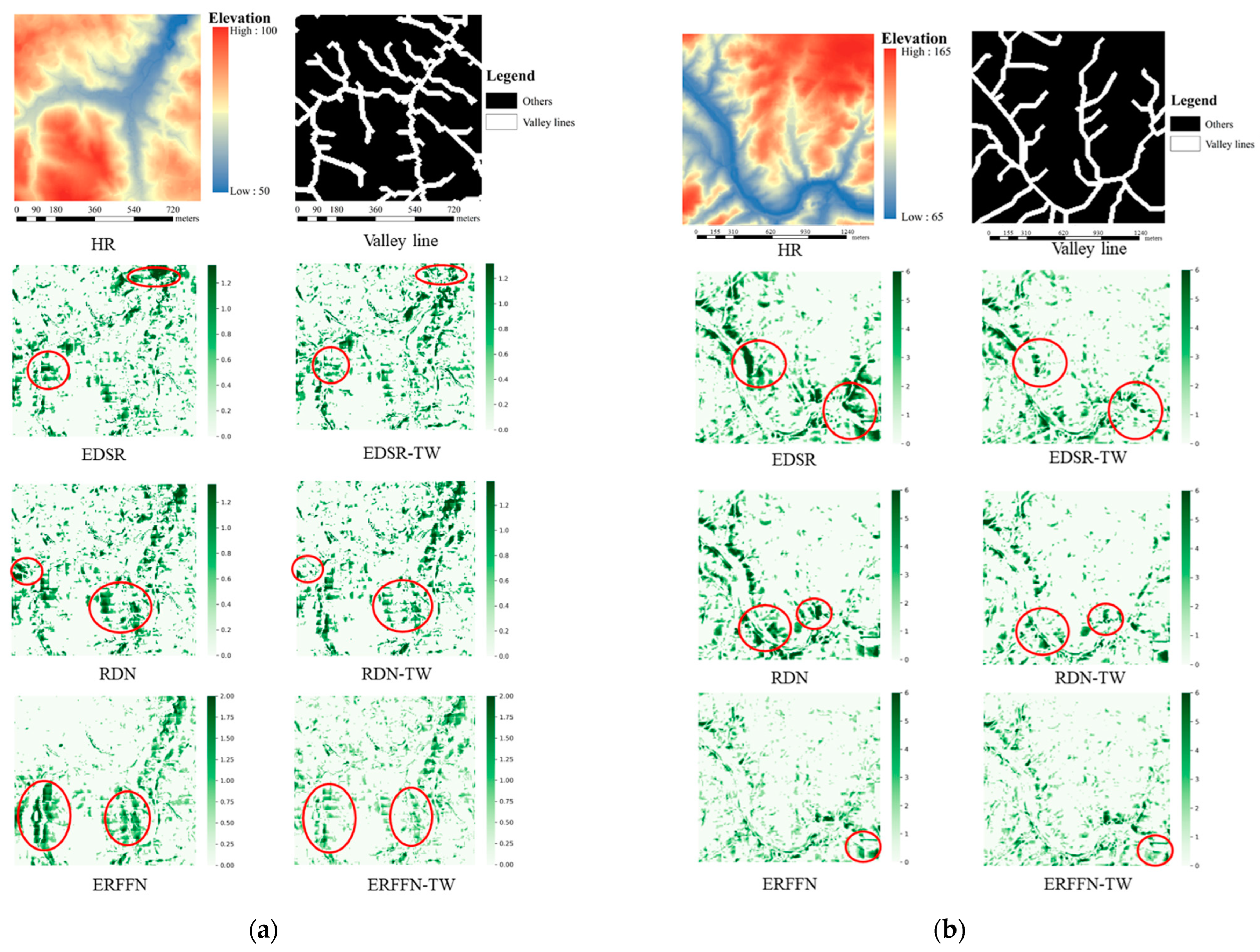
• To sufficiently maintain continuity of the terrain features, a terrain weight loss module that incorporates slope loss and terrain feature loss is designed to learn strongly discriminative and topographic feature representations. Simultaneously, the proposed method is trained and evaluated using two large-scale DEM datasets for different reconstruction scales, and we deploy the trained model to reconstruct a missing part of the current high-resolution DEMs, which improves practical significance.

The remainder of this paper is organized as follows. Section 2 presents the proposed architecture based on DEM data and the implementation details. The experimental data and training details are presented in Section 3. The results are discussed in Section 4 and finally, some conclusions are presented in Section 5.

2. Methodology

To address the issues raised above, we propose an ERFFN to make better use of the intermediate residual features for a more efficient and robust DEM SR. The overall framework is illustrated in Figure 2. The ERFFN consists of a head block for elementary feature extraction, a body block containing stackable RFMs, and a reconstruction block, which is trained by optimizing a terrain weight loss module. Our designed ESRAM is a part of the RFM in the body block, which is not identified in Figure 2 and is discussed in more detail below.

2.1. Residual Feature Fusion Module

The latest SR networks tend to have similar components. As shown in some state-of-the-art methods for image SR, a basic network generally consists of head, body, and reconstruction blocks. The head block, composed of only one convolution layer and one active layer, is designed to convert the initial pixel values in the original image into an elementary feature ($F_0)$ as the input of the body block responsible for hierarchical feature extraction with a series of stackable personalized modules (PMs), such as the residual modules in EDSR [17]. The body block can be formulated as:

$$F_t={{\rm P}}_t\left(F_{t-1}\right)={{\rm P}}_t({{\rm P}}_{t-1}\left(\cdots {{\rm P}}_0\left(F_0\right)\cdots \right)$$

(1)

where ${{\rm P}}_t$ represents the $t$-th personalized modules and $F_{t-1}$ and $F_t$ are the input and the output feature map of the $t$-th PM function, respectively. $F_0$ is operated with a long skip connection to make an element-wise addition to $F_t$ as the input feature of the reconstruction block, which can be formulated as:

$$SR=\mathcal{R}\left(F_0+F_t\right)$$

(2)

where $SR$ is the output of the entire network and $\mathcal{R}$represents the reconstruction function, which consists of upscale modules, such as a sub-pixel convolutional layer and a deconvolutional layer.

Throughout the pipeline of the regular image SR mentioned above, the stackable PM accounts for most of the feature aggregation. However, as shown in Equations (1) and (2), the long skip connection only exists in the input of the reconstruction part, resulting in the shallow feature having to go through a lengthy path to exert an influence on the ultimate feature. Consequently, we design an RFM as the PM of our paper to make better use of the local residual features and build an effective network for the DEM SR, as depicted in Figure 3.

Every RFM contains four residual blocks, wherein every residual block consisting of two 3 × 3 convolutional layers and one activation function can obtain a local feature. The residual features from the first three residual blocks are concatenated together with the output of the last residual block as the input of a 1 × 1 convolutional layer to fuse the residual features and reduce the spatial dimension before an element-wise addition to the low-level feature extracted from the previous RFM. Compared to simple multiple stackable residual blocks, the RFM can propagate the influence of the intermediate features at a fraction of the cost, thus leading to effective feature extraction with a strong representation from DEM images. Different from briefly stacking thirty residual feature aggregation modules derived using the RFAN [18], our framework also takes the fusion of the local feature extracted from each RFM into account, which considers every ten RFMs as one basic unit having the same role as one residual block in the RFM and can be referred to as an “aggregation of the residual features after fusion”. The overall body block is illustrated in Figure 4.

The proposed RFM is a general architecture that can be easily applied to the existing SR blocks for DEM SR construction.

2.2. Enhanced Spatial Residual Attention Module

As mentioned above, the attention structure significantly affects the feature aggregation, prompting us to propose an enhanced residual module to maximize the effectiveness of our RFM for DEM SR. Therefore, an enhanced spatial residual attention module (ESRAM) is proposed that works at the end of the residual module in our method to enhance the performance of the designed RFM, as depicted in Figure 5a, and exhibits more reasonable and powerful performance than the channel attention (CA) module in the RCAN [30], which is depicted in Figure 5b.

The reduction in the channel dimension is achieved by the first 1 × 1 convolutional layer of the proposed ESRAM. Then, we design a dilated convolutional layer to enlarge the receptive field of the block without changing the spatial dimension. Atrous convolution is widely used in the CV domain to obtain receptive field enlargement; therefore, we set the dilated parameter of the convolutional layer as six. The reason why we do not enlarge the receptive field by setting a larger dilated parameter (such as 12) is that the additional 0-value padding added to the edges of the DEM image accounts for most of the feature maps used for convolution and leads to a weak representation for DEM images. Then, the groups consisting of three 3 × 3 convolutional layers reorganize the feature representation, and a skip connection is utilized to forward the low-level features and concentrate the features as the input to one 1 × 1 convolutional layer to recover the channel dimensions. Last but not least, a sigmoid layer is designed to generate an element-wise attention factor that is multiplied by the residual feature extracted from the previously connected residual block.

2.3. Terrain Weight Loss Function

Generally, there exist special terrain features in DEMs, which regular SR networks do not consider. Inspired by the concept of slope loss combined with its loss functions for DEM SR [9], our method also takes slope loss into account as the key part of our loss module. Meanwhile, the prediction results of ordinary SR networks reveal that the predicted elevation errors are larger in areas with large topographic relief, such as the neighborhoods of valley lines, compared to flat areas. Therefore, it is necessary to set different weights for areas with large terrain undulations and flat areas to train a model. In summary, the entire loss function is formulated as follows:

$$\mathcal{L}={\mathcal{L}}_{global }+ {\lambda }_1{\mathcal{L}}_{slope}+{\lambda }_2{\mathcal{L}}_{tw}$$

(3)

where ${\mathcal{L}}_{global}$, ${\mathcal{L}}_{slope}$, and ${\mathcal{L}}_{tw}$ represent global loss, slope loss, terrain-weighted loss, respectively, which are described in detail below. The weights of ${\mathcal{L}}_{slope}$ and ${\mathcal{L}}_{tw}$ (${\lambda }_1$ and ${\lambda }_2$) depend on the scale factor of SR.

(1)

Global loss.

The global loss is calculated as follows:

$${\mathcal{L}}_{global}= \frac{1}{\mathsf{{\rm N}}}{\displaystyle \sum }_i^N\left|h_i-{\widehat{h}}_i\right|$$

(4)

where N represents the total number of pixels in a DEM image, $h_i$ represents the true elevation value of the $i$-th DEM cell, and ${\widehat{h}}_i$ denotes its elevation value after SR.

(2)

Slope loss.

The slope of every DEM cell except the edges is calculated as follows:

$$d{x}_i=\frac{\left(h_{i+1}-h_{i-1}\right)}{2s}$$

(5)

$$d{y}_j=\frac{\left(h_{j+1}-h_{j-1}\right)}{2s}$$

(6)

$$slop{e}_{ij}=\arctan \sqrt{d{x}_i{}^2+d{y}_j{}^2+eps}$$

(7)

where $d{x}_i$ and $d{y}_i$ represent the $i$-th gradient in the $x$-direction and the $j$-th gradient in the $y$-direction, respectively, s devotes the resolution of the DEM, and $eps$ is applied to let the gradient be non-zero when performing backpropagation, which is set to 10⁻⁸ in this paper.

The slope loss is then calculated as:

$${\mathcal{L}}_{slope}= \frac{1}{{\rm N}}{\displaystyle \sum }_i^N\left|S_i-{\widehat{S}}_i\right|$$

(8)

where $S_i$ represents the slope value of the $i$-th DEM cell, and ${\widehat{S}}_i$ denotes its slope value after SR.

(3)

Terrain-weighted loss.

As terrain features enhance the effect of DEM SR reconstruction, we take near-valley lines into account. When calculating the loss values, the pixels of the near-valley lines are used to mark the valley lines, thus highlighting the supervised learning of the valley lines, which is given by:

$${\mathcal{L}}_{tw}= \frac{1}{M}{\displaystyle \sum }_i^M\left|h_i\times C_i-{\widehat{h}}_i\times C_i\right|$$

(9)

where M represents the number of pixels of near-valley lines in a DEM image, and $C_i$ represents the category value of the $i$-th DEM cell with possible values of 0 for flat areas or 1 for areas with large topographic relief.

3. Experiments

3.1. Datasets

In order to demonstrate different reconstruction performances for different types of terrain, we choose the plains of Maryland in the U.S. and the Loess Plateau areas containing plateaus and gullies in China as datasets to evaluate the proposed method.

3.1.1. Plains in Maryland

In our experiments, our high-resolution DEM image data were derived from the 3 m, 10 m, and 30 m DEM of Maryland from the U.S. Department of Agriculture (https://gdg.sc.egov.usda.gov/ (accessed on 15 July 2022)). The plains of Maryland were chosen as one study area because of their diversity of terrain features, including valleys, ridges, and mountains, which are appropriate as a dataset on which to train the network. Moreover, the absence of high-resolution DEM data in this area prompts us to reconstruct the missing data, which proves the significance of this experiment.

Five large-scale DEM images from diverse regions were selected for training and validation to verify the robustness of the model, and three test areas were chosen to evaluate the practical significance of the reconstruction for the large-scale DEM data that contains the missing part, as shown in Figure 6. We down-sampled the DEM with a resolution of 3 m to obtain DEM images with a resolution of 5 m as high-resolution DEM datasets for 2 × SR reconstruction. After resampling, we cropped the high-resolution data to a fixed size of 192 × 192 pixels, whereas the low-resolution DEM images were cropped to the corresponding size for diverse SR scales. We randomly split the DEM datasets containing 4500 DEM images into ten folds, wherein nine folds were chosen for training and the last one-fold was designated for validation. The valley line raster data used to further improve the network performance were extracted from the product of the positive and negative topography of the DEM and the high-resolution DEM streamline generated using the D8 algorithm [39].

3.1.2. The Loess Plateau

The Loess Plateau is dominated by areas with large topographic relief. The high-resolution DEM data were derived from the 12.5 m DEM of ALOS PALSAR (https://search.asf.alaska.edu/ (accessed on 20 March 2022)). Two large-scale DEM images of different shapes from diverse regions were selected for training and validation, and one test area was chosen to evaluate the performance, as shown in Figure 7. We down-sampled the DEM with a resolution of 12.5 m to obtain DEMs with a resolution of 25 m as high-resolution DEM datasets for 2 × SR reconstruction and DEMs with a resolution of 37.5 m as high-resolution DEM datasets for 3 × SR reconstruction. The cropping method and the image size of the input remained the same as above.

3.2. Metrics for Elevation

The peak signal-to-noise ratio and structural similarity applied for the evaluation of image SR [16,40] are not quite meaningful for evaluating the effect of the DEM reconstruction. The mean absolute error (MAE) and root mean squared error (RMSE) are two commonly employed metrics for DEM SR [8,41]. The maximum elevation error ($E_{max}$), the MAE near valley lines ($MA{E}_{Terrain}$), and the slope MAE ($MA{E}_{slope}$) are added as metrics to evaluate terrain continuity in our experiment. These evaluation metrics are calculated as follows:

$$MAE=\frac{1}{N}{\displaystyle \sum }_i^N\left|h_i-{\widehat{h}}_i\right|$$

(10)

$$RMSE=\sqrt{\frac{1}{N}{\displaystyle \sum }_{i=1}^N{\left(h_i-{\widehat{h}}_i\right)}^2}$$

(11)

$$E_{max}=\max (\mathrm{abs}\left(h_{\mathrm{i}}-{\widehat{h}}_i\right)$$

(12)

$$MA{E}_{Terrain}=\frac{1}{M}{\displaystyle \sum }_i^M\left|h_i\times C_i-{\widehat{h}}_i\times C_i\right|$$

(13)

$$MA{E}_{slope}= \frac{1}{N}{\displaystyle \sum }_i^N\left|S_i-{\widehat{S}}_i\right|$$

(14)

where N denotes the total number of pixels in a DEM image, $h_i$ and $S_i$ represents the elevation and slope of the $i$-th DEM cell, respectively, and ${\widehat{h}}_i$ and ${\widehat{S}}_i$ represent the elevation and slope after SR, respectively.

3.3. Implementation Details

As empirical hyperparameters are set in the RFAN, the ERFFN uses 30 RFMs, which uses 4 proposed ESRAM blocks as part of each RFM module. The reduction factor of the 1 × 1 convolutional layer is set to four for each ESRAM block. Towards the end, the number of channels of the output feature map is set to 64 apart from other convolution filters in the ESRAM.

Our proposed method and other methods for comparison are optimized using the Adam optimizer with ${\beta }_1$ set as 0.9, ${\beta }_2$ set as 0.999, and $\epsilon$ set as 10⁻⁸. All the models are trained on the PyTorch platform with a batch size set of 16 for 1000 epochs on a single GeForce GTX 3090. The high-resolution DEM images are randomly cropped into patches of 96 × 96 pixels, whereas the low-resolution DEM images are cropped according to the corresponding scale. Horizontal and vertical flipping are used for data augmentation. The initial learning rate is set as 1 × 10⁻⁴, and a learning rate policy named cosine annealing LR is applied for adjustment. After training for 300 epochs, the MAE loss of the terrain line is considered in the overall function.

3.4. Benchmark Methods

The following DEM SR approaches from the published literature are selected for comparison under the identical training settings in order to accurately assess the efficacy of the methods proposed in our study. Due to the paucity of research on DEM SR, some state-of-the-art picture SR techniques are also provided as references.

• Bicubic: Bicubic interpolation is one of the best interpolation methods that frequently serves as the baseline for DEM SR methods [9,41].
• SRCNN [16]: The SRCNN is the first end-to-end SR algorithm that uses a CNN architecture based on deep learning, which was firstly applied in DEM SR [10].
• EDSR [17]: TheEDSR can stack additional network layers or extract more features per layer by deleting the batch normalization layer, which is also regarded as an improved benchmark model for DEM SR reconstruction [8].
• RDN [19]: The RDB module in the RDN mainly integrates the residual block module and the dense block modules to form the residual dense block, thus utilizing all the information through global residual learning.
• RCAN [30]: A CA mechanism in the RCAN is used to take the interdependencies between feature channels into account and adaptively change the features.
• SAN [32]: A deep SAN, is proposed to obtain better feature representation and feature relevance learning. In particular, a second-order channel attention mechanism is proposed for feature relevance learning.

4. Results and Discussion

4.1. Performance of the SR Approaches Trained on the DEM Datasets

4.1.1. Evaluation of the Maryland DEM Datasets

Table 1. Performance evaluation of SR models at various reconstruction scales trained on the Maryland DEM datasets.

Scale	Methods	MAE (m)	RMSE (m)	${\mathit{E}}_{\mathit{m}\mathit{a}\mathit{x}}$ (m)	$\mathit{M}\mathit{A}{\mathit{E}}_{\mathit{T}\mathit{e}\mathit{r}\mathit{r}\mathit{a}\mathit{i}\mathit{n}}$ (m)	$\mathit{M}\mathit{A}{\mathit{E}}_{\mathit{s}\mathit{l}\mathit{o}\mathit{p}\mathit{e}}$ (°)
2	Bicubic	0.5179	0.7456	5.5785	0.4870	1.6008
	SRCNN	0.4977	0.7120	5.0961	0.5312	1.4175
	EDSR	0.4471	0.6480	4.9032	0.4265	1.2076
	RDN	0.4431	0.6371	4.7071	0.4300	1.1929
	RCAN	0.4060	0.5889	4.4438	0.3883	1.1378
	SAN	0.4132	0.5939	4.4242	0.3808	1.1353
	ERFFN	0.3976	0.5839	4.3786	0.3774	1.1099
3	Bicubic	1.2879	1.8500	12.6192	1.1524	1.8799
	SRCNN	1.1922	1.7265	31.0310	1.2232	1.7165
	EDSR	0.5612	0.8749	8.2852	0.5014	1.1667
	RDN	0.5742	0.8933	8.4171	0.4992	1.1732
	RCAN	0.4756	0.7032	7.2362	0.4443	1.0796
	SAN	0.4755	0.7162	7.2893	0.4039	1.0818
	ERFFN	0.4670	0.7237	7.4179	0.4160	1.0768

presents the benchmark results for the DEM datasets in Maryland. Considering the performance of MAE as the reference, our proposed method yields the most impressive results among these state-of-the-art SR approaches in the CV domain. As for the latest SR methods applied in DEM SR (EDSR), our method achieves 10–20% reductions in MAE. Typically, deeper networks containing more parameters can obtain better reconstruction performance. However, the architecture that blindly increases the number of parameters does not definitely perform better by stacking more residual blocks, such as the EDSR. The long and short skip connections between these residual modules can enhance the extraction of representation simultaneously with the RDN. The results by which the pipelines consisting of attention modules, such as the RCAN, SAN, and our proposed method, suggest that the improvement of the residual blocks and the combination with the attention module in this paper are necessary.

Figure 8 shows, regardless of the SR scale, that our proposed method has the most reasonable computation and achieves the lowest MAE, which is appropriate for implementations in the real word.

To assess the visual performance, we visualized the low-resolution images and the corresponding high-resolution images in the validation datasets as the raw input and ground truth of the methods, and the DEMs after reconstruction using different SR models, as shown in Figure 9a and Figure 10a. There are minor differences in the MAE that are visible when we zoom into and show area A in Figure 9b and area B in Figure 10b. Compared to these benchmark methods, our proposed architecture generally shows the best reconstruction performance for different scales. Overall, both the quantitative and qualitative results confirm the efficacy of the ERFFN.

To further verify the practical application of our method, we reconstruct a large-scale area of approximately 44,000 km² in Figure 6, which contains a missing part of the high-resolution DEM data, and the results after reconstruction are demonstrated in Figure 11. We chose three testing areas that have almost no missing high-resolution elevation data in the same region to evaluate the performance of the reconstructed results. As

Table 2. Performance evaluation of our method at the reconstruction scale of 2 on the DEM datasets for the Maryland test area.

Scale	Test Area	MAE (m)	RMSE (m)	${\mathit{E}}_{\mathit{m}\mathit{a}\mathit{x}}$ (m)	$\mathit{M}\mathit{A}{\mathit{E}}_{\mathit{s}\mathit{l}\mathit{o}\mathit{p}\mathit{e}}$ (°)
2	C	0.4709	0.6815	4.6272	1.2443
	D	0.3890	0.5883	4.8412	1.3087
	E	0.3346	0.5019	4.3333	1.0359

demonstrates, the low MAE in whichever testing region proves the practical significance of the reconstruction for the missing part of the large-scale data.

4.1.2. Evaluation of the Loess Plateau DEM Datasets

To demonstrate different reconstruction performances for different types of terrain, we choose additional areas containing plateaus and gullies. As

Table 3. Performance evaluation of SR models at various reconstruction scales trained on Loess Plateau DEM datasets.

Scale	Methods	MAE (m)	RMSE (m)	${\mathit{E}}_{\mathit{m}\mathit{a}\mathit{x}}$ (m)	$\mathit{M}\mathit{A}{\mathit{E}}_{\mathit{T}\mathit{e}\mathit{r}\mathit{r}\mathit{a}\mathit{i}\mathit{n}}$ (m)	$\mathit{M}\mathit{A}{\mathit{E}}_{\mathit{s}\mathit{l}\mathit{o}\mathit{p}\mathit{e}}$ (°)
2	Bicubic	0.5672	0.7378	5.3418	0.4894	1.7619
	SRCNN	0.4181	0.5628	5.0324	0.3961	1.6562
	EDSR	0.3177	0.4087	3.6863	0.3153	1.3644
	RDN	0.2993	0.3813	3.4166	0.2977	1.2921
	RCAN	0.2858	0.3739	3.3333	0.3883	1.2507
	SAN	0.3068	0.3823	3.5003	0.3058	1.3226
	ERFFN	0.2818	0.4085	3.2831	0.3774	1.1351
3	Bicubic	0.7073	1.0517	10.6123	0.6403	2.0512
	SRCNN	0.6338	0.9412	10.2985	0.6000	1.6815
	EDSR	0.5082	0.7465	7.9266	0.4961	1.4865
	RDN	0.4542	0.6541	7.4848	0.4550	1.3769
	RCAN	0.4448	0.6317	7.0406	0.4472	1.3561
	SAN	0.4539	0.6454	7.3132	0.4556	1.3646
	ERFFN	0.4323	0.6237	7.0179	0.4160	1.0768

shows, our proposed method also yields the most impressive results among these state-of-the-art SR approaches in the CV domain in the areas with large terrain undulations. Combined with the results in Table 1, our proposed method demonstrates the superiority using DEM datasets with various terrain types.

To further verify the practical significance of our method, we choose a large-scale area of approximately 15,275 km² in Figure 7 for application, and the results after reconstruction are demonstrated in Figure 12. Additionally, the MAE of 0.27 m for 2× reconstruction and the MAE of 0.38 m for 3× reconstruction prove great significance in the real world.

4.2. Importance of the Designed Residual Feature Fusion Module

As mentioned in Section 2.1, stackable modules are a vital part of regular SR architectures. In this section, we design an experiment to explore the importance of our designed residual feature fusion module compared with the normal residual block in the EDSR [17] and the residual dense block in the RDN [19]. For a fair comparison, we build 120 regular residual blocks named RB-baseline and 30 residual dense blocks named RDB-baseline to maintain parity with the 30 RFMs used in our network. Moreover, it is important to test RFMs, referred to as RFM-baseline, to prove the efficiency of the designed “aggregation of the residual feature after fusion” module, and the results are displayed in

Table 4. Comparison of the performance of different residual blocks for various reconstruction scales.

Scale	Methods	MAE (m)	RMSE (m)	${\mathit{E}}_{\mathit{m}\mathit{a}\mathit{x}}$ (m)	$\mathit{M}\mathit{A}{\mathit{E}}_{\mathit{T}\mathit{e}\mathit{r}\mathit{r}\mathit{a}\mathit{i}\mathit{n}}$ (m)	$\mathit{M}\mathit{A}{\mathit{E}}_{\mathit{s}\mathit{l}\mathit{o}\mathit{p}\mathit{e}}$ (°)
2	RB-baseline	0.4290	0.6261	4.6494	0.4006	1.1285
	RDB-baseline	0.4454	0.6482	4.7732	0.4035	1.1374
	RFM-baseline	0.3997	0.5933	4.5786	0.3779	1.1100
	ERFFN	0.3976	0.5839	4.3786	0.3774	1.1099
3	RB-baseline	0.5231	0.8029	7.9423	0.4541	1.1593
	RDB-baseline	0.5344	0.8252	8.0094	0.4867	1.1617
	RFM-baseline	0.4698	0.7046	7.4034	0.4187	1.0780
	ERFFN	0.4670	0.7237	7.4179	0.4160	1.0768

. The sharp decrease in the metrics demonstrates the superiority of our designed stackable residual modules and the architecture for aggregating residual features.

Additionally, inspired by previous work [18,42], the residual features extracted using different residual blocks after normalization are regarded as the valuation for the effect of these residual blocks on the final output of the RFM. Taking the 2 × SR reconstruction as an example, we visualize the norm weight of the four RBs for every two RFMs, as shown in Figure 13. Among almost all RFMs, the four residual features directly affect the ultimate output of the corresponding RFM. In addition, we can observe that the former RFMs, such as the first and third RFM, pay more attention to a particular feature, but the impact of the four RBs becomes more balanced as the network depth increases, which indicates the superiority of our design.

4.3. Importance of the Designed Attention Module

As mentioned in Section 4.1, pipelines consisting of attention modules tend to achieve a lower MAE. Therefore, in the experiment, we integrate CA in the RCAN [30] and SA in the CSFM [31] into our ERFFN compared to our designed ESRAM, referred to as ERFFN-CA and ERFFN-SA, respectively, to compare the effects of various attentional mechanisms, and the results are shown in

Table 5. Comparison of the performance of different attention modules for various reconstruction scales.

Scale	Methods	MAE (m)	RMSE (m)	${\mathit{E}}_{\mathit{m}\mathit{a}\mathit{x}}$ (m)	$\mathit{M}\mathit{A}{\mathit{E}}_{\mathit{T}\mathit{e}\mathit{r}\mathit{r}\mathit{a}\mathit{i}\mathit{n}}$ (m)	$\mathit{M}\mathit{A}{\mathit{E}}_{\mathit{s}\mathit{l}\mathit{o}\mathit{p}\mathit{e}}$ (°)
2	ERFFN-CA	0.4017	0.5790	4.3939	0.3785	1.1190
	ERFFN-SA	0.4262	0.6240	4.7162	0.4026	1.1254
	ERFFN	0.3976	0.5839	4.3786	0.3774	1.1099
3	ERFFN-CA	0.4770	0.7164	7.3266	0.4227	1.0832
	ERFFN-SA	0.5452	0.8399	8.0951	0.4566	1.1656
	ERFFN	0.4670	0.7237	7.4179	0.4160	1.0768

. Clearly, SA tends to perform worse than CA, which indicates considerable potential for improvement and prompts us to refine SA to obtain enhancements. More specifically, our designed ESRAM combines residual ideas applied to the residual block with a spatial attention block. As depicted in Figure 5, the atrous convolution enlarges the receptive field before obtaining spatial attentional factors directly, as compared to SA. Moreover, the short connection around the convolutional group avoids the loss of the feature representation, further strengthening the subsequent calculation of spatial attentional factors. Finally, the lower errors in these metrics suggest the superiority of the ESRAM, which can be incorporated into other SR methods to boost the extraction of feature representations.

4.4. Importance of the Terrain Loss Module in the Loss Function

Since terrain features occupy a vital role in terrain analysis, we evaluate the impact of our designed terrain weight-loss module in the loss function on the evaluation of terrain lines in a DEM image. More specifically, we explore its effect on DEM SR by implementing the terrain weight loss module (-TW) without slope loss to replace the regular loss functions, the results of which are listed in

Table 6. Comparison of the performance of SR models trained using different loss modules for different reconstruction scales.

Scale	Methods	MAE (m)	RMSE (m)	MAE-Terrain (m)
2	EDSR	0.4471	0.6480	0.4465
	EDSR-TW	0.4577	0.6607	0.4013
	RDN	0.4544	0.6535	0.4597
	RDN-TW	0.4552	0.6489	0.4268
	ERFFN	0.4171	0.6113	0.4182
	ERFFN-TW	0.4155	0.6088	0.3972
3	EDSR	0.6350	0.9711	0.6381
	EDSR-TW	0.6336	0.9813	0.4828
	RDN	0.6286	0.9800	0.6367
	RDN-TW	0.6304	0.9750	0.4877
	ERFFN	0.5087	0.7713	0.5136
	ERFFN-TW	0.5142	0.7977	0.3840

. First, among the results of these methods trained using the non-terrain loss module, the MAE of the terrain lines evaluation all show worse performance than the overall MAE of the DEM image. Then, to prove the significance of a terrain loss module, we visualize the comparison of the top 20% error of incorrect predicted values of different methods in Figure 14a,b, which demonstrates that the area of the greatest error is indeed near the valley lines among the results of these methods trained using the non-terrain loss module. The reason why the phenomenon occurs is that it is more challenging to predict great results for areas with large topographic relief when considering from global to local. Furthermore, compared with the global accuracy, these zones with large topographic relief are better reconstructed, indicating the usefulness of the explicit terrain weight loss module in terms of the visualization results. However, in terms of the global MAE and RMSE, these methods tend to perform slightly worse than the reconstruction results trained using the non-terrain loss function, which means that the better construction performance of areas containing terrain features may not guarantee better global prediction accuracy. We believe that this phenomenon occurs because the additional terrain loss module enables the network to focus more on areas with high topographic relief by assigning greater weights, which is equivalent to increasing the proportion of points that are more complex to reconstruct among all the pixels in a DEM image. More specifically, our designed terrain weight loss module obtains a better reconstruction of terrain features at a fraction of the cost. Thus, the proposed terrain weight loss module combined with the loss function is more significant for DEM SR to achieve better reconstruction performance of terrain lines for precise terrain analysis than ordinary loss functions.

4.5. Impact of the ${\lambda }_1$ and ${\lambda }_2$ Parameters in the Terrain Loss Module Equation (3)

In the previous experiments, the terrain and the slope loss in the loss module are proven to be vital. The factors of the proposed terrain-loss module are, therefore, discussed next.

The values of ${\lambda }_1$ and ${\lambda }_2$ are set to the ranges of (1, 2, 3) and (0.1, 0.5, 1) to clarify the impact of ${\mathcal{L}}_{slope}$ and ${\mathcal{L}}_{tw}$, respectively, and the baseline is the loss function with the global MSE loss. The results in

Table 7. Comparison of the performance of the ERFFN trained using different parameters of the terrain loss module for different reconstruction scales.

Scale	${\mathit{\lambda }}_1$	${\mathit{\lambda }}_2$ (m)	MAE (m)	RMSE (m)	$\mathit{M}\mathit{A}{\mathit{E}}_{\mathit{T}\mathit{e}\mathit{r}\mathit{r}\mathit{a}\mathit{i}\mathit{n}}$ (m)
2	0	0	0.4171	0.6113	0.4182
	1	0.5	0.4164	0.6106	0.3842
	3	0.5	0.3997	0.5933	0.3779
	2	1	0.4022	0.5921	0.3807
	2	0.1	0.4058	0.5969	0.3939
	2	0.5	0.3976	0.5839	0.3774
3	0	0	0.5087	0.7713	0.5136
	1	0.5	0.4885	0.7478	0.4169
	3	0.5	0.4683	0.7282	0.4094
	2	1	0.4897	0.7650	0.4090
	2	0.1	0.4670	0.7241	0.4132
	2	0.5	0.4647	0.7237	0.4160

show, regardless of the parameter settings, that these metrics are significantly better compared to the baseline. Considering ${\lambda }_1$ and ${\lambda }_2$, it can be observed that larger values of ${\lambda }_1$ and ${\lambda }_2$ can produce a lower MAE, which suggests the same conclusion as that obtained in the previous section. However, considering ${\lambda }_1$ and ${\lambda }_2$ jointly, the results show that aggressively enlarging their values does not guarantee better results. When ${\mathcal{L}}_{slope}$ mainly supervises the relationship between the neighboring elevations of each pixel and ${\mathcal{L}}_{tw}$ primarily enables the network to focus more on areas with high topographic relief by assigning greater weights, as discussed above, the excessive weights of the two elements in the loss function tend to negatively affect the basic reconstruction of the individual pixel elevation values. Therefore, balancing the roles and adverse effects of these loss modules to achieve a certain sense of “competition and collaboration” is the specific aim of this experiment. Correspondingly, in terms of the two reconstruction scales, ${\lambda }_1$set as 2 and ${\lambda }_2$ set to 0.5, provide balanced parameter settings for achieving better performance. Finally, after clarifying the impacts of the parameters (${\lambda }_1$ and ${\lambda }_2$) of the terrain loss module, a variety of parameter settings can be chosen for other users considering their topographically specific product needs.

4.6. Limitations and Future Enhancements

The proposed ERFFN is a preliminary promotion for DEM SR by considering the impact of terrain features and the enhancement of regular stackable residual modules to obtain superior feature representation, but there are still some limitations in many aspects.

First, since the resolution of the datasets for training and validation in our experiments are 5 m and 10 m, refined terrain analysis requiring an ultra-high-resolution DEM (like 1 m) is limited. However, DEM datasets with a resolution of 1 m are not only difficult to generate but also tend to contain only a few specific regions and become disjoint for large areas, which must be combined for further refined terrain analysis. Second, the terrain lines extracted using the D8 algorithm with several empirical parameters tend to contain some noise and errors, which contributes to a weak performance of our designed terrain weight loss module. Third, the terrain features combined in our experiments consist only of slope and terrain lines, which are used to balance the weights in different regions of a DEM image. There are other terrain features expressed in the form of a grid calculated using the DEM, which can be regarded as the input of the network in the reconstruction process.

5. Conclusions

In this paper, we have proposed an enhanced residual feature fusion network (ERFFN) with a loss module integrating terrain features for DEM SR to effectively enhance the resolution of DEMs, improve the quality of DEM data, and reconstruct large-scale DEMs based on existing data to meet the demand of the reconstruction for the data which contains missing parts of the high-resolution DEM data or only a small region of which similar topography can be obtained. To address three vital issues of the current methods for DEM SR: the lack of exploitation of residual features, insufficient integration of terrain features, and the lack of practical significance of application scenarios, we design an enhanced spatial residual attention module (ESRAM), a residual fusion module (RFM), and a terrain weight loss module integrating terrain features, respectively. The residual structure is refined by inserting a lightweight ESRAM into each basic residual block to further strengthen the reconstruction accuracy. The RFM can propagate the influence of the intermediate residual feature with long- and short-skip connections at a fraction of the cost. In addition, a loss module that incorporates slope and terrain feature loss is designed to learn strongly discriminative and topographic feature representations.

The comprehensive experimental results on large DEM datasets and the appliance of the reconstruction for one large-scale region confirm the superiority and practical significance of the application scenarios of the ERFFN in DEM SR. The proposed method can be effectively applied to the reconstruction of large-scale DEMs based on existing data with similar topography. The main limitation of our method lies in the imprecise terrain lines and the lack of integration of higher-resolution DEM data, leading to the accumulation of errors in the training stage and prediction stages. Meanwhile, the lack of integrating variety in terrain features needed to be combined in the loss function. In the future, we will combine more accurate data for DEM SR to achieve a more precise and robust SR method for DEMs.

References

1. Gallant, J.C.; Hutchinson, M.F. Scale Dependence in Terrain Analysis. Math. Comput. Simul. 1997, 43, 313–321. [Google Scholar] [CrossRef]
2. Chen, Y.; Zhou, Q. A Scale-Adaptive DEM for Multi-Scale Terrain Analysis. Int. J. Geogr. Inf. Sci. 2013, 27, 1329–1348. [Google Scholar] [CrossRef]
3. Fisher, P.F.; Tate, N.J. Causes and Consequences of Error in Digital Elevation Models. Prog. Phys. Geogr. 2006, 30, 467–489. [Google Scholar] [CrossRef]
4. Li, A.; Zhang, X.C.; Liu, B. Effects of DEM Resolutions on Soil Erosion Prediction Using Chinese Soil Loss Equation. Geomorphology 2021, 384, 107706. [Google Scholar] [CrossRef]
5. Rossi, C.; Gernhardt, S. Urban DEM Generation, Analysis and Enhancements Using TanDEM-X. ISPRS J. Photogramm. Remote Sens. 2013, 85, 120–131. [Google Scholar] [CrossRef]
6. Zhang, Y.; Zhang, Y.; Mo, D.; Zhang, Y.; Li, X. Direct Digital Surface Model Generation by Semi-Global Vertical Line Locus Matching. Remote Sens. 2017, 9, 214. [Google Scholar] [CrossRef]
7. Sadeghi, S.H.; Moradi Dashtpagerdi, M.; Moradi Rekabdarkoolai, H.; Schoorl, J.M. Sensitivity Analysis of Relationships between Hydrograph Components and Landscapes Metrics Extracted from Digital Elevation Models with Different Spatial Resolutions. Ecol. Indic. 2021, 121, 107025. [Google Scholar] [CrossRef]
8. Xu, Z.; Chen, Z.; Yi, W.; Gui, Q.; Hou, W.; Ding, M. Deep Gradient Prior Network for DEM Super-Resolution: Transfer Learning from Image to DEM. ISPRS J. Photogramm. Remote Sens. 2019, 150, 80–90. [Google Scholar] [CrossRef]
9. Zhang, Y.; Yu, W.; Zhu, D. Terrain Feature-Aware Deep Learning Network for Digital Elevation Model Superresolution. ISPRS J. Photogramm. Remote Sens. 2022, 189, 143–162. [Google Scholar] [CrossRef]
10. Chen, Z.; Wang, X.; Xu, Z.; Hou, W. Convolutional Neural Network Based Dem Super Resolution. Int. Arch. Photogramm. Remote Sens. Spat. Inf. Sci. 2016, XLI-B3, 247–250. [Google Scholar] [CrossRef]
11. Achilleos, G.A. The Inverse Distance Weighted Interpolation Method and Error Propagation Mechanism—Creating a DEM from an Analogue Topographical Map. J. Spat. Sci. 2011, 56, 283–304. [Google Scholar] [CrossRef]
12. Rees, W.G. The Accuracy of Digital Elevation Models Interpolated to Higher Resolutions. Int. J. Remote Sens. 2000, 21, 7–20. [Google Scholar] [CrossRef]
13. Li, X.; Shen, H.; Feng, R.; Li, J.; Zhang, L. DEM Generation from Contours and a Low-Resolution DEM. ISPRS J. Photogramm. Remote Sens. 2017, 134, 135–147. [Google Scholar] [CrossRef]
14. Yue, L.; Shen, H.; Zhang, L.; Zheng, X.; Zhang, F.; Yuan, Q. High-Quality Seamless DEM Generation Blending SRTM-1, ASTER GDEM v2 and ICESat/GLAS Observations. ISPRS J. Photogramm. Remote Sens. 2017, 123, 20–34. [Google Scholar] [CrossRef]
15. Zhou, Q.; Zhu, A.-X. The Recent Advancement in Digital Terrain Analysis and Modeling. Int. J. Geogr. Inf. Sci. 2013, 27, 1269–1271. [Google Scholar] [CrossRef]
16. Dong, C.; Loy, C.C.; He, K.; Tang, X. Learning a Deep Convolutional Network for Image Super-Resolution. In Proceedings of the ECCV: 13th European Conference, Zurich, Switzerland, 6–12 September 2014. [Google Scholar]
17. Lim, B.; Son, S.; Kim, H.; Nah, S.; Lee, K.M. Enhanced Deep Residual Networks for Single Image Super-Resolution. In Proceedings of the 2017 IEEE Conference on Computer Vision and Pattern Recognition Workshops (CVPRW), Honolulu, HI, USA, 21–26 July 2017; pp. 1132–1140. [Google Scholar]
18. Liu, J.; Zhang, W.; Tang, Y.; Tang, J.; Wu, G. Residual Feature Aggregation Network for Image Super-Resolution. In Proceedings of the 2020 IEEE/CVF Conference on Computer Vision and Pattern Recognition (CVPR), Seattle, WA, USA, 13–19 June 2020; pp. 2356–2365. [Google Scholar]
19. Zhang, Y.; Tian, Y.; Kong, Y.; Zhong, B.; Fu, Y. Residual Dense Network for Image Super-Resolution. In Proceedings of the 2018 IEEE/CVF Conference on Computer Vision and Pattern Recognition, Salt Lake City, UT, USA, 18–23 June 2018; pp. 2472–2481. [Google Scholar]
20. Qing, Y.; Liu, W. Hyperspectral Image Classification Based on Multi-Scale Residual Network with Attention Mechanism. Remote Sens. 2021, 13, 335. [Google Scholar] [CrossRef]
21. Zhu, Y.; Geiß, C.; So, E. Image Super-Resolution with Dense-Sampling Residual Channel-Spatial Attention Networks for Multi-Temporal Remote Sensing Image Classification. Int. J. Appl. Earth Obs. Geoinf. 2021, 104, 102543. [Google Scholar] [CrossRef]
22. Kim, J.; Lee, J.K.; Lee, K.M. Accurate Image Super-Resolution Using Very Deep Convolutional Networks. In Proceedings of the 2016 IEEE Conference on Computer Vision and Pattern Recognition (CVPR), Las Vegas, NV, USA, 26 June–1 July 2016; pp. 1646–1654. [Google Scholar]
23. Kim, J.; Lee, J.K.; Lee, K.M. Deeply-Recursive Convolutional Network for Image Super-Resolution. In Proceedings of the 2016 IEEE Conference on Computer Vision and Pattern Recognition (CVPR), Las Vegas, NV, USA, 26 June–1 July 2016; pp. 1637–1645. [Google Scholar]
24. Dong, C.; Loy, C.C.; Tang, X. Accelerating the Super-Resolution Convolutional Neural Network. In Proceedings of the Computer Vision—ECCV 2016: 14th European Conference, Amsterdam, The Netherlands, 11–14 October 2016; Leibe, B., Matas, J., Sebe, N., Welling, M., Eds.; Springer International Publishing: Cham, Switzerland, 2016; pp. 391–407. [Google Scholar]
25. Shi, W.; Caballero, J.; Huszár, F.; Totz, J.; Aitken, A.P.; Bishop, R.; Rueckert, D.; Wang, Z. Real-Time Single Image and Video Super-Resolution Using an Efficient Sub-Pixel Convolutional Neural Network. In Proceedings of the 2016 IEEE Conference on Computer Vision and Pattern Recognition (CVPR), Las Vegas, NV, USA, 26 June–1 July 2016; pp. 1874–1883. [Google Scholar]
26. Chen, L.; Zhang, H.; Xiao, J.; Nie, L.; Shao, J.; Liu, W.; Chua, T.-S. SCA-CNN: Spatial and Channel-Wise Attention in Convolutional Networks for Image Captioning. In Proceedings of the 2017 IEEE Conference on Computer Vision and Pattern Recognition (CVPR), Honolulu, HI, USA, 21–26 July 2017; pp. 6298–6306. [Google Scholar]
27. Hu, J.; Shen, L.; Albanie, S.; Sun, G.; Wu, E. Squeeze-and-Excitation Networks. IEEE Trans. Pattern Anal. Mach. Intell. 2020, 42, 2011–2023. [Google Scholar] [CrossRef]
28. Wang, X.; Girshick, R.; Gupta, A.; He, K. Non-Local Neural Networks. In Proceedings of the 2018 IEEE/CVF Conference on Computer Vision and Pattern Recognition, Salt Lake City, UT, USA, 18–23 June 2018; pp. 7794–7803. [Google Scholar]
29. Xu, K.; Ba, J.; Kiros, R.; Cho, K.; Courville, A.; Salakhudinov, R.; Zemel, R.; Bengio, Y. Show, Attend and Tell: Neural Image Caption Generation with Visual Attention. In Proceedings of the 32nd International Conference on Machine Learning, Lille, France, 6–11 July 2015; Bach, F., Blei, D., Eds.; Volume 37, pp. 2048–2057. [Google Scholar]
30. Zhang, Y.; Li, K.; Li, K.; Wang, L.; Zhong, B.; Fu, Y. Image Super-Resolution Using Very Deep Residual Channel Attention Networks. In Proceedings of the Computer Vision—ECCV 2018: 15th European Conference, Munich, Germany, 8–14 September 2018; Ferrari, V., Hebert, M., Sminchisescu, C., Weiss, Y., Eds.; Springer International Publishing: Cham, Switzerland, 2018; pp. 294–310. [Google Scholar]
31. Hu, Y.; Li, J.; Huang, Y.; Gao, X. Channel-Wise and Spatial Feature Modulation Network for Single Image Super-Resolution. IEEE Trans. Circuits Syst. Video Technol. 2020, 30, 3911–3927. [Google Scholar] [CrossRef]
32. Dai, T.; Cai, J.; Zhang, Y.; Xia, S.-T.; Zhang, L. Second-Order Attention Network for Single Image Super-Resolution. In Proceedings of the 2019 IEEE/CVF Conference on Computer Vision and Pattern Recognition (CVPR), Long Beach, CA, USA, 15–20 June 2019; pp. 11057–11066. [Google Scholar]
33. Jiang, L.; Hu, Y.; Xia, X.; Liang, Q.; Soltoggio, A.; Kabir, S.R. A Multi-Scale Mapping Approach Based on a Deep Learning CNN Model for Reconstructing High-Resolution Urban DEMs. Water 2020, 12, 1369. [Google Scholar] [CrossRef]
34. Li, S.; Hu, G.; Cheng, X.; Xiong, L.; Tang, G.; Strobl, J. Integrating Topographic Knowledge into Deep Learning for the Void-Filling of Digital Elevation Models. Remote Sens Environ. 2022, 269, 112818. [Google Scholar] [CrossRef]
35. Zhang, H.; Quan, K.; Yang, Y.; Yang, J.; Chen, H.; Guo, W. Super-Resolution Reconstruction of DEM in Mountain Area Based on Deep Residual Network. Nongye Jixie Xuebao/Trans. Chin. Soc. Agric. Mach. 2021, 52, 178–184. [Google Scholar] [CrossRef]
36. Zhang, R.; Bian, S.; Li, H. RSPCN: Super-Resolution of Digital Elevation Model Based on Recursive Sub-Pixel Convolutional Neural Networks. ISPRS Int. J. Geoinf. 2021, 10, 501. [Google Scholar] [CrossRef]
37. Zhu, D.; Cheng, X.; Zhang, F.; Yao, X.; Gao, Y.; Liu, Y. Spatial Interpolation Using Conditional Generative Adversarial Neural Networks. Int. J. Geogr. Inf. Sci. 2020, 34, 735–758. [Google Scholar] [CrossRef]
38. Wu, Z.; Zhao, Z.; Ma, P.; Huang, B. Real-World DEM Super-Resolution Based on Generative Adversarial Networks for Improving InSAR Topographic Phase Simulation. IEEE J. Sel. Top. Appl. Earth Obs. Remote Sens. 2021, 14, 8373–8385. [Google Scholar] [CrossRef]
39. Jenson, S.K.; Domingue, J.O. Extracting Topographic Structure from Digital Elevation Data for Geographic Information-System Analysis. Photogramm. Eng. Remote Sens. 1988, 54, 1593–1600. [Google Scholar]
40. Dong, C.; Loy, C.C.; He, K.; Tang, X. Image Super-Resolution Using Deep Convolutional Networks. IEEE Trans. Pattern Anal. Mach. Intell. 2016, 38, 295–307. [Google Scholar] [CrossRef] [PubMed]
41. Zhou, A.; Chen, Y.; Wilson, J.P.; Su, H.; Xiong, Z.; Cheng, Q. An Enhanced Double-Filter Deep Residual Neural Network for Generating Super Resolution DEMs. Remote Sens. 2021, 13, 3089. [Google Scholar] [CrossRef]
42. Huang, G.; Liu, Z.; van der Maaten, L.; Weinberger, K.Q. Densely Connected Convolutional Networks. In Proceedings of the 2017 IEEE Conference on Computer Vision and Pattern Recognition (CVPR), Honolulu, HI, USA, 21–26 July 2017; pp. 2261–2269. [Google Scholar]
Figure 1. Comparison of a high-resolution DEM containing missing parts and the corresponding low-resolution DEM.
Remotesensing 15 01038 g001
Figure 2. Overview of the proposed enhanced residual feature fusion network (ERFFN).
Remotesensing 15 01038 g002
Figure 3. The t-th residual fusion module (RFM) consists of four regular residual blocks and one 1 × 1 convolutional layer.
Remotesensing 15 01038 g003
Figure 4. Overview of the body block which treats every ten RFMs as one basic unit occupying the same role as one residual block in the RFM.
Remotesensing 15 01038 g004
Figure 5. (a): The enhanced spatial residual attention module (ESRAM). (b): Details of the attention module mechanism.
Remotesensing 15 01038 g005
Figure 6. Location of the DEM data in the Maryland study area used for training, validation, and testing.
Remotesensing 15 01038 g006
Figure 7. Location of the DEM data in the Loess Plateau study area used for training, validation, and testing.
Remotesensing 15 01038 g007
Figure 8. The efficiency of some state-of-the-art SR methods.
Remotesensing 15 01038 g008
Figure 9. (a) The reconstruction of 5 m DEMs using different methods. (b) Zoomed in area A of (a).
Remotesensing 15 01038 g009
Figure 10. (a) The reconstruction of 10 m DEMs using different methods. (b) Zoomed in area B of (a).
Remotesensing 15 01038 g010
Figure 11. Results after reconstruction for a large-scale test area with a resolution of 5 m as an example.
Remotesensing 15 01038 g011
Figure 12. Results after reconstruction of a test area with the resolution of 25 m as an example.
Remotesensing 15 01038 g012
Figure 13. The norm weight of the four residual blocks in corresponding RFMs.
Remotesensing 15 01038 g013
Figure 14. (a) The reconstruction of 5 m DEMs of the ablation study of the terrain weight loss module of different methods. (b) The reconstruction of 10 m DEMs of the ablation study of the terrain weight loss module of different methods. The red circle circles the obvious places of contrast.
Remotesensing 15 01038 g014