Abstract
The sustainability of Mediterranean ecosystems, even if previously shaped by fire, is threatened by the diverse changes observed in the wildfire regime, in addition to the threat to human security and infrastructure losses. During the two previous years, destructive, extreme wildfire events have taken place in southern Europe, raising once again the demand for effective fire management based on updated and reliable information. Fuel-type mapping is a critical input needed for fire behavior modeling and fire management. This work aims to employ and evaluate multi-source earth observation data for accurate fuel type mapping in a regional context in north-eastern Greece. Three random forest classification models were developed based on Sentinel-2 spectral indices, topographic variables, and Sentinel-1 backscattering information. The explicit contribution of each dataset for fuel type mapping was explored using variable importance measures. The synergistic use of passive and active Sentinel data, along with topographic variables, slightly increased the fuel type classification accuracy (OA = 92.76%) compared to the Sentinel-2 spectral (OA = 81.39%) and spectral-topographic (OA = 91.92%) models. The proposed data fusion approach is, therefore, an alternative that should be considered for fuel type classification in a regional context, especially over diverse and heterogeneous landscapes.
1. Introduction
1.1. Fuel Type Maps for Wildfire Risk Assessment
Wildfire regime is an inherent characteristic of the terrestrial biomes, having played a key role throughout Earth’s history in the evolution of the biota in these areas [1]. In recent decades, changes in the historically observed wildfire regimes, associated with extended duration and earlier start of fire season as well as with changes in the fire interval, intensity, and size [2], mask out the positive role of fire for biodiversity maintenance and raises concerns [3,4,5]. Indeed, there is evidence that disturbances in the distribution, composition, and structure of ecosystems, even in the ones previously adapted to the historically noted wildfire regimes, are likely to lead to a decline in the resilience of ecosystem functions to wildfires and their ability to provide ecosystem services to the society [6]. Changes in the wildfire regime have also led to significant wildfire disasters associated with human losses and major socioeconomic impacts on human assets, as in the case of Greece (2007 and 2018), Portugal (2003, 2005, and 2017), and Australia (2009 and 2019) [7].
The 2021 and 2022 fire seasons clearly demonstrated the impact of wildfire regime change in Southern Europe and in the Mediterranean biome in general. This also partly verifies earlier concerns [2] that the overall decrease observed in recent decades (1980–2010) in the annual number of fires and annual burned areas for several Euro Mediterranean countries might be only a short-term positive effect of the increased effort and resources committed in fire suppression and fire prevention efforts. Greece, in 2021, faced an unprecedented ecological disaster with 78,813 hectares burned—more than three times higher than the 2008–2020 annual average (22,809 ha), according to the European Forest Fire Information System [8]. Likewise, during the 2022 fire season, the burned area recorded in the western part of the Euro Mediterranean area (Portugal, Spain, and France) presented a three-fold increase compared to the mean burned area from 2006 to 2021, reaching up to 477,361 hectares [9].
There are several causal drivers shaping this regime modification and the occurrence of extreme wildfire events, including human-induced and natural climate change, land management, socioeconomic activities, fire management, fire exclusion, etc. While the underlying process leading to the generation of extreme wildfire events is complex and varies across space and time due to the interaction between these factors [10], the new reality urges for changes in the fire management paradigm, including, among others, more efforts put in up-to-date and reliable wildfire risk assessment and reduction strategies [7].
Wildfire risk assessment can support decision makers as well as disaster management to proactively respond to the challenges posed by the changing wildfire regime, even in the fire-prone countries of the Euro Mediterranean area [11]. Effective wildfire risk assessment and mitigation is also a prerequisite for achieving the EU forest strategy for the 2030 goal to improve the quantity and quality of EU multi-functional forests. EU’s biodiversity strategy for 2030 is also threatened by this changing regime, as indicated by the fact that almost half of the protected areas in southwest Europe were burned during the 2022 summer fire season [9].
Wildfire risk models must be ingested with up-to-date, spatial explicit representations of the real world, with biomass and the characteristics of live and dead vegetation (wildland or vegetation fuels) available for burning being the primary factor influencing fire behavior and risk assessment, and the only element of fire triangle that can be managed. Fuel types constitute fuel element complexes of species, structure, pattern, size, etc., that may cause a predictable fire behavior parameter (e.g., rate of fire spread, fireline intensity, and flame length) or difficulty of control under specified weather conditions [12], yet they can be used for standardizing the wide range of natural fuels’ physical characteristics and facilitating fire behavior modeling and risk assessment [13]. Fuel type maps are essential not only for drafting mitigation strategies and fire management policy tools [11] but especially at local to regional scales for fire behavior modeling, fire towers and water tanks construction, landscape level fuel management, firefighting resources allocation, smoke impact prediction, and monitoring of vegetation recovery after fire [13,14].
1.2. Fuel Type Mapping through Remote Sensing
Reliable but time- and resource-demanding field surveys were historically used for fuel type mapping at the local scale, gradually replaced by remote sensing methods, facilitated among others by the improvement in sensors characteristics and data availability [15,16]. Optical multispectral data have been the main source of information for fuel type mapping from local to continental scales [17]. Hyperspectral data have also been explored in a Mediterranean context, providing little, if any, benefits when compared to accuracy attained by conventional multispectral sensors [18]. Such a finding might be well linked (apart from the classification scheme) to the limited ability of passive sensors to penetrate the canopy in order to describe the vertical distribution of the fuels and understory characteristics [15,17,19].
On the contrary, active sensors have the potential to overcome this limitation and record and characterize the vertical structure of fuel complexes [20]. The use of light detection and ranging (LiDAR) data was demonstrated in several cases for the mapping and characterization of fuel complexes [21,22]. Nevertheless, the LiDAR data have well-known constraints related to availability, cost, and update frequency, and until the introduction of future spaceborne LiDAR systems [16], LiDAR sensors use is unlikely to be used operationally for wall-to-wall regional or national applications (except for few countries sharing such financial and technical resources). On the other hand, synthetic aperture radar (SAR) data are a viable alternative to LiDAR sensors, also having the advantage of penetrating canopy layers due to the longer wavelengths sensed compared to optical sensors [23]. In this regard, SAR data have been employed for wildland fuel characteristics retrieval [24,25,26,27], vegetation mapping [28,29], and forest attributes estimation [30,31], which are essential for fuel type mapping at a regional and global scale [17].
Remote sensing approaches often consider topographical gradients such as elevation, aspect, and slope to generate fuel maps, assuming that these attributes are related to vegetation, which is correlated well with fuel dynamics and fuel models [14]. Numerous studies highlight the importance of topography variables on land cover and vegetation type classification [32,33], as it is well known that species composition of vegetation depends to a certain extent on ecological site factors [34].
Recently, in fuel type mapping, there is also a tendency for information extraction based on data fusion from different sensors as a promising approach to overcome individual sensors/platforms limitations [16]. Radar and LiDAR data mainly complement the optical imagery for the discrimination of vegetation or fuel types. Chirici et al. [35] predicted forest fuel types through airborne laser scanning and IRS LISS-III imagery in Sicily (Italy). García et al. [36] used multispectral and LiDAR data fusion for fuel type mapping using a support vector machine and decision rules in the Natural Park of the Alto Tajo in central Spain. Ruiz et al. [37] applied an object-based approach for mapping forest structural types based on low-density LiDAR and multispectral imagery in the Natural Park of Sierra de Espadán in Spain. Mendes et al. [23] applied optical and SAR synergism for mapping vegetation types in the Endangered Cerrado/Amazon Ecotone in Brazil. Dobrinić et al. [38] used Sentinel-1 and Sentinel-2 time series for vegetation mapping using random forest classification in Croatia. Li et al. [39] integrated ALOS PALSAR L-band SAR and Landsat ETM+ optical data to estimate forest fuel loads in northern Sweden. D’este et al. [27] estimated fine dead fuel load using optical LIDAR and SAR data and field inventory data, applying three different algorithms in south-eastern Italy.
Even though these studies have presented positive results, a challenge still remains to retrieve spatial information on fuel types using cost-effective innovations and easily updated data sources [17,40,41,42]. Furthermore, there is little information about the synergetic use of different data, such as SAR, optical, and topographic-related data, and their potential contribution to forest fuel types mapping in a regional context over Mediterranean areas, implying high compositional and structural heterogeneity.
In this context, the overall aim of this study was to develop spatially explicit wildland fuel-type maps within the Region of East Macedonia and Thrace, Greece (REMTH), based on the fusion of multiple types of remote sensing data. Fuel types refer to vegetation classes (composition, structure) exhibiting similar fire-propagation behavior [13,40,43]. Consequently, fuel type maps are often developed using vegetation maps by assigning a unique fuel bed to each vegetation class [44,45]. The present research is carried out as part of an operational project for the establishment of a regional Risk and Resilience Assessment Center (RiskAC) aiming to act in the interface between science and policy in REMTH. Fuel-type maps will be used for decision-making for short-term predictions of wildfire risk at an operational level, contributing to wildfire suppression and management. The specific objectives of this study are to (1) provide region-wide, easy-to-update fuel type maps based on a nomenclature facilitating fire modeling; (2) evaluate the potential of synergistic use of Sentinel-2, Sentinel-1, and topography variables; and (3) explore the relative importance of spectral indices, backscattering information, and topography in fuel type mapping over a regional context.
2. Materials and Methods
2.1. Study Area
The focus of our study was set on the 7919.17 square kilometers of forest and natural areas located within the Region of Eastern Macedonia and Thrace (REMTH) occupying the north-eastern part of Greece. Elevation ranges from sea level to 2200 m above sea level (a.s.l.), and along the slope, gradient forms a highly diverse terrain (Figure 1).
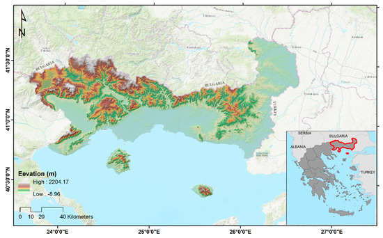
Figure 1.
Location map and digital elevation model (DEM) of the study area.
The average annual temperature recorded over the 1960–1990 period was 16 °C, and the average annual precipitation was 481 mm. REMTH predominantly features a hot-summer Mediterranean climate (Csa) near the coastline, but further into the mainland of the region, and in the Rhodopi mountain range across the Greek–Bulgaria borders, the climate becomes continental, winter is harsh, has no dry season, and has a warm summer (Dfb) [46].
Climatic variability is also reflected in the natural environment of the region. Three altitudinal vegetation zones were recognized. The first vegetation zone (Quercetalia ilicis) in the study area is located above sea level to an altitude of 200–300 m. In this area, the vegetation zone is represented by the sub-zone Quercion ilicis, in which various plant communities appear that are partly degraded and partly territorially dependent (permanent plant communities). The floristic composition of these communities species is involved species such as Erica manipuliflora, Erica arborea, Arbutus unedo, Calicotome villosa, Spartium junceum, Quercus ilex, Fraxinus ornus, Phillyrea latifolia, Quercus pubescens, etc. This subzone is optimum for the growth of Pinus halepensis ssp. halepensis, as well as its Pinus halepensis ssp. brutia. The second vegetation zone (Quercetalia pubescentis) in the study area is located above the previous one and up to an altitude of 1000 m. The vegetation zone has 3 sub-zones in Greece, with 2 in the study area. The first sub-zone is Ostryo-Carpinion, which includes species such as Quercus cocciferra, Carpinus orientalis, Fraxinus ornus, Pistacia terebinthus, Ligustrum vulgare, Rhus coriaria, Cotinus coggygria, Quercus pubescens, Quercus frainetto, Acer monspessulanum, Sorbus torminalis, etc. The second sub-zone that is above the previous sub-zone is Quercion confertae and includes the oak forests of the area, also with the presence of species Castanea sativa, Tilia tomentosa, Acer obtusatum, Ostrya carpinifolia, Carpinus betulus, etc. The third vegetation zone (Fagetalia) in the study area is located above the previous one and up to the altitude of 1800 m. This vegetation zone has two sub-zones, but only one is present in the study area (Fagion moesiacae). The vegetation zone includes the forest of Pinus nigra, Fagus sylvatica, and Abies borisii-regis. The fourth vegetation zone (Vaccinio-Picetalia) is represented by the sub-zone Vaccinio-Piceion, which is located across the forest lines and includes the forest of Picea abies. The last vegetation zone (Astragalo-Acantholimonetalia) is located above the forest lines and includes grasslands that degraded due to overgrazing because these lands serve as summer pastures for herds [47,48,49].
2.2. Methodological Analysis Outline
For the development of the fuel type maps, three main steps were followed. At the first step, fuel type scheme development relied on field reconnaissance and measurements, as well as manual interpretation of VHR base maps (Google Earth) and existing auxiliary vegetation maps. The second step involved Sentinel-2 and Sentinel-1 dataset preprocessing, spectral information enhancement, backscattering information retrieval, and topographic variables extraction. In the third step, three models were developed using different datasets. The final step of the workflow was the classification accuracy assessment along with the variable importance analysis rating. The overall process diagram of the methodology used in the current research is shown in Figure 2.
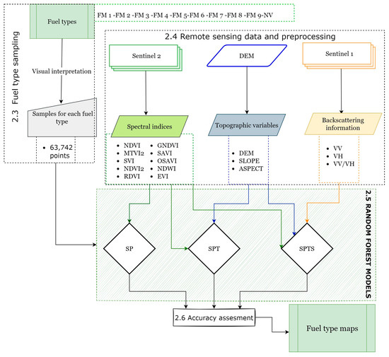
Figure 2.
General process flow diagram: spectral index model (SP); spectral index and topographic variables model (SPT); spectral indices and topographic variables and backscatter information model (SPTS).
2.3. Fuel Type Sampling
The forest fuel type classification scheme includes nine fuel models (FM) (Table 1). The nine-class scheme was specified considering fire behavior modeling requirements, vegetation diversity within REMTH, and the need to adopt a simple and reproducible scheme for future updates. The successional stages, time since disturbance, and stand-specific characteristics (i.e., forest age) were not considered during scheme development to avoid complexity and increase confidence in the mapping workflow. An additional class (NV) was added to account for those areas without vegetation or other land uses (water, burnt areas, urban areas, bare soil, crops, irrigated crops, and floodplains).

Table 1.
Fuel models of the study area.
Fuel parameters were determined following the field sampling procedures described by Mallinis et al. [18]. In brief, the methodology developed by Brown et al. (1982) [50] for inventorying biomass was used in representative, homogeneous fuel plots. The sampling approach included both 30 m transects (for the 1 h, 10 h, 100 h, 1000 h, and total fuel loads) and 100 m2 square plots (for the herbaceous (live and dead) and shrub vegetation loads, foliage load, litter load, and depth).
A total of 63,742 sample points (Figure 3) were collected using visual image interpretation, utilizing recent very high spatial resolution (up to 0.5 m) satellite imagery, available via Web Map Service (WMS) standards, and vegetation and land-use maps from Greek Ministry of Environment and Energy. Vegetation and land-use maps, as a key part of forest management studies at a scale of 1:20,000, provide information on the distribution of forest species within the forest areas of the study area. The number of samples per fuel type and their spatial distribution are presented in Figure 3.
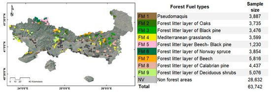
Figure 3.
Fuel type sampling: sample points locations superimposed on Sentinel-2 imagery (left); forest fuel types (right).
2.4. Remote Sensing Data and Preprocessing
Sentinel-2 surface reflectance products (L2A) were acquired on August 2021, and a monthly composite with average values was created within the Google Earth Engine (GEE) environment to fully cover the spatial extent of the region of REMTH. A series of spectral indices (Table 2) were considered as potential predictors based on finding of previous fuel mapping [51] or vegetation mapping studies [52,53].
Table 2.
Mathematic formula and motivation for considering each spectral index in the fuel type classification process.
Sentinel-1 images were also retrieved and processed using the GEE platform [67]. Sentinel-1 C-band images of interferometric wide swath mode, VV (vertical transmit–vertical receive) and VH (vertical transmit–horizontal receive) polarizations, acquired in August 2021. The Sentinel-1 data were initially calibrated into σ0 backscatter coefficient values (Equations (1)) and despeckled using a 5 × 5 Lee filter.
By default, the Shuttle Radar Topography Mission (SRTM) digital elevation model, at a resolution of 1 arc-second (∼30 m) [68], available as a GEE asset, was used for terrain correction [69]. Finally, the Sentinel-1 mosaic with VH and VV polarization bands covering the study area was used for the ratio (VV/VH) calculation (Equation (2)).
Information on the topography was derived from the digital elevation model (DEM) for Europe (EU-DEM) created for the Copernicus programme at a 25 m spatial resolution [70]. Elevation, slope, and aspect were incorporated into the analysis process.
2.5. Classification Models
The random forest (RF) classification algorithm [71], a non-parametric, tree-based classifier, was employed for fuel type classification. To investigate the optimal approach, three different RF models were developed using the following datasets (Table 3):
Table 3.
Variables of random forest models: spectral index model (SP); spectral index and topographic variables model (SPT); spectral indices and topographic variables and backscatter information model (SPTS).
- Spectral indices model (SP) using the 10 spectral indices;
- Spectral indices and topographic variables model (SPT) using 13 variables;
- Spectral indices, topographic, and backscatter information (SPTS) model using 16 variables.
The “randomForest” [72] and “caret” [73] packages were used for developing an end-to-end processing workflow (training, prediction, and mapping) within R environment software [74].
The reference data were split into training and test data samples with a ratio of 70:30 using random stratified sampling to include the different fuel types. In the modeling process, two-thirds of the train data were used while one-third (out-of-bag samples (OOB)) were used for model validation, calculating the out-of-bag (OOB) estimate of error rate [71]. RF was operated with default settings for the number of input variables at each split ((mtry) equal to the square root of the number of input variables at each node), the node size was set to the default value of 5, and the number of trees to grow (ntrees) was set to 1000.
2.6. Accuracy Assessment
For the validation process and the RF performance, the test data were used along with the reference data collected during the field survey. For the accuracy assessment, the confusion matrix for the actual and predicted fuel type identities’ overall accuracy (OA) [75], user’s accuracy (UA) [75], producer’s accuracy (PA) [75], kappa and weighted kappa statistic [76], and the out-of-bag (OOB) estimate of error rate were also reported. User’s accuracy (UA) represents the proportion of classified sample plots that correctly represents that category on the ground. Producer’s accuracy (PA) describes how well features on the ground are correctly classified on a map [29,75]. Overall accuracy (OA) is calculated by dividing the total correctly classified sample by the total number of observations [29,75]. The kappa statistic reflects the difference between observed agreement and agreement expected by random chance [77]. The weighted kappa takes into consideration the different levels of disagreement between categories [78]. The OOB error is the OOB estimate of the error rate [71]. Moreover, McNemar’s test [79] was performed to statistically compare error matrices of the three developed models, focused on the binary distinction between correct and incorrect class allocations (Equation (3)) [80].
A difference in accuracy between the confusion matrices of the classifiers is statistically significant (p ≤ 0.05) if the Z value is more than 1.96 [80].
2.7. Variable Importance
Furthermore, the relative importance of each variable was examined by calculating the mean decrease in accuracy (MDA). The MDA measure implemented in the RF classifier is the most well-known measure to estimate variable importance [81,82]. MDA is a straightforward technique [83,84] derived from the idea that if the variable is not important, then rearranging its values should not reduce prediction accuracy [85]. MDA is calculated by averaging the difference in OOB error before and after one variable is randomly permutated from the analysis.
3. Results
3.1. Forest Fuel Type Classification
The results indicate the SPTS model as the most accurate model, with overall accuracy (OA) of 92.76%, followed by SPT (OA = 91.92%) and SP (OA = 81.39%). Accuracy metrics are presented in Table 4, and the resulting maps generated by the three models are illustrated in Figure 4. McNemar’s test was applied to assess whether statistically significant differences between classifications exist. In particular, based on McNemar’s test, there was a significant difference (Z >1.96) at the 5% significance level between the confusion matrices of the SP, SPT, and SPTS.
Table 4.
Fuel type classification accuracy for the spectral indices model (SP); spectral indices and topography model (SPT); and spectral indices, topography, and backscatter information model (SPTS).
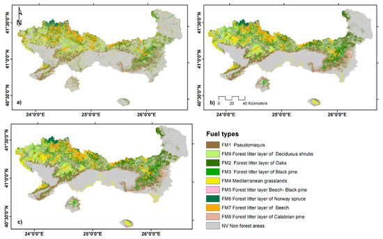
Figure 4.
Fuel type maps resulting from the different classification models: (a) Spectral indices model (SP); (b) spectral indices and topography model (SPT); (c) Spectral indices, topography, and backscattering information (SPTS) model.
3.1.1. Spectral Indices Model
Regarding the fuel-type map produced by the SP model, the results indicate overall accuracy OA (81.39%) (Table 4). In terms of the individual classes’ accuracy (Table 5), certain issues were detected in the class of FM4 Mediterranean grassland, which was erroneously assigned in other classes (PA = 44.23%) and mainly in other uses (NV). This can be partially related to the fact that the NV class also includes agricultural land, which may be spectrally similar to grassland cover. Misclassifications were also noticed for type FM5 forest litter layer beech–black pine (PA = 46.80%), which is confused with the FM6 forest litter layer of Norway spruce and FM7 forest litter layer of beech, and this is obviously due to the mixing rate of type FM5 forest litter layer beech–black pine. Errors also occur between the FM3 forest litter layer of black pine and the FM8 forest litter layer of Calabrian pine. Moreover, the FM7 forest litter layer of beech shows the highest accuracies.
Table 5.
Confusion matrix for the spectral indices (SP) model: values are given in percentage of validation points.
3.1.2. Spectral Indices and Topographic Variables Model
Compared to the SP model, the SPT model showed higher overall accuracy (OA = 91.92%) (Table 4). According to the confusion matrix (Table 6), the greatest confusion is between the fuel types FM5 forest litter layer beech–black pine and FM7 forest litter layer of beech, as well as FM3 forest litter layer of black pine and FM8 forest litter layer of Calabrian pine. Even though the underestimation of FM5 forest litter layer beech–black pine still remained (PA 59.33%, UA 87.30%), the accuracy results have improved compared to those of the SP model, with a significant increase in accuracy in the classification of FM4 Mediterranean grasslands type (PA = 82.99% and UA = 96.59%) and FM1 pseudomaquis (PA = 86.69% and UA = 81.89%), demonstrating the importance of topographic variables in the fuel type classification model.
Table 6.
Confusion matrix for the spectral index and topographic variables (SPT) model: values are given in percentage of validation points.
3.1.3. Spectral Indices, Topography, and Backscattering Information Model (SPTS)
The SPTS model accuracies show a clear improvement over the SP model and a slight increase over the SPT model (OA = 92.76%) (Table 4). According to the confusion matrix (Table 7) and comparing to SPT models (Table 6), Sentinel-1 predictors improved the separability of the FM5 forest litter layer beech–black pine from the F7 forest litter layer of beech and of FM4 Mediterranean grasslands from NV non-forest areas. Moreover, the inclusion of backscattering information indicates an improvement in discrimination of the FM8 forest litter layer of Calabrian pine from FM1 pseudomaquis and NV non-forest-areas, of FM1 pseudomaquis from FM8 forest litter layer of Calabrian pine, and of FM3 forest litter layer of black pine from FM1 Pseudomaquis. However, confusion still remained in the FM5 forest litter layer beech–black pine, which was misclassified to other fuel types (PA = 59.33%) and mainly as the FM7 forest litter layer of beech. Overall, with the exception of FM5 Forest litter layer beech–black pine, the remaining categories were classified with PA and UA accuracies exceeding 80%.
Table 7.
Confusion matrix for spectral indices, topographic variables, and backscattering information (SPTS) model. Values are given in percentage of validation points.
In general, FM1 pseudomaquis, FM7 forest litter layer of beech, NV non-forest areas class presented overestimations (Figure 5), FM3 forest litter layer of black pine, FM4 Mediterranean grasslands, and FM5 forest litter layer beech–black pine were underestimated, albeit presenting high PAs and UAs, respectively.
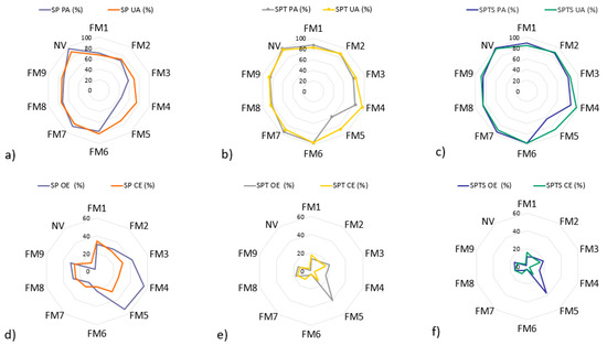
Figure 5.
Comparing producers’ (PA) and users’ (UA) accuracies (first row), commission (CE) and omission errors (OE) (second row) of the three models: spectral index (SP) model; spectral index and topographic variables (SPT); spectral indices, topographic variables, and backscatter information (SPTS) model. (a) producers’ (PA) and users’ (UA) accuracies of spectral index (SP) model, (b) producers’ (PA) and users’ (UA) accuracies of spectral index and topographic variables (SPT) model, (b) producers’ (PA) and users’ (UA) accuracies of spectral index and topographic variables (SPT) model (c) producers’ (PA) and users’ (UA) accuracies of spectral indices, topographic variables, and backscatter information (SPTS) model, (d) commission (CE) and omission errors (OE) of spectral index (SP) model, (e) commission (CE) and omission errors (OE) of spectral index and topographic variables (SPT) model, (f) commission (CE) and omission errors (OE) of spectral indices, topographic variables, and backscatter information (SPTS) model.
3.2. Visual Inspection
For visual inspection of the maps, a representative area with different topography and tree species composition was selected. Figure 6 illustrates that the largest differences were obtained between SP and SPT or SPTS model. In this case of SP, the RF predictions also seemed to be noisier, underestimating the FM4 Mediterranean grasslands and overestimating FM1 pseudomaquis. The spatial patterns of fuel types are quite similar when using SPT or SPTS model; however, the separability of FM5 forest litter layer beech–black pine from the F7 forest litter layer of beech is improved on the SPTS model.
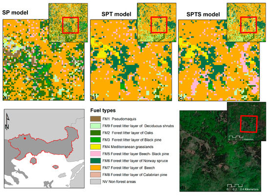
Figure 6.
Closeup of classifications for the three models: (a) spectral indices (SP) model; (b) spectral indices and topography (SPT) model; (c) spectral indices, topography, and backscattering information (SPTS) model; (d) Google Earth imagery.
3.3. Variable Importance
The SP and SPT models were disregarded for subsequent analysis as they presented lower overall accuracies. In this sense, the SPTS model included 16 variables and was selected for further analysis of variable importance. The variable importance of SP and SPT models is given in Appendix A (Figure A1).
The importance of each variable was assessed using a mean decrease in accuracy (MDA) measure provided by the RF model. Figure 7 shows the variable importance ranking of the SPTS model based on MDA statistics. Relating to the MDA statistics (Figure 7), the most significant variables are the DEM and aspect, SVI and NDWI, and backscattering information, which were included in the seven most significant variables.
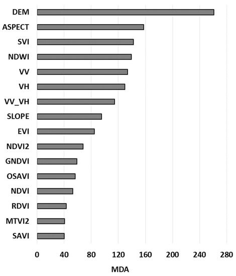
Figure 7.
Variable importance ranking of spectral indices, topographic variables, and backscattering information model (SPTS) based on mean decrease accuracy (MDA).
Boxes chart for backscatter (Figure 8) and spectral (Figure 9) profile of fuel type samples were developed to highlight the similarity of the fuel type classes.
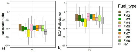
Figure 8.
Boxes chart for backscatter profile of fuel type samples: (a) VV polarization, (b) VH polarization.
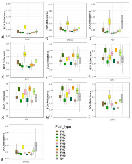
Figure 9.
Boxes chart for spectral profile of fuel type samples: (a) blue band, (b) green band (c) red band, (d) red edge 1 band, (e) red edge 2 band, (f) near-infrared narrow 1 band, (g) near-infrared band, (h) near-infrared narrow 2 band, (i) short wavelength 1 band, (j) short wavelength 1 band.
4. Discussion
4.1. Fuel Type Classification Model’s Comparison
Wildfire is one of the main processes affecting the dynamics of Mediterranean forests [35]. An accurate and regularly updated description of the spatial distribution of wildland fuels is crucial for forest fuel management, fire management, firefighting, and mitigation of environmental and economic threats. Fuel mapping is essential for predicting fire behavior and managing vegetation, while wildfire behavior is partly determined by stand structure, composition, and vegetation characteristics. Currently, categorical fuel types corresponding to major forested vegetated/forested types are being used globally for fire research and management applications [86,87,88,89].
The strength of data fusion for forest type or fuel type classification has been successfully evaluated by many studies, but very few specifically addressed wildland fuel type mapping with the synergetic use of Sentinel-2, Sentinel-1 data, and topographic information. Most of these studies relied on the combined use of LiDAR with optical data [20,90]. The present work mapped vegetation/forest types implying categorical fuel types in a heterogeneous landscape of Northern Greece, combining three different datasets: Sentinel-2 spectral indices, topography, and Sentinel-1 backscattering information.
Optical data alone achieved less satisfactory results. The higher omission error noted in the case of FM4 Mediterranean grasslands, FM3 forest litter layer of black pine, and FM5 forest litter layer beech–black-pine is mainly related to the spectral similarity of these types with the NV non-forest areas, FM8 forest litter layer of Calabrian pine and FM6 forest litter layer of Norway spruce, and FM7 forest litter layer of beech, respectively.
Topographic variables included in the SPT model enhanced classification accuracy for all fuel types. Previous research related to vegetation patterns [34,91,92] and cover estimation [93] have also identified the influence of topography. In our case, the most noticeable improvement was observed for the FM3 forest litter layer of black pine, FM4 Mediterranean grasslands, and FM6 forest litter layer of Norway spruce. In Mediterranean areas, black pine generally colonizes areas at higher altitudes [94]; thus, the elevation predictor improved the FM3 forest litter layer of black pine separability from other fuel types on lower altitudes such as FM1 pseudomaquis, FM9 forest litter layer of deciduous shrubs, and NV non-forest areas. Topographic variables also supported the separability of FM4 Mediterranean grasslands from NV non-forest areas, as agricultural land occupies land on lower elevations. Similarly, the FM6 forest litter layer of Norway spruce gains classification accuracy due to topography-related variables since Norway spruce occupies higher altitude areas of the Rhodope Mountain range. However, misclassifications were noted again, especially in FM5 forest litter layer beech–black pine, due to spectral similarity with other classes.
The microwave energy of the C-band is mainly affected by the structural properties of a forest, such as the size, orientation, and spatial pattern of trees as a whole, and it scattered back to the sensor from the upper tree crown, branches, and leaves, and less from beneath [95]; thus, C-band backscatter signals are sensitive to forest biomass forest structure and vegetation water content [96,97]. Consequently, SAR predictors support the discrimination of forest/non-forest [98] areas as well different forest types of vegetation types with different water content and structure [29]. The synergetic use of optical and topographic variables with backscattering information slightly improved classification accuracy mostly of the FM5 forest litter layer beech–black pine, FM8 forest litter layer of Calabrian pine, FM1 pseudomaquis, FM4 Mediterranean grasslands, and FM3 forest litter layer of black pine. In the present study, FM5 forest litter layer beech–black pine was the most difficult class to map because, depending on the forest mix rate at the pixel level, the class shares spectral similarities with the FM7 forest litter layer of beech and FM3 forest litter layer of black pine [99]. However, Sentinel-1 variables contributed, even slightly, to separate these fuel types due to different canopy roughness and stand height between mixed and single species stands.
4.2. Variable Importance
With respect to variable importance ranking, the results demonstrate that all three datasets provide valuable information on fuel type properties; the MDA statistic indicates that not all variables contributed equally to the tree species classification.
Topographic metrics, mainly the aspect of the slope and altitude, have a considerable role in vegetation composition [100] and can distinguish different tree species [101]. The highest rank observed for elevation has been related in numerous studies to the altitudinal zonation of vegetation groups [32]. The high contribution of DEM was also confirmed by previous research on land cover classification [33,102] and tree species separability [101]. Aspect is presented as the second most important variable, as it is related to vegetation differences mainly due to differential exposure to the sun. Moreover, herb biomass significantly differed between aspects [100].
Concerning the slope, the south-facing slopes are drier than the north-facing slopes [103]. The wet and cool north-facing slopes are indirectly exposed to the sun and present low-intensity north-east rains during the winter season, thus holding more water and providing suitable conditions for the moisture-loving tree species [103]. Slope is also related to solar radiation across the surface, runoff, and gravity flow, all of which contribute to the presence of individual tree species as well as their number [104]; for instance, steep slopes are generally associated with broadleaves due to their developed root system [32], agricultural land and urban areas are usually located in relatively flat areas, and some tree species are likely to appear in sunny or shady-slope areas [105].
In regard to the highest-ranking spectral indices SVI and NDWI have a special interest in the classification of fuel types proving the importance of NIRn2, RE2, and SWIR spectral bands. Normalized difference water index (NDWI) as a common wetness index is sensitive to changes in the vegetation moisture content [106] and is often used in fire-related [107,108] and forest parameters studies [109,110]. Previous research proves that NDWI presents good spectral proxies for variations in vegetation density [111], and there is a correlation between NDWI and live fuel moisture content [25], facts that are associated with forest fuel type. Previous studies also use SVI for fuel type mapping [51]. The importance score noted for SVI supports the major role of the NIR (B8) and the red edge 2 (B6) bands of Sentinel imagery for forest fuel classification. SVI is a slight alteration to the traditional NDVI and considers a narrower waveband at the edge of the chlorophyll absorption feature (e.g., 740 nm), where the spectrum is characterized by lower absorption by chlorophyll, reducing the saturation effect. However, the reflectance still remains sensitive to chlorophyll absorption at its moderate-to-high values [112,113], and the sensitivity of the VI is enhanced to moderate–high vegetation densities [114], which is associated with forest fuel load and type.
Regarding backscattering information, Sentinel-1 variables improve the separability in classes that vary in terms of height (e.g., FM8 forest litter layer of Calabrian pine and FM3 forest litter layer of black pine from FM1 pseudomaquis and NV non-forest areas), or density (e.g., FM5 forest litter layer beech–black pine from FM7 forest litter layer of beech, and of FM4 Mediterranean grasslands from NV non-forest areas). Polarisation VV and VH present similar importance in terms of MDA; however, VV was rated slightly more important than VH in fuel type classification. VV backscatter is usually linked both to water content and surface roughness [115] and is dominated by direct contributions from the ground and the canopy [116]. VV polarization also performs better than VH polarization in land cover classification [117]. In contrast, in other studies, VH predictors have been proven to be more sensitive to tree/forest structure than VV predictors [95,118]; however, leaf-on SAR images used in the present study may influence the importance ranking of backscattering polarization because the leaves-on season both deciduous and evergreen contributes to crown volumetric scattering [115]. Ratio VV/VH was less important than the two polarisations since VV/VH reduces the dependence of the radar signal on soil moisture [119].
4.3. Limitations and Further Research Perspectives
The specific aim of this study was to investigate the synergistic use of Sentinel-2, Sentinel-1, and topography in classifying vegetation/forest types, as well as to explore the relative importance of spectral indices, backscattering, and topography information for an easy-to-update categorical fuel type mapping.
Our study considered static, structural, and single-month spectral characteristics of vegetation. Unfortunately, such variables restrict estimates of seasonal variations in phenologies. Vegetation phenology could provide important information on the successful discrimination of the fuel types [120] since phenological characteristics such as moisture content, leaf biomass, and chemical composition affect plant flammability. Future research should aim to investigate the potential of multi-temporal Sentinel-1 and Sentinel-2 datasets to develop a phenological fuel map considering the seasonality and inter-annual variability of forest fuel.
This study aimed to achieve a simple and robust model by using spectral indices, which have been used successfully for fuel mapping [51] and vegetation mapping [52,53] in previous studies. However, spectral data analysis is an important tool for classification problems [121], yet the choice of a suitable spectral index needs more consideration since it is contingent upon the specific application and environmental conditions [122]. Thorough research on the spectral profile of forest fuel types, as well as on spectral band importance in forest fuel mapping, could provide additional information to fuel type mapping, improve understanding of spectral indexes, and develop new effective spectral indexes.
A further point to be considered in future studies is the transferability of the model. The spatial variability of fuel types, along with uncertainties related to satellite imagery preprocessing, constrain model transferability between different areas. Overall, the developed regional model is currently specific to REMTH, but the general methodology is transferable to any other area with similar environmental characteristics. For improving the spatial transferability of fuel type classification models, future research might also evaluate the effectiveness of optical and SAR texture variables or features such as folded aspect [123] or vegetation management indicators that are independent of phenological stages. Finally, the development and delineation of a more detailed fuel type classification scheme, also considering successional stages and time since disturbance could facilitate fire behavior modeling, albeit it will be more challenging at extended scales requiring additional complementary information from LiDAR sensors [124].
The originality of this study methodology resides in the utility of Sentinel-1 data for the spatial distribution maps of wildland fuel in a Mediterranean landscape. The combination of information arising from backscattering data, optical data, and topographic metrics appears to be promising for accurate forest fuel mapping. The results obtained can also be used to guide the selection of suitable variables to develop an accurate fuel type classification model in a regional setting approach. Moreover, the developed models can be easily updated with newly available data, supporting decision-makers and disaster management with the necessary spatially distributed information on fuel types over the region.
5. Conclusions
Up-to-date mapping of fuel types is vital for wildland fire prevention. This study aimed to evaluate the synergetic use of three different datasets to develop accurate vegetation fuel maps and investigated the relative importance of spectral indices, backscattering information, and topography in fuel type mapping in a Mediterranean environment in Southern Greece.
In summary, the conclusions of this study are:
- The SPTS model yielded the highest overall accuracy (OA) of 92.76%, followed by SPT (OA = 91.92%) and SP (OA = 81.39%);
- The Sentinel-2 spectral indices produce accurate maps of forest fuel types;
- Topographic variables enhance model performance;
- Sentinel-1 data have a positive influence on the accuracy of forest fuel type classification;
- Variable importance measures highlighted the importance of the digital elevation model.
Overall, the results of this study provide evidence that encourages the synergistic use of Sentinel-2, Sentinel-1, and topography variables in fuel type mapping. Future work will involve the application of the generated fuel map as a key aspect of fire risk assessment across the region of East Macedonia and Thrace, providing automatic production of reliable results on fuel mapping and fire behavior at an operational level.
Author Contributions
Conceptualization, G.M.; methodology, G.M. and I.C.; field data acquisition, C.D.; data analysis I.C.; writing—original draft preparation I.C. and G.M.; writing—review and editing, C.D., V.G. and I.M.; supervision, G.M.; project administration, I.M.D.; funding acquisition, I.M.D. All authors have read and agreed to the published version of the manuscript.
Funding
We acknowledge support of this work by the project “Risk and Resilience Assessment Center–Prefecture of East Macedonia and Thrace-Greece” (MIS 5047293) which is implemented under the Action “Reinforcement of the Research and Innovation Infrastructure”, funded by the Operational Programme “Competitiveness, Entrepreneurship and Innovation” (NSRF 2014-2020) and co-financed by Greece and the European Union (European Regional Development Fund).
Institutional Review Board Statement
Not applicable.
Informed Consent Statement
Not applicable.
Data Availability Statement
Data sharing not applicable.
Acknowledgments
We acknowledge the support of this work by the project “Risk and Resilience Assessment Center—Prefecture of East Macedonia and Thrace -Greece.” (MIS 5047293), which is implemented under the Action “Reinforcement of the Research and Innovation Infrastructure”.
Conflicts of Interest
The authors declare no conflict of interest.
Appendix A

Figure A1.
Variable importance ranking of (a) spectral indices model (SP) and (b) spectral indices and topographic variables model (SPT), based on mean decrease accuracy (MDA).
References
- Pausas, J.G.; Keeley, J.E.; Schwilk, D.W. Flammability as an Ecological and Evolutionary Driver. J. Ecol. 2017, 105, 289–297. [Google Scholar] [CrossRef]
- Turco, M.; Bedia, J.; Di Liberto, F.; Fiorucci, P.; von Hardenberg, J.; Koutsias, N.; Llasat, M.-C.; Xystrakis, F.; Provenzale, A. Decreasing Fires in Mediterranean Europe. PLoS ONE 2016, 11, e0150663. [Google Scholar] [CrossRef]
- Jones, G.M.; Tingley, M.W. Pyrodiversity and Biodiversity: A History, Synthesis, and Outlook. Divers. Distrib. 2022, 28, 386–403. [Google Scholar] [CrossRef]
- Christopoulou, A.; Mallinis, G.; Vassilakis, E.; Farangitakis, G.-P.; Fyllas, N.M.; Kokkoris, G.D.; Arianoutsou, M. Assessing the Impact of Different Landscape Features on Post-Fire Forest Recovery with Multitemporal Remote Sensing Data: The Case of Mount Taygetos (Southern Greece). Int. J. Wildl. Fire 2019, 28, 521. [Google Scholar] [CrossRef]
- Pausas, J.G.; Keeley, J.E. A Burning Story: The Role of Fire in the History of Life. Bioscience 2009, 59, 593–601. [Google Scholar] [CrossRef]
- Taboada, A.; García-Llamas, P.; Fernández-Guisuraga, J.M.; Calvo, L. Wildfires Impact on Ecosystem Service Delivery in Fire-Prone Maritime Pine-Dominated Forests. Ecosyst. Serv. 2021, 50, 101334. [Google Scholar] [CrossRef]
- Moore, P.F. Global Wildland Fire Management Research Needs. Curr. For. Rep. 2019, 5, 210–225. [Google Scholar] [CrossRef]
- San-Miguel-Ayanz, J.; Durrant, T.; Boca, R.; Maianti, P.; Libertá, G.; Artés-Vivancos, T.; Oom, D.; Branco, A.; de Rigo, D.; Ferrari, D.; et al. Forest Fires in Europe, Middle East and North Africa 2021; Publications Office of the European Union: Luxembourg, 2022. [Google Scholar]
- Rodrigues, M.; Cunill Camprubí, À.; Balaguer-Romano, R.; Coco Megía, C.J.; Castañares, F.; Ruffault, J.; Fernandes, P.M.; Resco de Dios, V. Drivers and Implications of the Extreme 2022 Wildfire Season in Southwest Europe. Sci. Total Environ. 2023, 859, 160320. [Google Scholar] [CrossRef]
- Hanan, E.J.; Ren, J.; Tague, C.L.; Kolden, C.A.; Abatzoglou, J.T.; Bart, R.R.; Kennedy, M.C.; Liu, M.; Adam, J.C. How Climate Change and Fire Exclusion Drive Wildfire Regimes at Actionable Scales. Environ. Res. Lett. 2021, 16, 24051. [Google Scholar] [CrossRef]
- Oom, D.; de Rigo, D.; Pfeiffer, H.; Branco, A.; Ferrari, D.; Grecchi, R.; Artés-Vivancos, T.; Houston Durrant, T.; Boca, R.; Maianti, P.; et al. Pan-European Wildfire Risk Assessment, EUR 31160 EN; Publications Office of the European Union: Luxembourg, 2022. [Google Scholar]
- National Wildfire Coordinating Group Incident Response Pocket Guide; National Wildfire Coordinating Group, Operations and Training Committee, NWCG PMS: Missoula, MT, USA, 2018; p. 138.
- Mallinis, G.; Mitsopoulos, I.D.; Dimitrakopoulos, A.P.; Gitas, I.Z.; Karteris, M. Local-Scale Fuel-Type Mapping and Fire Behavior Prediction by Employing High-Resolution Satellite Imagery. IEEE J. Sel. Top. Appl. Earth Obs. Remote Sens. 2008, 1, 230–239. [Google Scholar] [CrossRef]
- Keane, R.E.; Burgan, R.; Van Wagtendonk, J. Mapping Wildland Fuels for Fire Management across Multiple Scales: Integrating Remote Sensing, GIS, and Biophysical Modeling. Int. J. Wildl. Fire 2001, 10, 301. [Google Scholar] [CrossRef]
- Arroyo, L.A.; Pascual, C.; Manzanera, J.A. Fire Models and Methods to Map Fuel Types: The Role of Remote Sensing. For. Ecol. Manag. 2008, 256, 1239–1252. [Google Scholar] [CrossRef]
- Chuvieco, E.; Aguado, I.; Salas, J.; García, M.; Yebra, M.; Oliva, P. Satellite Remote Sensing Contributions to Wildland Fire Science and Management. Curr. For. Rep. 2020, 6, 81–96. [Google Scholar] [CrossRef]
- Pettinari, M.L.; Chuvieco, E. Fire Danger Observed from Space. Surv. Geophys. 2020, 41, 1437–1459. [Google Scholar] [CrossRef]
- Mallinis, G.; Galidaki, G.; Gitas, I. A Comparative Analysis of EO-1 Hyperion, Quickbird and Landsat TM Imagery for Fuel Type Mapping of a Typical Mediterranean Landscape. Remote Sens. 2014, 6, 1684–1704. [Google Scholar] [CrossRef]
- Gale, M.G.; Cary, G.J.; Van Dijk, A.I.J.M.; Yebra, M. Forest Fire Fuel through the Lens of Remote Sensing: Review of Approaches, Challenges and Future Directions in the Remote Sensing of Biotic Determinants of Fire Behaviour. Remote Sens. Environ. 2021, 255, 112282. [Google Scholar] [CrossRef]
- Domingo, D.; de la Riva, J.; Lamelas, M.; García-Martín, A.; Ibarra, P.; Echeverría, M.; Hoffrén, R. Fuel Type Classification Using Airborne Laser Scanning and Sentinel 2 Data in Mediterranean Forest Affected by Wildfires. Remote Sens. 2020, 12, 3660. [Google Scholar] [CrossRef]
- Huesca, M.; Riaño, D.; Ustin, S.L. Spectral Mapping Methods Applied to LiDAR Data: Application to Fuel Type Mapping. Int. J. Appl. Earth Obs. Geoinf. 2019, 74, 159–168. [Google Scholar] [CrossRef]
- García, M.; Popescu, S.; Riaño, D.; Zhao, K.; Neuenschwander, A.; Agca, M.; Chuvieco, E. Characterization of Canopy Fuels Using ICESat/GLAS Data. Remote Sens. Environ. 2012, 123, 81–89. [Google Scholar] [CrossRef]
- de Souza Mendes, F.; Baron, D.; Gerold, G.; Liesenberg, V.; Erasmi, S. Optical and SAR Remote Sensing Synergism for Mapping Vegetation Types in the Endangered Cerrado/Amazon Ecotone of Nova Mutum-Mato Grosso. Remote Sens. 2019, 11, 1161. [Google Scholar] [CrossRef]
- Wang, L.; Quan, X.; He, B.; Yebra, M.; Xing, M.; Liu, X. Assessment of the Dual Polarimetric Sentinel-1A Data for Forest Fuel Moisture Content Estimation. Remote Sens. 2019, 11, 1568. [Google Scholar] [CrossRef]
- Fan, L.; Wigneron, J.P.; Xiao, Q.; Al-Yaari, A.; Wen, J.; Martin-StPaul, N.; Dupuy, J.L.; Pimont, F.; Al Bitar, A.; Fernandez-Moran, R.; et al. Evaluation of Microwave Remote Sensing for Monitoring Live Fuel Moisture Content in the Mediterranean Region. Remote Sens. Environ. 2018, 205, 210–223. [Google Scholar] [CrossRef]
- Saatchi, S.; Halligan, K.; Despain, D.G.; Crabtree, R.L. Estimation of Forest Fuel Load from Radar Remote Sensing. IEEE Trans. Geosci. Remote Sens. 2007, 45, 1726–1740. [Google Scholar] [CrossRef]
- D’este, M.; Elia, M.; Giannico, V.; Spano, G.; Lafortezza, R.; Sanesi, G. Machine Learning Techniques for Fine Dead Fuel Load Estimation Using Multi-source Remote Sensing Data. Remote Sens. 2021, 13, 1658. [Google Scholar] [CrossRef]
- Chhabra, A.; Rüdiger, C.; Yebra, M.; Jagdhuber, T.; Hilton, J. RADAR-Vegetation Structural Perpendicular Index (R-VSPI) for the Quantification of Wildfire Impact and Post-Fire Vegetation Recovery. Remote Sens. 2022, 14, 3132. [Google Scholar] [CrossRef]
- Udali, A.; Lingua, E.; Persson, H.J. Assessing Forest Type and Tree Species Classification Using Sentinel-1 C-Band SAR Data in Southern Sweden. Remote Sens. 2021, 13, 3237. [Google Scholar] [CrossRef]
- Tello, M.; Cazcarra-Bes, V.; Pardini, M.; Papathanassiou, K. Forest Structure Characterization from SAR Tomography at L-Band. IEEE J. Sel. Top. Appl. Earth Obs. Remote Sens. 2018, 11, 3402–3414. [Google Scholar] [CrossRef]
- de Jesus, J.B.; Kuplich, T.M. Applications of Sar Data to Estimate Forest Biophysical Variables in Brazil. Cerne 2020, 26, 88–97. [Google Scholar] [CrossRef]
- José Vidal-Macua, J.; Ninyerola, M.; Zabala, A.; Domingo-Marimon, C.; Pons, X. Factors Affecting Forest Dynamics in the Iberian Peninsula from 1987 to 2012. The Role of Topography and Drought. For. Ecol. Manag. 2017, 406, 290–306. [Google Scholar] [CrossRef]
- Verde, N.; Kokkoris, I.P.; Georgiadis, C.; Kaimaris, D.; Dimopoulos, P.; Mitsopoulos, I.; Mallinis, G. National Scale Land Cover Classification for Ecosystem Services Mapping and Assessment, Using Multitemporal Copernicus EO Data and Google Earth Engine. Remote Sens. 2020, 12, 3303. [Google Scholar] [CrossRef]
- Pfeffer, K.; Pebesma, E.J.; Burrough, P.A. Mapping Alpine Vegetation Using Vegetation Observations and Topographic Attributes. Landsc. Ecol. 2003, 18, 759–776. [Google Scholar] [CrossRef]
- Chirici, G.; Scotti, R.; Montaghi, A.; Barbati, A.; Cartisano, R.; Lopez, G.; Marchetti, M.; Mcroberts, R.E.; Olsson, H.; Corona, P. Stochastic Gradient Boosting Classification Trees for Forest Fuel Types Mapping through Airborne Laser Scanning and IRS LISS-III Imagery. Int. J. Appl. Earth Obs. Geoinf. 2013, 25, 87–97. [Google Scholar] [CrossRef]
- García, M.; Riaño, D.; Chuvieco, E.; Salas, J.; Danson, F.M. Multispectral and LiDAR Data Fusion for Fuel Type Mapping Using Support Vector Machine and Decision Rules. Remote Sens. Environ. 2011, 115, 1369–1379. [Google Scholar] [CrossRef]
- Ruiz, L.Á.; Recio, J.A.; Crespo-Peremarch, P.; Sapena, M. An Object-Based Approach for Mapping Forest Structural Types Based on Low-Density LiDAR and Multispectral Imagery. Geocarto Int. 2018, 33, 443–457. [Google Scholar] [CrossRef]
- Dobrinić, D.; Gašparović, M.; Medak, D. Sentinel-1 and 2 Time-Series for Vegetation Mapping Using Random Forest Classification: A Case Study of Northern Croatia. Remote Sens. 2021, 13, 2321. [Google Scholar] [CrossRef]
- Li, Y.; Quan, X.; Liao, Z.; He, B. Forest Fuel Loads Estimation from Landsat Etm+ and Alos Palsar Data. Remote Sens. 2021, 13, 1189. [Google Scholar] [CrossRef]
- Aragoneses, E.; Chuvieco, E. Generation and Mapping of Fuel Types for Fire Risk Assessment. Fire 2021, 4, 59. [Google Scholar] [CrossRef]
- Rego, F.; Rodrigues, J.; Caldaza, V.; Xanthopoulos, G. Forest Fires: Sparking Firesmart Policies in the EU. In Research & Innovation Projects for Policy; Publications Office of the European Union: Luxembourg, 2018. [Google Scholar]
- Marino, E.; Ranz, P.; Tomé, J.L.; Noriega, M.Á.; Esteban, J.; Madrigal, J. Generation of High-Resolution Fuel Model Maps from Discrete Airborne Laser Scanner and Landsat-8 OLI: A Low-Cost and Highly Updated Methodology for Large Areas. Remote Sens. Environ. 2016, 187, 267–280. [Google Scholar] [CrossRef]
- Pyne, J.S. Introduction to Wildland Fire: Fire Management in the United States; John Wiley & Sons: New York, NY, USA, 1984. [Google Scholar]
- McKenzie, D.; Raymond, C.L.; Kellogg, L.-K.B.; Norheim, R.A.; Andreu, A.G.; Bayard, A.C.; Kopper, K.E.; Elman, E. Mapping Fuels at Multiple Scales: Landscape Application of the Fuel Characteristic Classification System. Can. J. For. Res. 2007, 37, 2421–2437. [Google Scholar] [CrossRef]
- Keane, R.E.; Herynk, J.M.; Toney, C.; Urbanski, S.P.; Lutes, D.C.; Ottmar, R.D. Evaluating the Performance and Mapping of Three Fuel Classification Systems Using Forest Inventory and Analysis Surface Fuel Measurements. For. Ecol. Manag. 2013, 305, 248–263. [Google Scholar] [CrossRef]
- Beck, H.E.; Zimmermann, N.E.; McVicar, T.R.; Vergopolan, N.; Berg, A.; Wood, E.F. Present and Future Köppen-Geiger Climate Classification Maps at 1-Km Resolution. Sci. Data 2018, 5, 180214. [Google Scholar] [CrossRef] [PubMed]
- Mavrommatis, G. The Bioclimate of Greece, Relationships between Climate and Natural Vegetation, Bioclimatic Maps. In Dasiki Erevna, Vol. 1, Appendix; Scientific Research Publishing: Athens, Greece, 1980. (In Greek) [Google Scholar]
- Athanasiadis, N. Forest Phytosociology; Giahoudis-Giapoulis: Thessaloniki, Greece, 1986. (In Greek) [Google Scholar]
- Dafis, S. Classification of the Forest Vegetation of Greece; Faculty of Agriculture Forestry, Aristotle University of Thessaloniki: Thessaloniki, Greece, 1973. (In Greek) [Google Scholar]
- Brown, J.K.; Oberheu, R.D.; Johnston, C.M. Handbook for Inventorying Surface Fuels and Biomass in the Interior West; Gen. Tech. Rep. INT-129; U.S. Department of Agriculture, Forest Service, Intermountain Forest and Range Experimental Station: Ogden, UT, USA, 1982; p. 48. [Google Scholar]
- Stefanidou, A.; Gitas, I.Z.; Katagis, T. A National Fuel Type Mapping Method Improvement Using Sentinel-2 Satellite Data. Geocarto Int. 2020, 37, 1022–1042. [Google Scholar] [CrossRef]
- Du, Y.; Zhang, Y.; Ling, F.; Wang, Q.; Li, W.; Li, X. Water Bodies’ Mapping from Sentinel-2 Imagery with Modified Normalized Difference Water Index at 10-m Spatial Resolution Produced by Sharpening the Swir Band. Remote Sens. 2016, 8, 354. [Google Scholar] [CrossRef]
- Bannari, A.; Morin, D.; Bonn, F.; Huete, A.R. A Review of Vegetation Indices. Remote Sens. Rev. 1995, 13, 95–120. [Google Scholar] [CrossRef]
- Rouse, J.W.; Haas, R.H.; Schell, J.A.; Deering, D.W. Monitoring the Vernal Advancement and Retrogradation (Green Wave Effect) of Natural Vegetation; NASA/GSFCT Type II Report; Goddard Space Flight Center: Greenbelt, MD, USA, 1973; p. 86. [Google Scholar]
- Huete, A.; Didan, K.; Miura, T.; Rodriguez, E.P.; Gao, X.; Ferreira, L.G. Overview of the Radiometric and Biophysical Performance of the MODIS Vegetation Indices. Remote Sens. Environ. 2002, 83, 195–213. [Google Scholar] [CrossRef]
- Gao, B.C. NDWI—A Normalized Difference Water Index for Remote Sensing of Vegetation Liquid Water from Space. Remote Sens. Environ. 1996, 58, 257–266. [Google Scholar] [CrossRef]
- Huete, A. A Soil-Adjusted Vegetation Index (SAVI). Remote Sens. Environ. 1988, 25, 295–309. [Google Scholar] [CrossRef]
- Rondeaux, G.; Steven, M.; Baret, F. Optimization of Soil-Adjusted Vegetation Indices. Remote Sens. Environ. 1996, 55, 95–107. [Google Scholar] [CrossRef]
- Gitelson, A.A.; Kaufman, Y.J.; Merzlyak, M.N. Use of a Green Channel in Remote Sensing of Global Vegetation from EOS- MODIS. Remote Sens. Environ. 1996, 58, 289–298. [Google Scholar] [CrossRef]
- Barati, S.; Rayegani, B.; Saati, M.; Sharifi, A.; Nasri, M. Comparison the Accuracies of Different Spectral Indices for Estimation of Vegetation Cover Fraction in Sparse Vegetated Areas. Egypt. J. Remote Sens. Sp. Sci. 2011, 14, 49–56. [Google Scholar] [CrossRef]
- Roujean, J.-L.; Breon, F.-M. Estimating PAR Absorbed by Vegetation from Bidirectional Reflectance Measurements. Remote Sens. Environ. 1995, 51, 375–384. [Google Scholar] [CrossRef]
- Mutanga, O.; Adam, E.; Cho, M.A. High Density Biomass Estimation for Wetland Vegetation Using Worldview-2 Imagery and Random Forest Regression Algorithm. Int. J. Appl. Earth Obs. Geoinf. 2012, 18, 399–406. [Google Scholar] [CrossRef]
- Ng, W.-T.; Rima, P.; Einzmann, K.; Immitzer, M.; Atzberger, C.; Eckert, S. Assessing the Potential of Sentinel-2 and Pléiades Data for the Detection of Prosopis and Vachellia Spp. in Kenya. Remote Sens. 2017, 9, 74. [Google Scholar] [CrossRef]
- Haboudane, D. Hyperspectral Vegetation Indices and Novel Algorithms for Predicting Green LAI of Crop Canopies: Modeling and Validation in the Context of Precision Agriculture. Remote Sens. Environ. 2004, 90, 337–352. [Google Scholar] [CrossRef]
- Feng, W.; Wu, Y.; He, L.; Ren, X.; Wang, Y.; Hou, G.; Wang, Y.; Liu, W.; Guo, T. An Optimized Non-Linear Vegetation Index for Estimating Leaf Area Index in Winter Wheat. Precis. Agric. 2019, 20, 1157–1176. [Google Scholar] [CrossRef]
- Shen, X.; Cao, L.; Yang, B.; Xu, Z.; Wang, G. Estimation of Forest Structural Attributes Using Spectral Indices and Point Clouds from UAS-Based Multispectral and RGB Imageries. Remote Sens. 2019, 11, 800. [Google Scholar] [CrossRef]
- Gorelick, N.; Hancher, M.; Dixon, M.; Ilyushchenko, S.; Thau, D.; Moore, R. Google Earth Engine: Planetary-Scale Geospatial Analysis for Everyone. Remote Sens. Environ. 2017, 202, 18–27. [Google Scholar] [CrossRef]
- Farr, T.G.; Rosen, P.A.; Caro, E.; Crippen, R.; Duren, R.; Hensley, S.; Kobrick, M.; Paller, M.; Rodriguez, E.; Roth, L.; et al. The Shuttle Radar Topography Mission. Rev. Geophys. 2007, 45, RG2004. [Google Scholar] [CrossRef]
- Mullissa, A.; Vollrath, A.; Odongo-Braun, C.; Slagter, B.; Balling, J.; Gou, Y.; Gorelick, N.; Reiche, J. Sentinel-1 Sar Backscatter Analysis Ready Data Preparation in Google Earth Engine. Remote Sens. 2021, 13, 1954. [Google Scholar] [CrossRef]
- García, J.C.; Antonio, J.; Garzón, A. EU-DEM Upgrade Documentation EEA User Manual; Indra Systems S.A.: Madrid, Spain, 2015. [Google Scholar]
- Breiman, L. Random Forests. In Machine Learning; Springer: Berlin/Heidelberg, Germany, 2001; pp. 5–32. [Google Scholar] [CrossRef]
- Liaw, A.; Wiener, M. Classification and Regression by RandomForest. R news 2002, 2, 18–22. [Google Scholar] [CrossRef]
- Kuhn, M. Building predictive models in R using the caret package. J. Stat. Softw. 2008, 28, 1–26. [Google Scholar] [CrossRef]
- R Development Core Team, R. A Language and Environment for Statistical Computing. R Found. Stat. Comput. 2014, 1, 409. [Google Scholar]
- Congalton, R.G. A Review of Assessing the Accuracy of Classifications of Remotely Sensed Data. Remote Sens. Environ. 1991, 37, 35–46. [Google Scholar] [CrossRef]
- Cohen, J. Weighted Kappa: Nominal Scale Agreement Provision for Scaled Disagreement or Partial Credit. Psychol. Bull. 1968, 70, 213–220. [Google Scholar] [CrossRef]
- Evans, J.S.; Murphy, M.A. rfUtilities. R package version 2.1-4. 2018. Available online: https://cran.r-project.org/package=rfUtilities (accessed on 9 February 2023).
- Warrens, M.J. Cohen’s Weighted Kappa with Additive Weights. Adv. Data Anal. Classif. 2013, 7, 41–55. [Google Scholar] [CrossRef]
- McNemar, Q. Note on the Sampling Error of the Difference between Correlated Proportions or Percentages. Psychometrika 1947, 12, 153–157. [Google Scholar] [CrossRef]
- Foody, G.M. Thematic Map Comparison. Photogramm. Eng. Remote Sens. 2004, 70, 627–633. [Google Scholar] [CrossRef]
- Grabska, E.; Hostert, P.; Pflugmacher, D.; Ostapowicz, K. Forest Stand Species Mapping Using the Sentinel-2 Time Series. Remote Sens. 2019, 11, 1197. [Google Scholar] [CrossRef]
- Han, H.; Guo, X.; Yu, H. Variable Selection Using Mean Decrease Accuracy and Mean Decrease Gini Based on Random Forest. In Proceedings of the 2016 7th IEEE International Conference on Software Engineering and Service Science (ICSESS), Beijing, China, 26–28 August 2016; pp. 219–224. [Google Scholar] [CrossRef]
- Strobl, C.; Boulesteix, A.L.; Zeileis, A.; Hothorn, T. Bias in Random Forest Variable Importance Measures: Illustrations, Sources and a Solution. BMC Bioinform. 2007, 8, 25. [Google Scholar] [CrossRef]
- Boonprong, S.; Cao, C.; Chen, W.; Bao, S. Random Forest Variable Importance Spectral Indices Scheme for Burnt Forest Recovery Monitoring-Multilevel RF-VIMP. Remote Sens. 2018, 10, 807. [Google Scholar] [CrossRef]
- Biau, G.; Scornet, E. A Random Forest Guided Tour. TEST 2016, 25, 197–227. [Google Scholar] [CrossRef]
- Keane, R.E. Describing Wildland Surface Fuel Loading for Fire Management: A Review of Approaches, Methods and Systems. Int. J. Wildl. Fire 2013, 22, 51. [Google Scholar] [CrossRef]
- Alexander, M.E.; Stefner, C.N.; Mason, J.A.; Stocks, B.J.; Hartley, G.R. Characterizing the Jack Pine—Black Spruce Fuel Complex of the International Crown Fire Modelling Experiment (ICFME); Canadian Forest Service, Northern Forestry Centre: Edmonton, AB, Canada, 2004; ISBN 0662374223. [Google Scholar]
- Beverly, J.L.; Leverkus, S.E.R.; Cameron, H.; Schroeder, D. Stand-Level Fuel Reduction Treatments and Fire Behaviour in Canadian Boreal Conifer Forests. Fire 2020, 3, 35. [Google Scholar] [CrossRef]
- Cameron, H.A.; Schroeder, D.; Beverly, J.L. Predicting Black Spruce Fuel Characteristics with Airborne Laser Scanning (ALS). Int. J. Wildl. Fire 2021, 31, 124–135. [Google Scholar] [CrossRef]
- Mutlu, M.; Popescu, S.; Stripling, C.; Spencer, T. Mapping Surface Fuel Models Using Lidar and Multispectral Data Fusion for Fire Behavior. Remote Sens. Environ. 2008, 112, 274–285. [Google Scholar] [CrossRef]
- Lu, D.; Weng, Q. A Survey of Image Classification Methods and Techniques for Improving Classification Performance. Int. J. Remote Sens. 2007, 28, 823–870. [Google Scholar] [CrossRef]
- Xie, Z.; Chen, Y.; Lu, D.; Li, G.; Chen, E. Classification of Land Cover, Forest, and Tree Species Classes with Ziyuan-3 Multispectral and Stereo Data. Remote Sens. 2019, 11, 164. [Google Scholar] [CrossRef]
- Ju, C.; Cai, T.; Yang, X. Topography-Based Modeling to Estimate Percent Vegetation Cover in Semi-Arid Mu Us Sandy Land, China. Comput. Electron. Agric. 2008, 64, 133–139. [Google Scholar] [CrossRef]
- Zaghi, D. Management of Natura 2000 Habitats. 9530 *(Sub)-Mediterranean Pine Forests with Endemic Black Pines. Eur. Comm. 2008, 29, 23. [Google Scholar]
- Rüetschi, M.; Small, D.; Waser, L.T. Rapid Detection of Windthrows Using Sentinel-1 C-Band SAR Data. Remote Sens. 2019, 11, 115. [Google Scholar] [CrossRef]
- Westman, W.E.; Paris, J.F. Detecting Forest Structure and Biomass with C-Band Multipolarization Radar: Physical Model and Field Tests. Remote Sens. Environ. 1987, 22, 249–269. [Google Scholar] [CrossRef]
- Cordeiro, C.L.d.O.; Rossetti, D.d.F. Mapping Vegetation in a Late Quaternary Landform of the Amazonian Wetlands Using Object-Based Image Analysis and Decision Tree Classification. Int. J. Remote Sens. 2015, 36, 3397–3422. [Google Scholar] [CrossRef]
- Hansen, J.N.; Mitchard, E.T.A.; King, S. Assessing Forest/Non-Forest Separability Using Sentinel-1 C-Band Synthetic Aperture Radar. Remote Sens. 2020, 12, 1899. [Google Scholar] [CrossRef]
- Yang, R.; Wang, L.; Tian, Q.; Xu, N.; Yang, Y. Estimation of the Conifer-Broadleaf Ratio in Mixed Forests Based on Time-Series Data. Remote Sens. 2021, 13, 4426. [Google Scholar] [CrossRef]
- Bhardwaj, D.R.; Tahiry, H.; Sharma, P.; Pala, N.A.; Kumar, D.; Kumar, A. Influence of Aspect and Elevational Gradient on Vegetation Pattern, Tree Characteristics and Ecosystem Carbon Density in Northwestern Himalayas. Land 2021, 10, 1109. [Google Scholar] [CrossRef]
- Ma, M.; Liu, J.; Liu, M.; Zeng, J.; Li, Y. Tree Species Classification Based on Sentinel-2 Imagery and Random Forest Classifier in the Eastern Regions of the Qilian Mountains. Forests 2021, 12, 1736. [Google Scholar] [CrossRef]
- Fernández-Landa, A.; Algeet-Abarquero, N.; Fernández-Moya, J.; Guillén-Climent, M.L.; Pedroni, L.; García, F.; Espejo, A.; Villegas, J.F.; Marchamalo, M.; Bonatti, J.; et al. An Operational Framework for Land Cover Classification in the Context of REDD+ Mechanisms: A Case Study from Costa Rica. Remote Sens. 2016, 8, 593. [Google Scholar] [CrossRef]
- Yang, J.; El-Kassaby, Y.A.; Guan, W. The Effect of Slope Aspect on Vegetation Attributes in a Mountainous Dry Valley, Southwest China. Sci. Rep. 2020, 10, 16465. [Google Scholar] [CrossRef]
- Zeng, X.H.; Zhang, W.J.; Song, Y.G.; Shen, H.T. Slope Aspect and Slope Position Have Effects on Plant Diversity and Spatial Distribution in the Hilly Region of Mount Taihang, North China. J. Food, Agric. Environ. 2014, 12, 391–397. [Google Scholar]
- Yu, X.; Lu, D.; Jiang, X.; Li, G.; Chen, Y.; Li, D.; Chen, E. Examining the Roles of Spectral, Spatial, and Topographic Features in Improving Land-Cover and Forest Classifications in a Subtropical Region. Remote Sens. 2020, 12, 2907. [Google Scholar] [CrossRef]
- Dennison, P.E.; Roberts, D.A.; Peterson, S.H.; Rechel, J. Use of Normalized Difference Water Index for Monitoring Live Fuel Moisture. Int. J. Remote Sens. 2005, 26, 1035–1042. [Google Scholar] [CrossRef]
- Wang, L.; Qu, J.J.; Hao, X. Forest Fire Detection Using the Normalized Multi-Band Drought Index (NMDI) with Satellite Measurements. Agric. For. Meteorol. 2008, 148, 1767–1776. [Google Scholar] [CrossRef]
- Abdollahi, M.; Dewan, A.; Hassan, Q.K. Applicability of Remote Sensing-Based Vegetation Water Content in Modeling Lightning-Caused Forest Fire Occurrences. ISPRS Int. J. Geo-Inf. 2019, 8, 143. [Google Scholar] [CrossRef]
- Chrysafis, I.; Mallinis, G.; Tsakiri, M.; Patias, P. Evaluation of Single-Date and Multi-Seasonal Spatial and Spectral Information of Sentinel-2 Imagery to Assess Growing Stock Volume of a Mediterranean Forest. Int J Appl Earth Obs Geoinf. 2019, 77, 1–14. [Google Scholar] [CrossRef]
- Theofanous, N.; Chrysafis, I.; Mallinis, G.; Domakinis, C.; Verde, N.; Siahalou, S. Aboveground Biomass Estimation in Short Rotation Forest Plantations in Northern Greece Using ESA’s Sentinel Medium-High Resolution Multispectral and Radar Imaging Missions. Forests 2021, 12, 902. [Google Scholar] [CrossRef]
- Houborg, R.; McCabe, M.F. A Hybrid Training Approach for Leaf Area Index Estimation via Cubist and Random Forests Machine-Learning. ISPRS J. Photogramm. Remote Sens. 2018, 135, 173–188. [Google Scholar] [CrossRef]
- Clevers, J.G.P.W.; Gitelson, A.A. Remote Estimation of Crop and Grass Chlorophyll and Nitrogen Content Using Red-Edge Bands on Sentinel-2 and -3. Int. J. Appl. Earth Obs. Geoinf. 2013, 23, 344–351. [Google Scholar] [CrossRef]
- Gitelson, A.A.; Merzlyak, M.N. Signature Analysis of Leaf Reflectance Spectra: Algorithm Development for Remote Sensing of Chlorophyll. J. Plant Physiol. 1996, 148, 494–500. [Google Scholar] [CrossRef]
- Sakowska, K.; Vescovo, L.; Marcolla, B.; Juszczak, R.; Olejnik, J.; Gianelle, D. Monitoring of Carbon Dioxide Fluxes in a Subalpine Grassland Ecosystem of the Italian Alps Using a Multispectral Sensor. Biogeosciences 2014, 11, 4695–4712. [Google Scholar] [CrossRef]
- Laurin, G.V.; Balling, J.; Corona, P.; Mattioli, W.; Papale, D.; Puletti, N.; Rizzo, M.; Truckenbrodt, J.; Urban, M. Above-Ground Biomass Prediction by Sentinel-1 Multitemporal Data in Central Italy with Integration of ALOS2 and Sentinel-2 Data. J. Appl. Remote Sens. 2018, 12, 016008. [Google Scholar] [CrossRef]
- Chakhar, A.; Hernández-López, D.; Ballesteros, R.; Moreno, M.A. Improving the Accuracy of Multiple Algorithms for Crop Classification by Integrating Sentinel-1 Observations with Sentinel-2 Data. Remote Sens. 2021, 13, 243. [Google Scholar] [CrossRef]
- Chen, Z.; Wang, J. Multi-Polarized SAR Application to Land Use and Land Cover Mapping in the Mountainous Three Gorges Area, China. In Proceedings of the Canadian Remote Sensing Society (CRSS)/the American Society for Photogrammetry and Remote Sensing Specialty Conference, Ottawa, ON, Canada, 28 October–1 November 2007; pp. 19–29. [Google Scholar]
- Waser, L.T.; Rüetschi, M.; Psomas, A.; Small, D.; Rehush, N. Mapping Dominant Leaf Type Based on Combined Sentinel-1/-2 Data—Challenges for Mountainous Countries. ISPRS J. Photogramm. Remote Sens. 2021, 180, 209–226. [Google Scholar] [CrossRef]
- Nasrallah, A.; Baghdadi, N.; El Hajj, M.; Darwish, T.; Belhouchette, H.; Faour, G.; Darwich, S.; Mhawej, M. Sentinel-1 Data for Winter Wheat Phenology Monitoring and Mapping. Remote Sens. 2019, 11, 2228. [Google Scholar] [CrossRef]
- Bajocco, S.; Dragoz, E.; Gitas, I.; Smiraglia, D.; Salvati, L.; Ricotta, C. Mapping Forest Fuels through Vegetation Phenology: The Role of Coarse-Resolution Satellite Time-Series. PLoS ONE 2015, 10, e0119811. [Google Scholar] [CrossRef] [PubMed]
- Liu, H.; An, H. Analysis of the Importance of Five New Spectral Indices from WorldView-2 in Tree Species Classification. J. Spat. Sci. 2020, 65, 455–466. [Google Scholar] [CrossRef]
- Xue, J.; Su, B. Significant Remote Sensing Vegetation Indices: A Review of Developments and Applications. J. Sensors 2017, 2017, 1353691. [Google Scholar] [CrossRef]
- McCune, B.; Keon, D. Equations for Potential Annual Direct Incident Radiation and Heat Load. J. Veg. Sci. 2002, 13, 603–606. [Google Scholar] [CrossRef]
- García-Cimarras, A.; Manzanera, J.A.; Valbuena, R. Analysis of Mediterranean Vegetation Fuel Type Changes Using Multitemporal LiDAR. Forests 2021, 12, 335. [Google Scholar] [CrossRef]
Disclaimer/Publisher’s Note: The statements, opinions and data contained in all publications are solely those of the individual author(s) and contributor(s) and not of MDPI and/or the editor(s). MDPI and/or the editor(s) disclaim responsibility for any injury to people or property resulting from any ideas, methods, instructions or products referred to in the content. |
© 2023 by the authors. Licensee MDPI, Basel, Switzerland. This article is an open access article distributed under the terms and conditions of the Creative Commons Attribution (CC BY) license (https://creativecommons.org/licenses/by/4.0/).