Abstract
The offshore waters of China are a typical monsoon−affected area where the significant wave height (SWH) is strongly influenced by the different seasonal mean flow in winter and summer. However, limited in situ validations of the SWH have been performed on the China–France Oceanography Satellite (CFOSAT) in these waters. This study focused on validating CFOSAT nadir SWH data with SWH data from in situ buoy observations for China’s offshore waters and the Haiyang−2B (HY−2B) satellite, from July 2019 to December 2021. The validation against the buoy data showed that the relative absolute error has a seasonal cycle, varying in a narrow range near 35%. The RMSE of the CFOSAT nadir SWH was 0.29 m when compared against in situ observations, and CFOSAT was found to be more likely to overestimate the SWH under calm sea conditions. The sea−surface winds play a key role in calm sea conditions. The spatial distributions of the CFOSAT and HY−2B seasonal SWHs were similar, with a two−year mean SWH−field correlation coefficient of 0.98. Moreover, the coherence between the two satellites’ SWH variance increased with SWH magnitude. Our study indicates that, in such typical monsoon−influenced waters, attention should be given to the influence of sea conditions on the accuracy of CFOSAT SWH, particularly in studies that combine data from multiple, long−duration space−based sensors.
1. Introduction
The offshore waters of China are a typical monsoon−affected area that is strongly influenced by the seasonal mean flow, which is notably different in winter and summer [1]. There is a much stronger northeasterly sea−surface wind in winter and a relatively weaker southwesterly sea−surface wind in summer [2]. Sea−surface waves are generated by the properties of the sea−surface wind [3]; moreover, in East Asia, the variance of the sea−surface winds among the seasons leads to variation in the significant wave height (SWH). SWH is the average measurement of the largest third of the waves and roughly corresponds to the mean wave height. This SWH has a close relationship with sea−surface winds [4], with the highest SWHs observed in winter and the lowest in summer. Moreover, the static stability of the atmospheric boundary layer can also influence the SWH [5]. Generally, by affecting the surface winds and static stability of the atmospheric boundary layer, the seasonal mean flow plays a key role in determining SWHs.
The SWH is an important parameter that can be used to deepen our understanding of the physical processes involved in air–sea interactions [6,7] and to establish deep−ocean process models [8,9,10,11]. The first documented global atlas of SWH data was derived from GEO−3 altimeter data [12]. After that, several space−based altimeters became available, such as TOPEX/POSEIDON, ERS−1/2, ENVISAT, Jason−1/2/3, Sentinel−3A/B, and HY−2A/B/C [13]. With the help of these space−based altimeters, it was possible to obtain SWH data at relatively high spatial resolutions on the global scale [14,15].
The China–France Oceanography Satellite (CFOSAT) developed jointly by the China National Space Administration and the Centre National D’Etudes Spatiales (CNES) [16]—the first satellite to observe global sea−surface winds and waves simultaneously [16,17,18,19]—was launched on 29 October 2018 [20]. Onboard, there is a French wave spectrometer (referred to as SWIM, which stands for Surface Wave Investigation and Monitoring), which has a swath width of about 180 km [20]. SWIM has six rotating beams, with center incidence angles of 0°, 2°, 4°, 6°, 8°, and 10° [21,22]. The nadir beam uses the same principle as an altimeter to observe waves and winds [23]. Compared with that from American National Data Buoy Center (NDBC) buoys, which are mainly located in the tropical Pacific Ocean, tropical Atlantic Ocean, and North American waters [24,25,26,27,28], the root−mean−square error (RMSE) of the CFOSAT nadir SWH is 0.21 m [20,29]. The accuracy of CFOSAT has been validated on the global scale in many oceanic regions (e.g., the South China Sea [30]), but not in China’s offshore waters [31].
As the lifetime of space−based sensors is usually only several years [32,33], in order to understand the trend of SWH variability in recent decades and acquire the advantage of vast coverage using multiple sensors [3,34], there is a strong demand for long−duration, multi−sensor SWH products [35,36]. However, influenced by the sea conditions, the accuracy of CFOSAT SWHs from wave spectrum in China’s offshore waters varies [37], which has several consequences for the accuracy of multi−sensor products. Moreover, there is a limited number of studies that have focused on the accuracy of CFOSAT SWH under different sea conditions [37], particularly in the typical monsoon−influenced waters of East Asia.
To investigate the accuracy of CFOSAT SWH under different sea conditions in monsoon−affected areas, this study focused on validating CFOSAT SWHs against in situ buoy SWH data for China’s offshore waters in different seasons, comparing the spatial distribution of the CFOSAT SWH with data from the validated Haiyang−2B (HY−2B) satellite in different seasons, and uncovering the variance characteristics of SWH in several key waters.
The remainder of this paper is structured as follows: Section 2 describes the data and methodology used for validation; Section 3 documents the validation of SWH against in situ buoy data and the consistency with HY−2B in spatial distribution for China’s offshore waters, as well as the variance characteristics of the SWH. The main conclusions are presented in Section 4.
2. Data and Methods
2.1. CFOSAT SWH Data
The nadir SWHs measured by altimetry (CFOSAT SWHs) were obtained from the SWIM level 2 product distributed by the AVISO−CNES Data Center in France and the National Satellite Ocean Application Service (NSOAS) in China, available from 29 July 2019 (data are available at the AVISO−CNES FTP site <ftp://ftp-access.aviso.altimetry.fr/cfosat> [last accessed on 31 January 2023]). SWIM is the first space−borne wave scatterometer onboard CFOSAT [38]. The main idea of the retrieval algorithm of SWH is that at near−nadir incidence, the normalized radar cross−section is sensitive to the local slope of the sea surface, and the tilts of long waves modulate the normalized radar cross−section [39]. In contrast to the level 1 data, level 2 SWHs are corrected by the attenuation caused by the dry atmosphere and wet atmosphere using water vapor and liquid cloud water from numerical forecast [18]. In order to build a long series of homogenized observations from a large number of altimeter missions, these CFOSAT SWHs were post−calibrated to be unbiased with respect to the Jason−3 mission [40,41] and buoy data at the global scale [35,42]. The 1 Hz CFOSAT nadir SWH and HY−2B SWH (Section 2.3) products were used in this study [34]. The accuracy of the nadir beam CFOSAT SWH data is greater than that of the off−nadir wave−spectrum SWH [29], and thus we only used the nadir SWHs in this study.
2.2. China’s Offshore Buoy SWH
The SWH observations from buoys in China’s offshore waters were obtained from the State Oceanic Administration of China (SOAC), available directly from the SOAC office. The wave−height measurements from buoys are available half−hourly. For our analysis, to avoid potential problems related to land contamination [43], buoy observations within 25 km of the coastline were not used. The 23 buoys from which data were collected covered almost the entire coastline of China; therefore, they comprehensively represent China’s offshore waters affected by the East Asia monsoon (Figure 1).
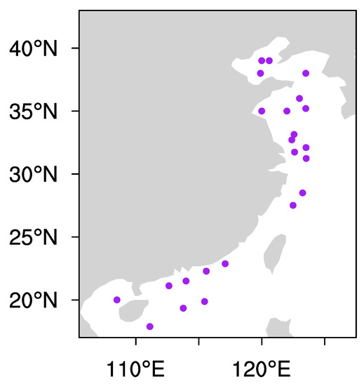
Figure 1.
Positions of the buoys in China’s offshore waters, where purple dots indicate the buoys‘ location.
2.3. HY−2B SWH Data
HY−2B is the second (after HY−2A) Chinese radar altimeter [44]. This is the marine dynamic−environment satellite launched by China on 25 October 2018 [45]. It has a dual−frequency radar operating in the 13.58 GHz (Ku) and 5.25 GHz (C) bands [34]. Geophysical data records were obtained from the NSOAS data service website (< https://osdds.nsoas.org.cn> [last accessed on 31 January 2023]). The ground processing of data utilizes the MLE4 (Maximum Likelihood Estimator) retracking algorithm inherited from the HY−2A altimeter [40,46]. The data quality of HY−2B is high and basically the same as that of an international−radar altimeter such as the Jason−3 satellite [34]. The RMSE of HY−2B SWH against NDBC buoys and Jason−3 are 0.27 m and 0.30 m, respectively [31]. Both HY−2B and CFOSAT were launched in October 2018. Since these two satellites have similar on−orbit periods, there were many matched SWHs available for studying the accuracy differences between the CFOSAT SWIM and HY−2B satellite radar altimeter.
According to the validation details for both the HY−2B Ku−band and C−band SWH by Jia et al. [34] and Li et al. [31], the Ku−band SWH shows better performance than the one from the C band. The HY−2B Ku−band for SWH was selected, from which the best data, particularly those unaffected by precipitation, were selected using a set of various criteria and parameter thresholds from the SWH data, such as quality flags. For example, “rain_flag”, “ice_flag”, and “qual_alt_1 hz_swh_ku_j3” were all selected to be “0” for the data used in the analysis.
2.4. Methods
In the comparison of the CFOSAT SWH against the HY−2B SWH, to minimize the impacts of sea ice, the collocated SWH data were confined to the region between 60°S and 60°N [34], with temporal and spatial windows of 30 min and 50 km, respectively. The comparison of the SWH from CFOSAT against in−situ−buoy SWH data also used the same temporal and spatial windows. To replicate the seasonal differences between the CFOSAT and HY−2B SWH in complete seasons, the data from December 2019 to November 2021 were used.
Up to 23 buoy measurements that had overlapping measurement periods with the satellites for 28 months were analyzed in detail. To obtain the monthly variance of the statistical parameters of CFOSAT SWH against the buoy observations, the statistical parameters of matched SWHs in every month were calculated. Referring to the validation method [47], the statistical parameters used included the relative absolute error (RAE), scattering index (SI), correlation coefficient (R), RMSE, and temporal standard deviation for every grid box (Tstd), defined as follows:
where is the SWH from CFOSAT, is the SWH observation from the buoy, is the number of matched data pairs, in Equation (5) x is the SWH in one grid box from CFOSAT or HY−2B, and n is the number−of−times series in the grid box.
The research area of this study covered China’s offshore waters (0°–45°N, 105°–127°E). The four seasons analyzed were boreal winter, defined as December–January–February (DJF), spring, defined as March–April–May (MAM), summer, defined as June–July–August (JJA), and autumn, defined as September–October–November (SON). Taking different sea conditions into account [37], an SWH of around 1.25 m denotes calm sea conditions, and an SWH of over 5 m denotes rough sea conditions.
3. Results
3.1. Validation of CFOSAT with In Situ SWH
In order to validate the CFOSAT SWH in China’s offshore waters, we collected observations from 23 buoys (Figure 1), which covered almost the entire coastline of China. The scatter−point density plot of CFOSAT versus the 23 buoys in 28 months, which contains 21,049 matched SWHs, revealed the overall accuracy of the CFOSAT SWH (Figure 2a). The SI and RMSE of the CFOSAT nadir SWH were 20% and 0.29 m, respectively. The RMSE was larger than the value (0.21 m) from the NDBC buoys [20]. According to Figure 2a, CFOSAT SWHs showed a close relationship with buoy observations with a correlation coefficient of 0.96. Higher densities of matched points in the range < 2 m were observed, with most of the matched points located near the diagonal line. In some cases, observed low SWHs (less than 0.5 m) matched the high CFOSAT SWHs (greater than 1 m). CFOSAT tends to overestimate the SWH in the range of <2 m, especially in the range of <1.25 m, where the relative bias was approximately 20–40% (Figure 2b). Also, the highest accuracy was observed for an SWH of around 4–4.5 m. This means that the relative absolute error was greater under calm sea conditions (defined in Section 2.4) than under rough sea conditions. A similar result has also been reported using National Data Buoy Center buoys [31].
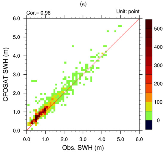
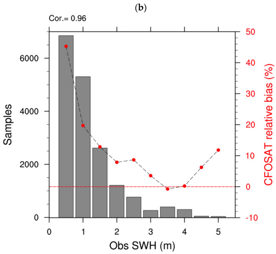
Figure 2.
Scatter−point density plot of the CFOSAT SWH versus that of 23 buoys (a) and the relative bias according to the SWH of buoys in intervals of 0.5 m with samples numbers, where red dots indicate the relative bias of CFOSAT SWH against observation (b). The temporal and spatial windows are 30 min and 50 km, respectively, and 21,049 matched SWHs were used.
The variability of the combined RAE showed a seasonal cycle (Figure 3a, red line); however, it varied in a narrow range near 35%. The linear−correction equation can be used to correct the CFOSAT SWHs in China’s offshore waters. This variation has a connection with the sea−surface wind from the buoy observations (Figure 3b, pink line), which also exhibited a seasonal cycle. Generally, in spring and summer when weaker sea−surface winds and SWHs appear (Figure 3b, green line), the RAE is greater when compared with that in autumn and winter. When the sea−surface wind is relatively low (Figure 3b, pink line), calm sea conditions occur. Under these calm sea conditions, CFOSAT tends to overestimate the SWH compared with that in other SWH ranges.
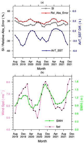
Figure 3.
The variance of RAE and SI of CFOSAT SWH with in situ observations (a), where the RAE (red line) is defined in Section 2.4. The temporal and spatial windows are set to 30 min and 50 km, respectively. The RAEs of 23 buoys were used to calculate the monthly mean. The air−temperature and sea−surface−temperature differences (blue line) have a significant correlation with the RAE at the 95% confidence level as observed in (a) but for variance of sea−surface wind speed and SWH (b). The temporal−correlation coefficient between the SWH from the buoys ((b), green line) and the monthly mean RAE is −0.73 (statistically significant at the 95% confidence level). The Scatter Index ((a), gray line) and wind speed from the buoys ((b), pink line) are the monthly mean of 23 buoys in a month.
Usually, from October to May, temperature inversions appear mostly in the air–sea interface layer along the southeastern coast of China, in the west and south of the Korean Peninsula, and in the north and east of the Shandong Peninsula [48]. It is worth noting that the RAEs were also relatively low in some high sea−surface wind−speed months. During this period, a relatively low SWH appeared (Figure 3b, green line). The air–sea temperature difference played a key role in the sea−surface roughness [49], especially in April 2020 and May 2021. Also, the seasonal variance of air–sea temperature inversion had an influence on the RAE.
According to previous results comparing CFOSAT against the Jason−3 altimeter SWH [20,31], CFOSAT seems to overestimate the SWH under calm sea conditions as well. In East Asia, calm sea conditions usually occur in spring and summer, whereas rough sea conditions occur in winter, which plays a crucial role in the RAE seasonal cycle.
3.2. Evaluation of HY−2B Performance with In Situ SWH
In order to evaluate the performance of HY−2B in China’s offshore waters, we used the same temporal and spatial windows and eliminated the buoys within 25 km of the coastline (details in Section 2.2). For a broader coverage, more matched SWHs collected in the same time period, including 24,896 samples from 30 buoys, were analyzed than the SWHs for CFOSAT (Figure 4). These buoy locations cover most of the China’s offshore waters and some open−sea waters (e.g., in the central South China Sea).
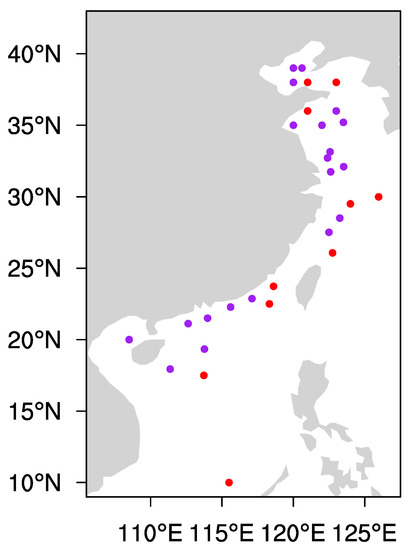
Figure 4.
As in Figure 1, but for the HY−2B matched buoy positions. The purple dots indicate the marched SWHs from the buoys that also have matched SWHs with CFOSAT, and the red dots indicate the matched SWHs from the buoys that only have matched SWHs with HY−2B (30 buoys in total).
The matched scatter−point density shows a linear correlation between HY−2B and in situ SWHs (Figure 5a), where most HY−2B SWHs were greater than observed. The RMSE was 0.34 m higher than from CFOSAT but lower than the value (0.38 m) against the NDBC buoys [50]. Based on the relative bias in each 0.5 m range, HY−2B tended to overestimate the SWH below 2 m, especially in the range of <1.25 m, which is similar to the CFOSAT result. HY−2B tended to underestimate the SWH at around 5 m. In the range of >2 m, HY−2B showed relatively high−quality SWHs, where the relative bias was about 10% (Figure 5b). Linear correction can be used as a preliminary step to correct the HY−2B SWHs.
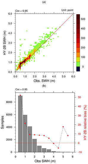
Figure 5.
As in Figure 2, but for the SWH of HY−2B compared to that of 30 buoys, where red dots indicate the relative bias of HY−2B SWH against observation and 24,896 matched SWHs were used.
Comparing the CFOSAT and HY−2B in−situ−validation results, CFOSAT and HY−2B both showed a close relationship according to observations made. CFOSAT and HY−2B tended to overestimate the SWHs in the range of <2 m; moreover, HY−2B probably overestimated the SWH in the range of <1.25 m more than CFOSAT. CFOSAT showed a relative advantage in the SWH range of 3.5–4.5 m.
Generally, despite the sensors onboard CFOSAT and HY−2B being different, their SWH results showed high correlation with observations. Linear−correlation equations can be used as a preliminary step to correct the SWH from both CFOSAT and HY−2B.
3.3. Comparison of CFOSAT and HY−2B SWHs Variation
The spatial coverage of SWH played a key role in evaluating the time scale on which to establish a gridded satellite dataset. We split the area into 25 km × 25 km grid boxes (the same as the horizontal resolution of the original swaths [51]) and calculated the cumulative number of boxes in which there was at least one data point, for 1 to 31 days (Figure 6). The overlapping boxes were considered only once, even if there were two or more measurements located in the box.
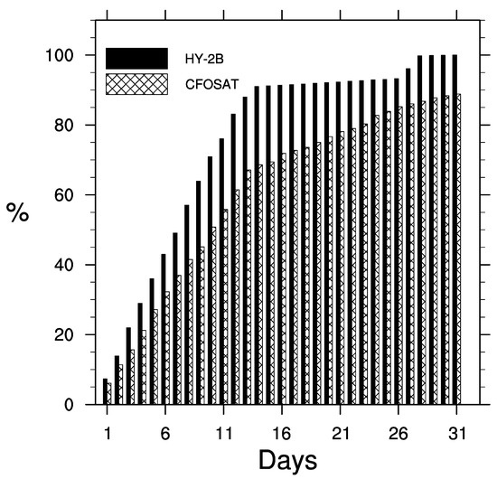
Figure 6.
The coverage variance according to the number of days. The solid, filled bars indicate the coverage of HY−2B over East Asia, while the cross−hatched bars denote the coverage variance of CFOSAT according to the number of days. The 31−day cumulative box of HY−2B is set as 100%.
According to the daily increment of spatial coverage of the CFOSAT SWH (Figure 6), one month can be divided into two stages: a rapidly increasing stage and a relatively stable stage. The rapid daily−increment stage was between 1 and 12 days. The period after 13 days was the relatively stable stage, and the coverage increased slowly with time.
In contrast, according to the daily increment of spatial coverage of HY−2B, one month can be classified into three stages. A rapid daily−increasing stage occurred from 1 to 13 days, a slow daily−increasing stage occurred from 14 to 27 days, and a stable stage occurred after 28 days, when the coverage of HY−2B reached its maximum.
Owing to the design of the satellite orbit, the coverage of HY−2B was greater than that of CFOSAT. HY−2B also had a greater geographic coverage than that of Jason−3 [34]. Weighting the spatial coverage and time scale of the final gridded SWHs, we found that a 10−day mean was a relatively reasonable time scale for interpolating CFOSAT and HY−2B nadir swath SWHs into gridded boxes with a horizontal resolution of 25 km × 25 km.
To validate the spatial distribution of SWHs in a complete season, especially in winter, the HY−2B and CFOSAT seasonal mean SWHs were used for the corresponding period from December 2019 to November 2021 (Figure 7). The nadir SWHs were corrected with observations (equations listed in Table 1) and then interpolated into a 25 km × 25 km grid using the Cressman analysis, which is usually applied to interpolate meteorological station observations [52].
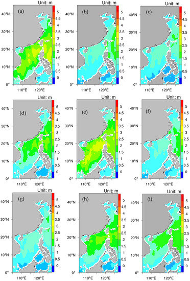
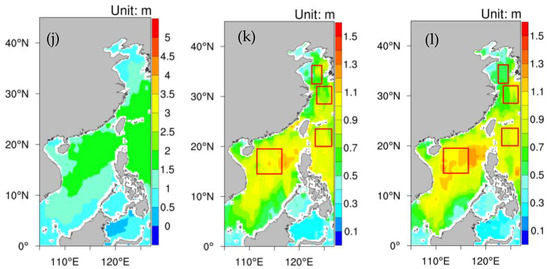
Figure 7.
Seasonal mean SWH for CFOSAT and HY−2B from December 2019 to November 2021. The seasonal mean in DJF (a), MAM (b), JJA (c), and SON (d), and the annual mean (i) and standard deviation (k), respectively. (e–h,j,l) As in (a–d,i,k) but for HY−2B. The red boxes in (k) and (l), from north to south, indicate 4 sea areas of concern in Huanghai, Donghai, East Taiwan, and the central South China Sea, respectively.

Table 1.
Seasonal field mean SWH and correct equations.
Figure 5 and Figure 7a illustrate that, for a typical winter−monsoon season in East Asia (DJF), the SWH distribution from CFOSAT is similar to that from HY−2B in East Asia, with a field correlation coefficient of 0.97 in DJF. In contrast, the lowest field correlation coefficient of 0.92 occurs in spring. The SWH from CFOSAT was greater than that from HY−2B in China’s offshore waters. Considering the SWH distribution in the Taiwan Strait, CFOSAT showed more feasible results compared with HY−2B. The DJF field mean of SWH was 1.8 m for CFOSAT, which is the same as the SWH for HY−2B (summarized in Table 1).
In boreal spring (MAM) in East Asia, the spatial distributions of the seasonal mean SWH from CFOSAT and HY−2B showed less similarity than in winter, with a field−correlation coefficient of 0.92 (Figure 7b,f). During this seasonal−transition period, the weakened mean flow causes a moderate surface wind in spring, which forms calm sea conditions. Based on the in−situ−validation results, CFOSAT has a lower accuracy than in winter. The field mean SWH was 0.9 m for CFOSAT and 1.0 m for HY−2B.
In boreal summer (JJA, Figure 7c,g), the spatial distributions of the seasonal mean SWH from CFOSAT and HY−2B were more uniform compared with in spring, with a field correlation coefficient of 0.94. The CFOSAT SWH in the waters near the coastline accords well with that from HY−2B, but not for the open sea waters, especially to the northeast of Taiwan Island, which weakens the field correlation coefficient.
In autumn (SON), the SWH distribution was uniform between CFOSAT and HY−2B, with a field correlation coefficient of 0.97, especially in the South China Sea (Figure 7d,h). The CFOSAT field mean SWH was the same as the HY−2B SWH at 1.3 m.
To further summarize the comparison between CFOSAT and HY−2B, we analyzed the annual mean SWH (Figure 7i,j), which revealed a field correlation coefficient of 0.98, thereby, indicating that the spatial variation of SWH was quite similar between CFOSAT and HY−2B. The field means of the annual SWH from CFOSAT and HY−2B were the same, with a mean SWH of 1.2 m for CFOSAT, which was the same as that for HY−2B. The monthly mean SWHs of CFOSAT and HY−2B showed an obviously similar seasonal cycle, with the highest value in winter and the lowest value in summer. In spring, the field correlation coefficient was the lowest among the four seasons, which indicates that in the period of low sea−surface winds and apparent air–sea temperature inversion, the differences between CFOSAT and HY−2B were greater.
The standard deviation based on the time series of every 10−day mean SWH from 2020 to 2021 showed a variation in SWH magnitude throughout the study period (Figure 7k,l). The spatial distribution of the CFOSAT SWH standard deviation was similar to that of HY−2B, with a field correlation coefficient of 0.87. The SWH from CFOSAT and HY−2B shared a fairly uniform spatial distribution in terms of their variation in magnitude in China’s offshore waters among the four seasons.
Figure 8 shows the characteristics of the variation in SWH between HY−2B and CFOSAT for every 10−day mean series from December 2019 to December 2021 in the four sea areas of concern (Figure 8a–d). During the study period, the variations of SWH from CFOSAT and HY−2B showed a close relationship (Figure 8a–d), with most of the sea areas having statistically significant correlation coefficients at the 95% confidence level.
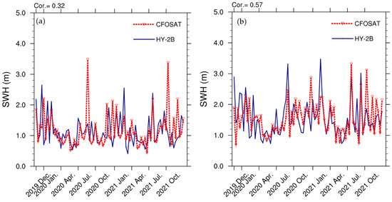
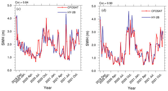
Figure 8.
Field mean SWH variance from HY−2B (blue line) and CFOSAT (red line) for every 10−day mean series from December 2019 to December 2021 (78 time series in total). The selected waters are shown in Figure 7k,l (red boxes). The boxes, from north to south, are Huanghai (a), Donghai (b), east of Taiwan (c), and the central South China Sea (d), respectively.
Among the four sea areas, it was interesting to find that the correlation coefficient increased with SWH magnitude. Compared with HY−2B, more extreme high SWHs occurred in northern waters according to CFOSAT, such as in October in Huanghai (Figure 8a), leading to a smaller correlation coefficient. The CFOSAT SWHs varied uniformly with HY−2B to the east of Taiwan (Figure 8c) and in the central South China Sea (Figure 8d).
An intercomparison of CFOSAT and HY−2B data over a larger domain with over 170,000 points was carried out between 60°S and 60°N (Figure 9a), with the criteria of a spatial window of 50 km and a time window of 30 min [34]. There were three peak zones of a total number of zonal points: one near the equator and the other two near the midlatitude in the northern hemisphere and southern hemisphere. The SWHs from CFOSAT were consistent with those from HY−2B in all SWH ranges, with a correlation coefficient of 0.99 (Figure 9b), which agrees with the findings of Li et al. [31]. It is worth noting that, in calm sea conditions (SWH < 1.25 m), CFOSAT and HY−2B both tended to overestimate the SWH. Similar results were also found in the CFOSAT SWH validation against buoy observations in summer (relatively calm sea conditions) in Section 3.1 and Section 3.2.
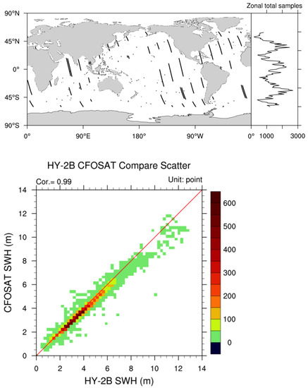
Figure 9.
Locations of matched points between HY−2B and CFOSAT nadir measurements and zonal total samples at every latitude (top), and a scatter−point density plot of HY−2B versus CFOSAT SWH (bottom). The data were selected with a 50 km spatial window and 30 min time window between CFOSAT and HY−2B observations between 60°S and 60°N.
4. Conclusions
In East Asia, a typical monsoon−affected area, the sea−surface wind speed varies considerably in magnitude between summer and winter. This different seasonal mean flow can directly lead not only to variations in SWH but also to the appearance of air–sea temperature inversion. This issue cannot be simply eliminated by setting up some flag (e.g., a rain detection flag or an ice flag). However, there have been limited, in situ validations of SWHs performed in these waters with such complex sea conditions. In this study, we validated the SWHs from CFOSAT against in situ buoy observations for China’s offshore waters from July 2019 to December 2021 with temporal and spatial windows of 30 min and 50 km, respectively. The SI and RMSE of the CFOSAT nadir SWH were 20% and 0.29 m, respectively. The main findings of our study can be summarized as follows:
- (1)
- On the basis of 23 in situ buoy observations in China’s offshore waters, CFOSAT tends to overestimate the SWH in the range of <2 m, especially in the range of <1.25 m, where the relative bias is about 20–40%. The highest point of accuracy is observed for the SWH in the range of around 4–4.5 m. The SI and RMSE of the CFOSAT nadir SWH are 20% and 0.29 m, respectively. The RAE shows an obvious seasonal cycle, varying in a narrow range near 35%. A linear−correction equation can be used to correct the CFOSAT SWHs in China’s offshore waters. The sea condition plays a crucial role in the RAE seasonal cycle, which is influenced by the sea−surface wind speed and air–sea temperature inversion. Both are controlled by seasonal mean flow.
- (2)
- Weighting the spatial coverage and time interval of the final gridded SWHs, a 10−day mean was used for interpolating CFOSAT and HY−2B swath SWHs into grid boxes. A comparison of the corrected CFOSAT grid−box SWH against that of HY−2B showed that the spatial distribution of SWH agreed well with that from HY−2B in the four seasons, with a field correlation coefficient exceeding 0.98 for two years of mean SWHs. In winter, when the SWH is greater, the field correlation coefficient is 0.97, as compared to spring, when the field correlation coefficient is 0.92.
- (3)
- Among four selected sea areas, the field mean SWH variance of CFOSAT and HY−2B showed a close relationship. Moreover, the correlation coefficient of the field mean SWH variance from CFOSAT and HY−2B increased with the mean SWH magnitude. Compared with HY−2B, more extremely high CFOSAT SWHs occurred in the Huanghai seawater area.
- (4)
- For a broader coverage of HY−2B than CFOSAT, 24,896 matched SWHs from 30 buoys were found in almost the entire region of China’s offshore waters. The validation results indicated that, normally, the HY−2B SWH is higher than observed, with an RMSE of 0.34, which is greater than that of CFOSAT. The SWH of both CFOSAT and HY−2B shared a close relationship with the observed data, in which the HY−2B SWH showed a greater overestimation than CFOSAT in the SWH range of <1.25 m. Scatter−point density plots of CFOSAT and HY−2B SWHs versus buoy data suggest that linear correlation equations can be applied as a preliminary step to correct the SWHs of both satellites.
- (5)
- The matched points from the intercomparison of CFOSAT and HY−2B SWHs were distributed evenly over the latitudes. These SWHs from CFOSAT were consistent with those from HY−2B in all SWH ranges. In calm sea conditions (SWH < 1.25 m), both CFOSAT and HY−2B tend to overestimate the SWH.
To maintain a clear focus in this study, we concentrated on the validation of CFOSAT SWHs and the characteristics of their variance in China’s offshore waters. Nevertheless, other factors, such as the sandy intertidal zone [53,54,55,56] and ocean swell [57,58,59,60], can influence the results. Despite the limited number of observations, consisting of 23 buoys moored in China’s offshore waters, and the period of overlap (two years) with HY−2B SWH data, the results show that the sea conditions have a strong connection with the RAE seasonal cycle. This study emphasizes that, in such special seasonal mean−flow−affected waters, especially in the mid−latitude offshore waters of China, attention should be given to the adverse effects of the sea conditions on the accuracy of CFOSAT SWH. Furthermore, more validation results with in−situ observations from China’s offshore waters and the mechanism behind the seasonal mean flow and SWH accuracy are worthy of investigation in the future.
Author Contributions
J.X. initiated and coordinated the work. J.X. and M.X. provided the calculation and validation. J.X., N.V.K., Y.X. and M.X. wrote the manuscript. H.W., X.Z. (Xiuzhi Zhang), L.K. and K.F. gave valuable suggestions for revisions. X.Z. (Xiefei Zhi) revised the analysis. All authors have read and agreed to the published version of the manuscript.
Funding
This research was jointly supported by the National Natural Science Foundation of China (Grant No. 42275164) entitled “Research on 8−42d Subseasonal Multi-mode Integrated Forecasting Based on Statistical Methods and Machine Learning”, the key project of the Ministry of Science and Technology of China (Grant No. SQ2022AAA010127), the Fengyun satellite application advance plan from China Meteorological Administration (Grant No. FY-APP-2021.0304). This study was also funded by “the Priority Academic Program Development of Jiangsu Higher Education Institutions” (PAPD).
Data Availability Statement
The datasets generated for this study are available on request to the corresponding author.
Acknowledgments
We thank anonymous reviewers for comments and suggestions that helped to improve the manuscript. Also, we thank CNES and NSOAS for providing the CFOSAT data, NSOAS for providing the HY−2B data, and SOAC for providing the buoy observations.
Conflicts of Interest
The authors declare no conflict of interest.
References
- Xu, J.; Koldunov, N.; Remedio, A.R.C.; Sein, D.V.; Zhi, X.; Jiang, X.; Xu, M.; Zhu, X.; Fraedrich, K.; Jacob, D.J.C.d. On the role of horizontal resolution over the Tibetan Plateau in the REMO regional climate model. Clim. Dyn. 2019, 51, 4525–4542. [Google Scholar] [CrossRef]
- Xu, J.; Koldunov, N.V.; Remedio, A.R.C.; Sein, D.V.; Rechid, D.; Zhi, X.; Jiang, X.; Xu, M.; Zhu, X.; Fraedrich, K.; et al. Downstream effect of Hengduan Mountains on East China in the REMO regional climate model. Theor. Appl. Climatol. 2018, 135, 1641–1658. [Google Scholar] [CrossRef]
- Timmermans, B.W.; Gommenginger, C.P.; Dodet, G.; Bidlot, J.R. Global Wave Height Trends and Variability from New Multimission Satellite Altimeter Products, Reanalyses, and Wave Buoys. Geophys. Res. Lett. 2020, 47, 9. [Google Scholar] [CrossRef]
- Dobson, E.; Monaldo, F.; Goldhirsh, J.; Wilkerson, J. Validation of Geosat altimeter-derived wind speeds and significant wave heights using buoy data. J. Geophys. Res. Ocean. 1987, 92, 10719–10731. [Google Scholar] [CrossRef]
- Kettle, A.J. A diagram of wind speed versus air-sea temperature difference to understand the marine atmospheric boundary layer. Energy Procedia 2015, 76, 138–147. [Google Scholar] [CrossRef]
- Sun, M.; Du, J.; Yang, Y.; Yin, X. Evaluation of Assimilation in the MASNUM Wave Model Based on Jason-3 and CFOSAT. Remote Sens. 2021, 13, 3833. [Google Scholar] [CrossRef]
- Zhi, X.; Pan, M.; Song, B.; Wang, J. Investigating air-sea interactions in the North Pacific on interannual timescales during boreal winter. Atmos. Res. 2022, 269, 106043. [Google Scholar] [CrossRef]
- Durrant, T.H.; Greenslade, D.J.; Simmonds, I. Validation of Jason-1 and Envisat remotely sensed wave heights. J. Atmos. Ocean. Technol. 2009, 26, 123–134. [Google Scholar] [CrossRef]
- Koldunov, N.V.; Danilov, S.; Sidorenko, D.; Hutter, N.; Losch, M.; Goessling, H.; Rakowsky, N.; Scholz, P.; Sein, D.; Wang, Q. Fast EVP solutions in a high-resolution sea ice model. J. Adv. Model. Earth Syst. 2019, 11, 1269–1284. [Google Scholar] [CrossRef]
- Toledano, C.; Ghantous, M.; Lorente, P.; Dalphinet, A.; Aouf, L.; Sotillo, M.G. Impacts of an Altimetric Wave Data Assimilation Scheme and Currents-Wave Coupling in an Operational Wave System: The New Copernicus Marine IBI Wave Forecast Service. J. Mar. Sci. Eng. 2022, 10, 457. [Google Scholar] [CrossRef]
- Shao, W.; Jiang, T.; Zhang, Y.; Shi, J.; Wang, W. Cyclonic Wave Simulations Based on WAVEWATCH-III Using a Sea Surface Drag Coefficient Derived from CFOSAT SWIM Data. Atmosphere 2021, 12, 1610. [Google Scholar] [CrossRef]
- Donlon, C.; Berruti, B.; Buongiorno, A.; Ferreira, M.-H.; Féménias, P.; Frerick, J.; Goryl, P.; Klein, U.; Laur, H.; Mavrocordatos, C. The global monitoring for environment and security (GMES) sentinel-3 mission. Remote Sens. Environ. 2012, 120, 37–57. [Google Scholar] [CrossRef]
- Ribal, A.; Young, I.R. 33 years of globally calibrated wave height and wind speed data based on altimeter observations. Sci. Data 2019, 6, 77. [Google Scholar] [CrossRef]
- Jin, S.; Yang, S.; Yan, Q.; Jia, Y. Significant wave height estimation from CYGNSS delay-doppler map average observations. In Proceedings of the 2022 Photonics & Electromagnetics Research Symposium (PIERS), Hangzhou, China, 25–29 April 2022. [Google Scholar]
- Ren, L.; Yang, J.; Xiao, Q.; Zheng, G.; Wang, J. On CFOSAT swim wave spectrometer retrieval of ocean waves. In Proceedings of the 2017 IEEE International Geoscience and Remote Sensing Symposium (IGARSS), Fort Worth, TX, USA, 23–28 July 2017. [Google Scholar]
- Xiang, K.; Yin, X.; Xing, S.; Kong, F.; Li, Y.; Lang, S.; Gao, Z. Preliminary Estimate of CFOSAT Satellite Products in Tropical Cyclones. IEEE Trans. Geosci. Remote Sens. 2022, 60, 1–16. [Google Scholar] [CrossRef]
- Aouf, L.; Dalphinet, A.; Hauser, D.; Delaye, L.; Tison, C.; Chapron, B.; Hermozo, L.; Tourain, C. On the Assimilation of CFOSAT Wave Data in the Wave Model MFWAM: Verification Phase. In Proceedings of the IGARSS 2019—2019 IEEE International Geoscience and Remote Sensing Symposium, Yokohama, Japan, 28 July–2 August 2019. [Google Scholar]
- Hauser, D.; Tourain, C.L.; Hermozo, L.; Alraddawi, D.; Aouf, L.; Chapron, B.; Dalphinet, A.; Delaye, L.; Dalila, M.; Dormy, E.; et al. New Observations from the SWIM Radar On-Board CFOSAT: Instrument Validation and Ocean Wave Measurement Assessment. IEEE Trans. Geosci. Remote Sens. 2020, 59, 5–26. [Google Scholar] [CrossRef]
- Liu, J.; Lin, W.; Dong, X.; Lang, S.; Yun, R.; Zhu, D.; Zhang, K.; Sun, C.; Mu, B.; Ma, J.; et al. First Results from the Rotating Fan Beam Scatterometer Onboard CFOSAT. IEEE Trans. Geosci. Remote Sens. 2020, 58, 8793–8806. [Google Scholar] [CrossRef]
- Xu, Y.; Liu, J.; Xie, L.; Sun, C.; Liu, J.; Li, J.; Xian, D. China-France Oceanography Satellite (CFOSAT) simultaneously observes the typhoon-induced wind and wave fields. Acta Oceanol. Sin. 2019, 38, 158–161. [Google Scholar] [CrossRef]
- Tang, S.; Chu, X.; Jia, Y.; Li, J.; Liu, Y.; Chen, Q.; Li, B.; Liu, J.; Chen, W. An Appraisal of CFOSAT Wave Spectrometer Products in the South China Sea. Earth Space Sci. 2022, 9. [Google Scholar] [CrossRef]
- Wang, J.K.; Aouf, L.; Dalphinet, A.; Zhang, Y.; Xu, Y.; Hauser, D.; Liu, J.Q. The Wide Swath Significant Wave Height: An Innovative Reconstruction of Significant Wave Heights from CFOSAT’s SWIM and Scatterometer Using Deep Learning. Geophys. Res. Lett. 2021, 6, 48. [Google Scholar] [CrossRef]
- Ren, L.; Yang, J.; Xu, Y.; Zhang, Y.; Zheng, G.; Wang, J.; Dai, J.; Jiang, C.L. Ocean Surface Wind Speed Dependence and Retrieval from Off-Nadir CFOSAT SWIM Data. Earth Space Sci. 2021, 8. [Google Scholar] [CrossRef]
- Freilich, M.H.; Dunbar, R.S. The accuracy of the NSCAT 1 vector winds: Comparisons with National Data Buoy Center buoys. J. Geophys. Res. 1999, 104, 11231–11246. [Google Scholar] [CrossRef]
- Meindl, E.A.; Hamilton, G.D. Programs of the National Data Buoy Center. Bull. Am. Meteorol. Soc. 1992, 73, 985–993. [Google Scholar] [CrossRef]
- Hamilton, G.D. National Data Buoy Center Programs. Bull. Am. Meteorol. Soc. 1986, 67, 411–415. [Google Scholar] [CrossRef]
- Teng, C.-c.; Cucullu, S.; McArthur, S.; Kohler, C.; Burnett, B.; Bernard, L. Buoy vandalism experienced by NOAA National Data Buoy Center. OCEANS 2009, 2009, 1–8. [Google Scholar]
- Hall, C.; Jensen, R.E. Utilizing Data from the NOAA National Data Buoy Center; Coastal and Hydraulics Laboratory: Vicksburg, MS, USA, 2021. [Google Scholar]
- Liang, G.; Yang, J.; Wang, J. Accuracy Evaluation of CFOSAT SWIM L2 Products Based on NDBC Buoy and Jason-3 Altimeter Data. Remote Sens. 2021, 13, 887. [Google Scholar] [CrossRef]
- Li, B.; Li, J.; Liu, J.; Tang, S.; Chen, W.; Shi, P.; Liu, Y. Calibration Experiments of CFOSAT Wavelength in the Southern South China Sea by Artificial Neural Networks. Remote Sens. 2022, 14, 773. [Google Scholar] [CrossRef]
- Li, X.; Xu, Y.; Liu, B.; Lin, W.; He, Y.; Liu, J. Validation and Calibration of Nadir SWH Products from CFOSAT and HY-2B With Satellites and In Situ Observations. J. Geophys. Res. Ocean. 2021, 126, e2020JC016689. [Google Scholar] [CrossRef]
- Quartly, G.D.; Chen, G.; Nencioli, F.; Morrow, R.; Picot, N. An Overview of Requirements, Procedures and Current Advances in the Calibration/Validation of Radar Altimeters. Remote Sens. 2021, 13, 125. [Google Scholar] [CrossRef]
- Zou, J.; Lin, M.; Zou, B.; Guo, M.; Cui, S. Fusion of sea surface wind vector data acquired by multi-source active and passive sensors in China sea. Int. J. Remote Sens. 2017, 38, 6477–6491. [Google Scholar] [CrossRef]
- Jia, Y.; Yang, J.; Lin, M.; Zhang, Y.; Ma, C.; Fan, C. Global assessments of the HY-2B measurements and cross-calibrations with Jason-3. Remote Sens. 2020, 12, 2470. [Google Scholar] [CrossRef]
- Dodet, G.; Piolle, J.-F.; Quilfen, Y.; Abdalla, S.; Accensi, M.; Ardhuin, F.; Ash, E.; Bidlot, J.-R.; Gommenginger, C.; Marechal, G. The Sea State CCI dataset v1: Towards a sea state climate data record based on satellite observations. Earth Syst. Sci. Data 2020, 12, 1929–1951. [Google Scholar] [CrossRef]
- Young, I.R.; Vinoth, J.; Zieger, S. Joint Calibration of Multiplatform Altimeter Measurements of Wind Speed and Wave Height over the Past 20 Years. J. Atmos. Ocean. Technol. 2009, 26, 2549–2564. [Google Scholar] [CrossRef]
- Xu, Y.; Hauser, D.; Liu, J.; Si, J.; Yan, C.; Chen, S.; Meng, J.; Fan, C.; Liu, M.; Chen, P. Statistical Comparison of Ocean Wave Directional Spectra Derived From SWIM/CFOSAT Satellite Observations and From Buoy Observations. IEEE Trans. Geosci. Remote Sens. 2022, 60, 1–20. [Google Scholar] [CrossRef]
- Jiang, H.; Mironov, A.; Ren, L.; Babanin, A.V.; Wang, J.; Mu, L. Validation of Wave Spectral Partitions from SWIM Instrument On-Board CFOSAT Against In Situ Data. IEEE Trans. Geosci. Remote Sens. 2022, 60, 1–13. [Google Scholar] [CrossRef]
- Hauser, D.; Tison, C.; Amiot, T.; Delaye, L.; Corcoral, N.; Castillan, P. SWIM: The First Spaceborne Wave Scatterometer. IEEE Trans. Geosci. Remote Sens. 2017, 55, 3000–3014. [Google Scholar] [CrossRef]
- Yang, J.; Zhang, J.; Jia, Y.; Fan, C.; Cui, W. Validation of Sentinel-3A/3B and Jason-3 Altimeter Wind Speeds and Significant Wave Heights Using Buoy and ASCAT Data. Remote Sens. 2020, 12, 2079. [Google Scholar] [CrossRef]
- Tran, N.; Vandemark, D.; Zaron, E.D.; Thibaut, P.; Dibarboure, G.; Picot, N. Assessing the effects of sea-state related errors on the precision of high-rate Jason-3 altimeter sea level data. Adv. Space Res. 2021, 68, 963–977. [Google Scholar] [CrossRef]
- Han, L.; Ji, Q.; Jia, X.; Liu, Y.; Han, G.; Lin, X. Significant Wave Height Prediction in the South China Sea Based on the ConvLSTM Algorithm. J. Mar. Sci. Eng. 2022, 10, 1683. [Google Scholar] [CrossRef]
- Zhang, K.; Dong, X.; Zhu, D.; Yun, R. Estimation and Correction of Geolocation Errors of the CFOSAT Scatterometer Using Coastline Backscatter Coefficients. IEEE J. Sel. Top. Appl. Earth Obs. Remote Sens. 2021, 14, 53–61. [Google Scholar] [CrossRef]
- Tourain, C.; Piras, F.; Ollivier, A.; Hauser, D.; Poisson, J.C.; Boy, F.; Thibaut, P.; Hermozo, L.; Tison, C. Benefits of the Adaptive Algorithm for Retracking Altimeter Nadir Echoes: Results from Simulations and CFOSAT/SWIM Observations. IEEE Trans. Geosci. Remote Sens. 2021, 59, 9927–9940. [Google Scholar] [CrossRef]
- Wang, J.; Aouf, L.; Jia, Y.; Zhang, Y. Validation and Calibration of Significant Wave Height and Wind Speed Retrievals from HY2B Altimeter Based on Deep Learning. Remote Sens. 2020, 12, 2858. [Google Scholar] [CrossRef]
- Xu, X.-Y.; Xu, K.; Shen, H.; Liu, Y.-L.; Liu, H.-G. Sea Surface Height and Significant Wave Height Calibration Methodology by a GNSS Buoy Campaign for HY-2A Altimeter. IEEE J. Sel. Top. Appl. Earth Obs. Remote Sens. 2016, 9, 5252–5261. [Google Scholar] [CrossRef]
- Yang, J.; Zhang, J. Validation of Sentinel-3A/3B satellite altimetry wave heights with buoy and Jason-3 data. Sensors 2019, 19, 2914. [Google Scholar] [CrossRef] [PubMed]
- Hao, J.; Chen, Y.; Wang, F. Temperature inversion in China seas. J. Geophys. Res. Ocean. 2010, 115. [Google Scholar] [CrossRef]
- Shi, Q.; Bourassa, M.A. Coupling Ocean Currents and Waves with Wind Stress over the Gulf Stream. Remote Sens. 2019, 11, 1476. [Google Scholar] [CrossRef]
- Ye, X.; Lin, M.; Xu, Y. Validation of Chinese HY-2 satellite radar altimeter significant wave height. Acta Oceanol. Sin. 2015, 34, 60–67. [Google Scholar] [CrossRef]
- Yun, R.; Dong, X.; Liu, J.; Lin, W.; Zhu, D.; Ma, J.; Lang, S.; Wang, Z. CFOSAT Rotating Fan-Beam Scatterometer Backscatter Measurement Processing. Earth Space Sci. 2021, 8, 11. [Google Scholar] [CrossRef]
- Cressman, G.P. An Operational Objective Analysis System. Mon. Weather. Rev. 1959, 87, 367–374. [Google Scholar] [CrossRef]
- Ram, K.R.; Narayan, S.; Ahmed, M.R.; Nakavulevu, P.; Lee, Y.-H. In situ near-shore wave resource assessment in the Fiji Islands. Energy Sustain. Dev. 2014, 23, 170–178. [Google Scholar] [CrossRef]
- Befus, K.M.; Cardenas, M.B.; Erler, D.V.; Santos, I.R.; Eyre, B.D. Heat transport dynamics at a sandy intertidal zone. Water Resour. Res. 2013, 49, 3770–3786. [Google Scholar] [CrossRef]
- Li, Y.; Chen, W.; Cai, H.; Sun, Z.; Xu, K. Spatio-temporal variation of benthic diatom diversity and community structure in a sandy intertidal zone of the Nanji Islands, China. Biodivers. Sci. 2017, 25, 981–989. [Google Scholar] [CrossRef]
- Choi, T.-J.; Choi, J.-Y.; Park, J.-Y.; Um, H.-Y.; Choi, J.-H. The Effects of Nourishments Using the Grain-Size Trend Analysis on the Intertidal Zone at a Sandy Macrotidal Beach. J. Coast. Res. 2016, 85, 426–430. [Google Scholar] [CrossRef]
- Kudryavtsev, V.N.; Makin, V. Impact of Swell on the Marine Atmospheric Boundary Layer. J. Phys. Oceanogr. 2004, 34, 934–949. [Google Scholar] [CrossRef]
- Mitsuyasu, H.; Maeda, Y. On the contribution of swell to sea surface phenomena. Int. J. Offshore Polar Eng. 1997, 12, 237–242. [Google Scholar]
- Wu, L.; Rutgersson, A.; Sahlée, E.; Larsén, X.G. Swell impact on wind stress and atmospheric mixing in a regional coupled atmosphere-wave model. J. Geophys. Res. 2016, 121, 4633–4648. [Google Scholar] [CrossRef]
- Mahmoodi, K.; Ghassemi, H.; Razminia, A. Temporal and spatial characteristics of wave energy in the Persian Gulf based on the ERA5 reanalysis dataset. Energy 2019, 15, 187. [Google Scholar] [CrossRef]
Disclaimer/Publisher’s Note: The statements, opinions and data contained in all publications are solely those of the individual author(s) and contributor(s) and not of MDPI and/or the editor(s). MDPI and/or the editor(s) disclaim responsibility for any injury to people or property resulting from any ideas, methods, instructions or products referred to in the content. |
© 2023 by the authors. Licensee MDPI, Basel, Switzerland. This article is an open access article distributed under the terms and conditions of the Creative Commons Attribution (CC BY) license (https://creativecommons.org/licenses/by/4.0/).