Estimation of Leaf Nitrogen Content in Rice Using Vegetation Indices and Feature Variable Optimization with Information Fusion of Multiple-Sensor Images from UAV

Abstract

LNC (leaf nitrogen content) in crops is significant for diagnosing the crop growth status and guiding fertilization decisions. Currently, UAV (unmanned aerial vehicles) remote sensing has played an important role in estimating the nitrogen nutrition of crops at the field scale. However, many existing methods of evaluating crop nitrogen based on UAV imaging techniques usually have used a single type of imagery such as RGB or multispectral images, seldom considering the usage of information fusion from different types of UAV imagery for assessing the crop nitrogen status. In this study, GS (Gram–Schmidt Pan Sharpening) was utilized to fuse images from two sensors of digital RGB and multispectral cameras mounted on UAV, and the specific bands of the multispectral cameras are blue, green, red, rededge and NIR. The color space transformation method, HSV (Hue-Saturation-Value), was used to separate soil background noise from crops due to the high spatial resolution of UAV images. Two methods of optimizing feature variables, the Successive Projection Algorithm (SPA) and the Competitive Adaptive Reweighted Sampling method (CARS), combined with two regularization regression algorithms, LASSO and RIDGE, were adopted to estimate the LNC, compared to the commonly used Random Forest algorithm. The results showed that: (1) the accuracy of LNC estimation using the fusion image is improved distinctly by a comparison to the original multispectral image; (2) the denoised images performed better than the original multispectral images in evaluating LNC in rice; (3) the RIDGE-SPA combined method, using SPA to select the MCARI, SAVI and OSAVI, had the best performance for LNC in rice, with an R² of 0.76 and an RMSE of 10.33%. It can be demonstrated that the information fusion of multiple-sensor imagery from UAV coupling with the methods of optimizing feature variables can estimate the rice LNC more effectively, which can also provide a reference for guiding the decision making of fertilization in rice fields.

1. Introduction

With a lengthy tradition of cultivation, rice is a significant crop that is extensively grown in Asia and North America. Moreover, 60% of the Chinese depend on rice products as a main diet, making China the world’s greatest supplier and purchaser of rice. China is also the world’s largest producer of rice overall [1,2,3]. The nutritional element with the greatest demand, nitrogen, is essential for the development of rice. The nitrogen content of the leaves in the rice canopy is a key indication of the nitrogen nutrient levels of rice [4,5]. Nitrogen, used in a sensible way, can boost rice’s photosynthesis, raise quality and reduce cost. A lack of nitrogen can result in the yellowing and drying of rice leaves, while nitrogen fertilizers are usually expensive, and too much nitrogen can increase costs and lead to economic inefficiency and environmental contamination [6]. Therefore, precise fertilization decisions for rice fields are closely linked to the real-time and accurate monitoring of rice LNC for better rice growth, cost reduction and environmental protection.

In the past, measuring critical growth metrics for rice nitrogen needed portable tools such as GreenSeeker or SPAD, which are simple and straightforward but impractical for large-area coverage. The use of UAV remote sensing technology is therefore rapidly increasing for monitoring the nitrogen nutrition of rice, due to its low costs, fast and real-time data gathering and excellent imaging spatial resolution. By utilizing enhanced Artificial Neural Network and Support Vector Machine algorithms from a single UAV hyperspectral sensor, Wang et al. [7] developed a model for monitoring nitrogen elements in rice. Fu et al. [4] achieved a high prediction accuracy by relying only on a separate RGB sensor combined with a vegetation index to model the nitrogen content of winter wheat. Although it has been demonstrated that an individual UAV RGB sensor with a high spatial resolution [8] or a multispectral sensor with a high spectral resolution [9] mixed with vegetation indices are effective for monitoring rice nitrogen, the studies to date have mostly used single-sensor data, failing to fully utilize the UAV remote sensing platform and multiple sensors. Zheng et al. [10] used a UAV to acquire RGB, multispectral and color infrared cameras at the same time and tested how well they could monitor nitrogen in rice leaves, but they only studied each sensor individually. That lead us to think about the potential of fusion methods for UAV multi-modal data.

There is no doubt that UAV remote sensing has a very high spatial resolution with more feature information, but, as a result, the background noise in the image also becomes more complicated [11]. Color space has been used to remove the surplus noise in previous studies, such as using YUV (“Y” is for Luminance, the grey scale value; “U” and “V” are for Chrominance) color space combined with the CNN (Convolutional Neural Networks) to identify the infected areas of grapevines [12], separating rice grains based on the L*a*b* color space from UAV HD (High Definition) digital images [13] and combining the VGG11-U-NET and HSV color space to rapidly obtain ground straw cover from a low-altitude UAV, with an average absolute deviation of 3.56% [14]. The abovementioned studies using UAV high-spatial-resolution images for background noise removal or color-space transformation were mostly based on the segmentation of crops for counting or soil noise removal for dryland crops such as corn, wheat and potatoes, whereas rice grows in a different environment and requires regular water treatment such as irrigation, which means that there is not only an impact from soil on UAV remote sensing imagery for dryland crops but also more from water bodies. While the advantages of the high spatial resolution of UAV data in providing a fast and efficient means for crop identification and counting have been demonstrated, relatively few studies have been conducted to simultaneously remove background noise from soil and shadows, especially considering the influence of water bodies in monitoring nitrogen in rice.

The feature variables that are used to describe the characteristics of the data are crucial for the application of machine learning, as they largely influence the inversion performance of the model. The results of numerous studies have shown that changes in either the morphology or physiology cause changes in crop spectral information and vegetation indices; a linear or non-linear combination of various spectral bands can be used to comprehensively characterize the physiological and biochemical conditions of crops [8,9,15]. Based on previous studies, we decided to select the vegetation indices as the feature variable for this study. In previous studies, the Pearson correlation analysis is usually used to screen variables in the model for monitoring the crop. However, the Pearson correlation analysis only correlates the selected variables and cannot eliminate the redundancy and collinearity between them, which reduces the performance of the prediction model [16,17]. In recent years, algorithms for optimizing spectral feature variables, such as Principal Component Analysis (PCA), Projected Variable Importance (VIP), the Successive Projection Algorithm (SPA) and the Competitive Adaptive Reweighted Sampling method (CARS), have been widely used in ground-based crop monitoring or satellite remote sensing studies [15,18]. Li et al. [19] combined deep learning algorithms with recursive feature elimination and PCA to filter texture features and vegetation indices, which improves the accuracy of classifying mangrove communities. Fu et al. [4] used the VIP method to select five vegetation indices related to the growth of winter wheat for nitrogen estimation, with good results. For the SPA and CARS algorithms, they have been widely used in models based on hyperspectral data monitoring [20,21]. Because hyperspectral data contain a greater number of bands, the potential for redundant repetition is greater, but there are fewer studies based on multispectral data. All these algorithms can effectively remove the problems of redundancy and collinearity in spectral data, reduce the risk of overfitting and improve the accuracy, stability and generalization of models [22,23]. However, there is limited research on optimizing the spectral index variables in rice based on UAV fusion imagery and multispectral data. The SPA and CARS played well in satellite or UAV hyperspectral remote sensing applications, so we selected SPA and CARS for further study.

The use of remote sensing to monitor crop growth consists of two main approaches, the use of standard statistical models and the use of machine learning-based regression models [24]. Statistical models are mainly based on the relationship between remote sensing information and crops, using mathematical statistical methods and focusing more on inferences [25]. Tao et al. [26] constructed a yield prediction model directly by analyzing the patterns of the spectral characteristics of crops; Kefauver et al. [27] used vegetation indices and chose a standard linear estimation method to design a nitrogen utilization model for barley. Although they have better explanations, the accuracy achieved is not high, and they are generally applied to smaller data volumes and narrower data attributes. Machine learning-based regression models, on the other hand, place more emphasis on optimization and effectiveness and can quickly process large amounts of data to obtain a high prediction accuracy. Many studies were based on traditional regression algorithms such as Partial Least Squares (PLSR), Support Vector Machines (SVM) and Random Forests (RF), which proved to have a good fit and stability but lacked in terms of regularization [28]. Two interpretable regularization algorithms, LASSO and RIDGE, can avoid the over-fitting and have been shown to perform well in regression problems. Ku et al. [29] set up a standard error rule using LASSO regression to generate the most regularized model in the study and established the mesquite tree aboveground biomass equations and model from the in situ mesquite tree aboveground biomass based on LiDAR metrics. Piepho et al. [30] used the RIDGE regression algorithm on the maize genome to minimize the sum of penalty terms by cross-validation, avoiding overfitting and successfully predicting the genetic correlation between the marker data. Ogutu et al. [31] used both LASSO and RIDGE regression, combined with an adaptive weighting algorithm, to predict the breeding value of crop genomes and achieved a high precision and accuracy by applying different reductions to different coefficients, thereby penalizing smaller coefficients more severely. However, studies on monitoring rice LNC by LASSO and RIDGE combined with the optimal feature algorithms at the same time are still very limited.

This research focuses on the reprocessing of UAV imagery based on image fusion and background noise removal, exploring the potential of methods for optimizing feature variables, such as SPA and CARS, combined with machine learning techniques, such as LASSO and RIDGE, in developing the models for monitoring rice LNC. The objectives of this study were: (i) to explore the potential of GS image fusion methods for estimating rice LNC; (ii) to explore the potential of HSV color space transformation combined with supervised classification algorithms such as RF in removing background noise from UAV images and its performance in estimating rice LNC; (iii) to explore the potential of feature variable optimization algorithms such as SPA and CARS combined with regularization machine learning algorithms such as LASSO and RIDGE in estimating rice LNC.

2. Materials and Methods

2.1. Study Area and Experimental Design

The experiment was conducted at the Demonstration Center For The Quality Agricultural Products in Ninghe District, Tianjin, China (39°26′34″N, 117°33′13″E), bordering the North China Plain to the west and Bohai Bay to the southeast and belonging to a typical warm temperate monsoonal continental climate zone. It is a traditional rice-growing area with an annual average temperature of 11.1 °C and an average annual sunshine time of 2801.7 h [32]. The geographical location of the study area and the UAV sampling sites are shown in Figure 1. The study area consisted of 12 plots, each measuring 82 m × 56 m, with the rice variety JinYuan 89. Each plot contained two sampling areas, for a total of 24 sampling areas, and one leaf sample was collected in each sampling area, for a total of 24 leaf samples. The following fertilizer treatments were applied to the 12 plots: 600 kg/ha (N1), 540 kg/ha (N2), 480 kg/ha (N3), 420 kg/ha (N4), 360 kg/ha (N5) and 300 kg/ha (N6), with each N treatment replicated twice. The fertilizer chosen was a Nitrogen-Phosphorus-Potassium (NPK) ratio of a 23-13-6 type mix.

Typically, each plot contains a set of reflectance values. However, because we set up two sampling areas for each plot, we calculated the reflectance for each of these sampling areas separately when actually calculating the reflectance, rather than for a whole plot. In conjunction with the high-accuracy GPS coordinates we measured during the sampling, we were able to locate our sampling points on the remote sensing image in the Envi software, and a 30 × 30 “ROI” on the remote sensing image based on these GPS points was used to measure the reflectance. The unit is the number of pixel points. We believe that this “ROI” of 900 pixel points is the closest to our sampling area in the field, which is represented as the canopy of the rice sample on the image. Then, we extracted the reflectance of the five bands BLUE, GREEN, RED, REG and NIR from these 900 pixel points and averaged them to construct feature variables to account for structural variation and as a basis for the removal of background noise.

2.2. Ground Data Acquisition and LNC Determination

In this study, the rice seedlings were transplanted on 10 May, and we conducted the collection of rice leaf samples at the jointing (5 July), booting (30 July) and filling (27 August) stages. The jointing stage of rice is when the internodes of the fifth node of the rice plant start to elongate from the top down and the young spikelets start to differentiate, usually about 50 days after transplanting. The booting stage of rice is the period between the beginning of reproductive growth, when the young spikelets begin to differentiate, and the time before the spike is drawn, when the rice stalk becomes round and thicker, usually around 80 days after transplanting. The filling stage of rice is the period from the end of flowering when the glumes are closed to the maturity of the seeds, when the seeds begin to grow to physiological maturity and the seeds contain pulpy items that are constantly increasing, usually around 110 days after transplanting. Three representative rice samples were selected from each of the 24 sampling areas in 12 plots. Under laboratory conditions, the stems and leaves were separated and de-enzymed at 105 °C for 0.5 h, and the leaf samples were then dried at 80 °C for more than 48 h until mass equilibrium. The samples were then weighed and ground, and nitrogen concentrations were measured using the Kjeldahl method [33]. The entire Kjeldahl method is divided into three steps: ablation, distillation and titration. The sample is first co-heated with concentrated sulfuric acid, which decomposes the nitrogenous organic matter to produce ammonia (digestion), which in turn interacts with sulfuric acid to become ammonia sulfate. The ammonia is then decomposed by alkalinization with a strong alkali to release ammonia, which is then evaporated into the acid by means of steam, and the nitrogen content of the sample is calculated according to the extent to which this acid has been neutralized.

2.3. UAV Data Processing

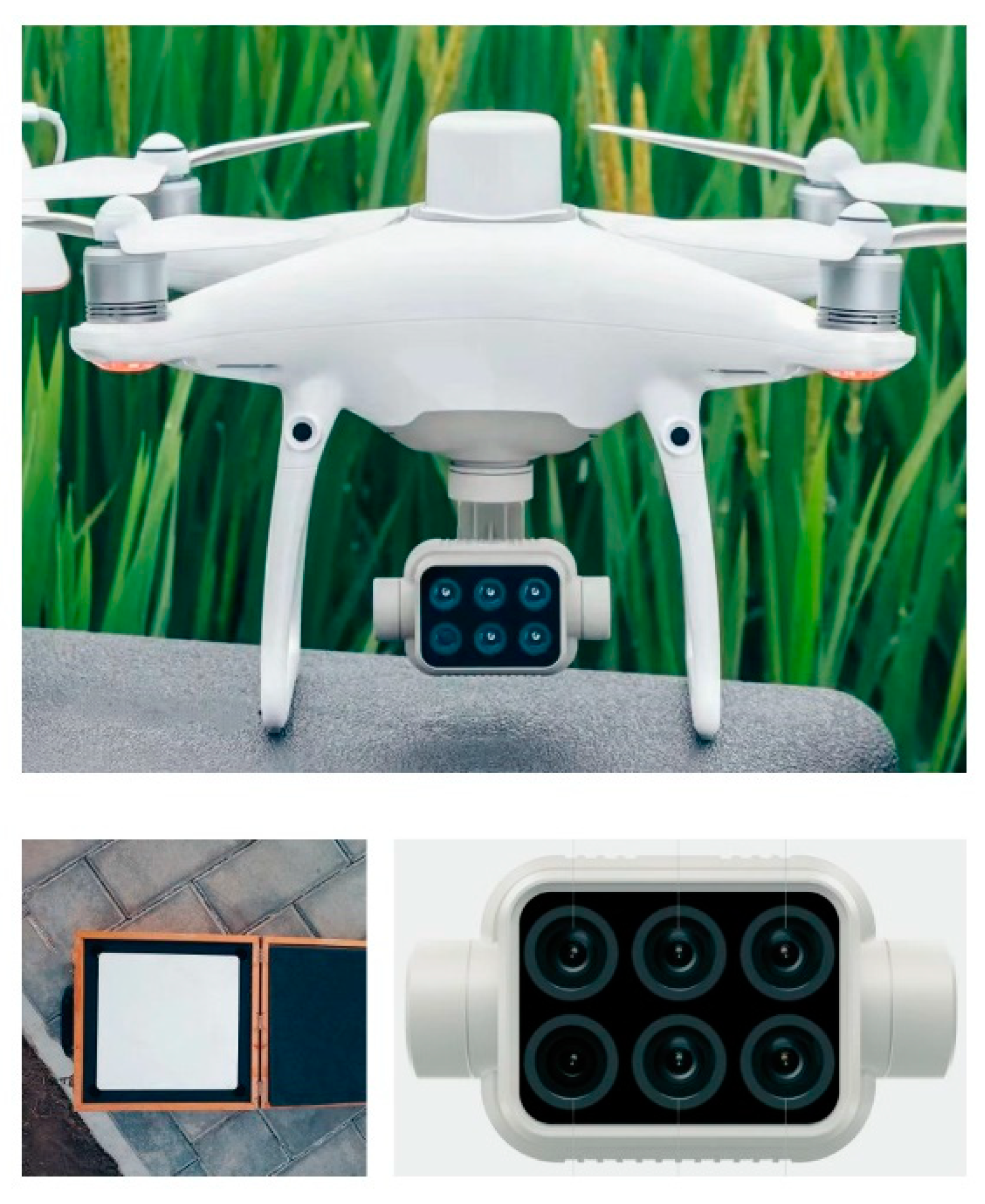
2.3.1. Acquisition and Pre-Processing

The flight platform uses a DJI P4 MULTISPECTRAL (P4M) quadrotor UAV with a take-off weight of 1.487 kg, a maximum flight altitude of 6000 m and a maximum horizontal flight speed of 58 km/h, as shown in Figure 2. The P4M takes an image sensor system with one color sensor for visible imaging with a 22 megapixel and five monochrome sensors for multispectral imaging, each with an effective pixel count of 2.08 million. The waveband information of the multispectral camera is shown in

Table 1. Band parameters of the multispectral sensor for P4M.

Waveband	Central Wavelength (nm)	Spectral Bandwidth (nm)	Panel Reflectance
Blue	450 ± 16	20	0.97
Green	560 ± 16	20	0.97
Red	650 ± 16	10	0.96
RedEdge	730 ± 16	10	0.95
NIR	840 ± 26	40	0.91

. The UAV imagery data observations were carried out at the jointing (5 July), booting (30 July) and filling (27 August) stages, with good light and stable wind speed during the flights. A calibrated reflectance whiteboard was set up before each experiment to obtain accurate reflectance data, the flight speed was set at 6 m/s and the height was set at 50 m, with a heading overlap rate of 80% and a side overlap rate of 70%. After the acquisition of the UAV images, the images were pre-processed using DJI Terra and Envi 5.31 software, as shown in Figure 3. The images were georeferenced for geometric correction using 10 uniformly distributed ground control points. A pseudo-standard feature radiometric correction method was used to convert the DN values of the multispectral image to reflectance from reflectance measured by a ground-based whiteboard. The white reference plate was measured with an ASD spectrometer before the UAV flight to facilitate the radiometric correction of the subsequent images, the DN values of the white reference cloth in each band were counted in the multispectral images and radiometric correction of the multispectral images was performed using the following equation:

$$\begin{array}{c}{\mathrm{R}}_{\mathrm{Target}}=\frac{{\mathrm{DN}}_{\mathrm{Target}}}{{\mathrm{DN}}_{\mathrm{Reference}\mathrm{plate}}}{\mathrm{R}}_{\mathrm{Reference}\mathrm{plate}}\end{array}$$

(1)

where the R target is the reflectance of the target feature, the DN target is the mean value of the DN of the target feature, the DN reference plate is the mean value of the DN of the white reference plate and the R reference plate is the reflectance value of the reference plate.

2.3.2. Image Fusion

Image fusion is an image processing technique that resamples digital images with a high spatial resolution and multispectral images with a high spectral resolution, aiming to generate a fused image with both a high spatial resolution and a high spectral resolution [34], which can fully exploit the advantages of multiple types of sensors in UAV remote sensing platforms.

The Gram–Schmidt Pan Sharpening (GS) fusion method selected in this study improves the shortcomings of the Principal Component Analysis (PCA) method, in which the information is too concentrated. GS is not limited by the band, can maintain spatial texture information well, especially the spectral feature information, and is designed for the latest high-spatial-resolution images [35]. Using the GS fusion method in ENVI5.3 to fuse the pre-processed multispectral and digital images at the pixel level, the advantages of the high spatial resolution of digital images and the high spectral resolution of multispectral images can be fully exploited, as shown in Figure 4.

2.3.3. Removal of Background Noise

Due to the high spatial resolution of UAV remote sensing imagery, the background noise such as soil, water and shadows of rice in the field will also be highlighted [36]. In this study, two transformations of HSV color space are used for the processed UAV digital images, as in Xu et al. [37] for corn, in which the first transformation can distinguish the rice canopy and water noise, and the second transformation can automatically classify the shadows on the leaves as leaves, thus separating the shadow noise faster and more accurately, as shown in Figure 5. The whole transformation process is based on the “RGB to HSV Color Transform” module, which is carried out in Envi5.31 software. It was then combined with a Random Forest classification algorithm (classes are rice, soil, water and shade; random_state = none; max_features = “auto”; min_samples_leaf = 2; accuracy is 90%) to remove the background noise and obtain an image of only the rice canopy, as shown in Figure 6. The whole classification process is based on the “Classification Workflow” module, which is available in Envi5.31.

2.4. Determining Input Variables for Modeling

2.4.1. Candidate Feature Variables

This study initially selected 19 vegetation indices (VIs) as candidate feature variables for estimating the LNC in the rice canopy based on the previous literature, as shown in

Table 2. Vegetation Indices used in this study.

Vegetation Index	Name	Formula	Ref
DVI	Difference Vegetation Index	Rnir − Rr	[38]
NDVI	Normalized Difference Vegetation Index	(Rnir − Rr)/(Rnir + Rr)	[39]
RDVI	Renormalized Difference Vegetation Index	(Rnir − Rr)/($\sqrt{R_{nir}/R_r}$)	[40]
GNDVI	Green Normalized Difference Vegetation Index	(Rnir − Rg)/(Rnir + Rg)	[41]
RVI	Ratio Vegetation Index	Rnir/Rr	[42]
GRVI	Green-Red Vegetation Index	(Rg − Rr)/(Rg + Rr)	[43]
WDRVI	Wide Dynamic Range Vegetation Index	(0.12Rnir − Rr)/(0.12Rnir + Rr)	[44]
NLI	Nonlinear Vegetation Index	(Rnir2 − Rr)/(Rnir2 + Rr)	[45]
MNLI	Modified Nonlinear Vegetation Index	(1.5Rnir2 − 1.5Rg)/(Rnir2 + Rr + 0.5)	[46]
SAVI	Soil-Adjusted Vegetation Index	(Rnir − Rr)/1.5(Rnir + Rr + 0.5)	[47]
OSAVI	Optimized Soil-Adjusted Vegetation Index	(Rnir − Rr)/(Rnir + Rr + 0.16)	[48]
TCARI	Transformed Chlorophyll Absorption Ratio Index	3 [(Rre − Rr) − 0.2(Rre − Rg)×(Rre/Rr)]	[49]
MCARI	Modified Chlorophyll Absorption Ratio Index	[(Rre − Rr) − 0.2(Rre − Rg)]×(Rre/Rr)	[50]
GCI	Green Chlorophyll Index	(Rnir/Rg) − 1	[51]
RECI	Red Edge Chlorophyll Index	(Rnir/Rre) − 1	[52]
EVI2	Two-band Enhanced Vegetation Index	2.5(Rnir − Rr)/(Rnir + 2.4Rr + 1)	[53]
NDREI	Normalized Difference Red Edge Index	(Rre − Rg)/(Rre + Rg)	[54]
MSRI	Modified Simple Ratio Index	(Rnir/Rr − 1)/($\sqrt{R_{nir}/R_r}+1$)	[55]
TVI	Triangular Vegetation Index	0.5(120(Rnir − Rre) − 200(Rr − Rre))	[49]

, which included typical nitrogen-related indices (NDVI, RDVI, GNDVI, NLI, MNLI, NDREI, MSRI, TVI), soil-regulated indices (DVI, SAVI, OSAVI, EVI2, RVI, GRVI, WDRVI) and additional chlorophyll-related indices (TCARI, MCARI, GCI, RECI). These chlorophyll indices were included as total leaf nitrogen indices and are often predominantly based on weak absorption features in the short-wave infrared, which are susceptible to the spectral features of moisture absorption, while for fresh crops that grow naturally, they usually contain more moisture, which is easy to cover up [4]. In addition, short-wave infrared bands are outside the spectral range of most multispectral UAV sensors. As much foliar nitrogen occurs in the form of chlorophyll, for fresh crops, chlorophyll-related indices are often used for nitrogen analysis.

Based on the radiation-corrected UAV images, a representative area with uniform growth is selected and combined with the GPS coordinates of the ground measured points, 24 plots are selected at each growth stage and the area of each plot is set to 900 pixels of 30 × 30. The size of the plot is expressed as the canopy area of a single rice plant on the UAV images. The reflectance of the five bands BLUE, GREEN, RED, REG and NIR was extracted from the 900 pixel points, and the average value was taken to construct the spectral feature variables in order to consider the structural variations greatly.

2.4.2. Feature Variable Selection

Since the feature variables often show correlation and collinearity, thus causing data redundancy and increasing the computational burden, this study optimized the initially selected feature variables to identify the optimal vegetation index for the estimation of the LNC in the rice canopy. In contrast to the traditional Pearson correlation analysis, this study selected:

• Successive Projections Algorithm (SPA)

SPA is a method of selecting the forward feature variable which uses the projection analysis of vectors to calculate by cycling through the projection of each wavelength on the other wavelengths in a loop, determine the wavelength with the largest projection value as the candidate wavelength and select the final feature wavelength based on the correction model [56]. The brief steps are as follows:

The initial iteration vector is $x_{k\left(0\right)}$, the number of variables to be extracted is N, the spectral matrix is denoted as column J, one of the optional selected spectral matrixes is column j and the jth column of the modeling set is assigned to $x_j$, denoted as $x_{k\left(0\right)}$.

The set of unselected column vectors is denoted as s,

$$\begin{array}{c}s=\left\{j,1\le j\le J,j\notin \left\{k\left(0\right),\cdots ,k\left(n-1\right)\right\}\right\}\end{array}$$

(2)

Calculate the projection of $x_j$ to the remaining column vectors separately and record it as $P_{xj}$,

$$\begin{array}{c}{P}_{xj}=x_j-\left(x_j^T{x}_{k\left(n-1\right)}\right)x_{k\left(n-1\right)}{\left(x_{k\left(n-1\right)}^T{x}_{k\left(n-1\right)}\right)}^{-1},j\in s\end{array}$$

(3)

The spectral wavelength for extracting the maximum projection vector is denoted as $k\left(n\right)$,

$$\begin{array}{c}k\left(n\right)=arg\left(max\left(\left|P_{xj}\right|\right),j\in s\right)\end{array}$$

(4)

Let $x_j$ = $P_x$, $j\in s$ and n = n + 1, if n < N, calculate circularly according to Formula (3).

The final extracted variable is $\left\{x_{k\left(n\right)}=0,\cdots N-1\right\}$. The k(0) and N corresponding to the smallest root mean squared error of interaction verification (RMSECV) in each loop is the optimal value [57].

2.

Competitive Adaptative Reweighted Sampling (CARS)

CARS is based on the Darwinian evolutionary principle of “survival of the fittest” and is a method for selecting feature variables by combining Monte Carlo sampling with the PLSR model regression coefficients. It uses adaptive weighted sampling to select the wavelengths with the largest absolute values of the regression coefficients in the PLS model and uses cross-validation to select the subset with the smallest RMSECV, thus finding the optimal variable combination [58]. The brief steps are as follows:

The Monte Carlo sampling method was used to build the PLS model, with the number of samples recorded as N, the absolute value of the regression coefficient of the ith variable recorded as $\left|b_i\right|$, the absolute value weight of the regression coefficient of the ith variable recorded as $w_i$ and the number of variables remaining in each sample recorded as m,

$$\begin{array}{c}{w}_i=\frac{\left|b_i\right|}{{{\displaystyle \sum }}_{i=1}^m\left|b_i\right|}\end{array}$$

(5)

The exponential decay function (EDF) is used to remove the value with the smaller absolute of the regression coefficient, and at the ith sampling, the ratio of the retained wavelength points obtained according to the EDF is denoted as $R_i$,

$$\begin{array}{c}{R}_i=\mu e^{-ki}\end{array}$$

(6)

In Formula (6), when the Nth sampling is completed, the ratio of the remaining wavelength points is 2/n, and n is the number of original wavelength points; then, the calculation formulas of μ and k are:

$$\begin{array}{c}\mu ={\left(\frac{n}{2}\right)}^{\frac{1}{N-1}}\end{array}$$

(7)

$$\begin{array}{c}k=\frac{\ln \left(\frac{n}{2}\right)}{N-1}\end{array}$$

(8)

At each sampling, the wavelength variable with the number of $R_i\times n$ is selected from the number of variables in the last time through adaptive weighted sampling, and the RMSECV is calculated by modeling. After N sampling, the wavelength variable corresponding to the minimum value of RMSECV is selected as the feature variable [59].

2.5. Modeling Methods

Based on the Jupyter Notebook IDE with Python, we used the sklearn, numpy, pandas, matplotlib and seaborn libraries, version 1.20.1, and two algorithms, Lasso Regression and Ridge Regression, were used to construct a remote sensing model for monitoring the rice LNC before and after GS fusion; the corresponding results were analyzed and compared. Among the common algorithms used for crop LNC modeling, we selected Random Forest (RF), an algorithm that integrates multiple decision trees through the idea of integration learning, for visual comparison.

2.5.1. LASSO Regression

The LASSO (Least Absolute Shrinkage and Selection Operator) algorithm, first proposed by (Tibshirani, R., 1993), has the property of compressing certain regression coefficients with small absolute values to zero by adding penalty terms so that some feature variables can be ignored and achieve simultaneous variable selection, which is called “L1 regularization” [60]. The LASSOCV model used in this study has a generalized cross-validation that can adaptively adjust the hyperparameter alpha to obtain the optimal model. The core formulas are as follows:

The dependent variable is $y={\left(y_1,\cdots ,y_n\right)}^T$, the independent variable is $X={\left(X_{1j},\cdots ,X_{nj}\right)}^T$, $j=1,\cdots p$, $\beta ={\left({\beta }_1,\cdots ,{\beta }_n\right)}^T$ is the vector coefficient and the basic linear model is:

$$\begin{array}{c}y=\beta X+\epsilon \end{array}$$

(9)

The variable selection and parameter estimation for LASSO are denoted as $\widehat{\beta }\left(LASSO\right)$, where λ is the regularization parameter,

$$\begin{array}{c}\widehat{\beta }\left(LASSO\right)=argmin{\displaystyle {\displaystyle \sum }_{i=1}^n}{\left(y_i-{\displaystyle {\displaystyle \sum }_{j=1}^p}{\beta }_j{X}_{ij}\right)}^2+\lambda {\displaystyle {\displaystyle \sum }_{j=1}^p}\left|{\beta }_j\right|\end{array}$$

(10)

2.5.2. RIDGE Regression

The RIDGE algorithm is a regression method of biased estimation for ill-posed problems, with the property of minimizing the regression coefficients in the model as much as possible and reducing the influence of each feature variable on the prediction results, thus preventing overfitting, which is called “L2 regularization” [61]. The RIDGECV model used in this study has generalized cross-validation and can be adaptively adjusted for the hyperparameter alpha to obtain the optimal model. The core formulas are as follows:

The dependent variable is $y={\left(y_1,\cdots ,y_n\right)}^T$, the independent variable is $X={\left(X_{1j},\cdots ,X_{nj}\right)}^T$, $j=1,\cdots p$, $\beta ={\left({\beta }_1,\cdots ,{\beta }_n\right)}^T$ is the vector coefficient and the basic linear model is:

$$\begin{array}{c}y=\beta X+\epsilon \end{array}$$

(11)

The variable selection and parameter estimation for RIDGE are denoted as $\widehat{\beta }\left(RIDGE\right)$, where λ is the regularization parameter,

$$\begin{array}{c}\widehat{\beta }\left(RIDGE\right)=argmin{\displaystyle {\displaystyle \sum }_{i=1}^n}{\left(y_i-{\displaystyle {\displaystyle \sum }_{j=1}^p}{\beta }_j{X}_{ij}\right)}^2+\lambda {\displaystyle {\displaystyle \sum }_{j=1}^p}{\beta }_j^2\end{array}$$

(12)

2.6. Evaluation Indicators

Compared with the traditional hold-out method, this study used the K-Fold Cross Validation method based on the K-Fold module from the sklearn library on Jupyter Notebook IDE with Python. This method can divide the overall data into K parts on average, each time taking one subset of data as the test set and the remaining K − 1 subsets as the training set, repeating K times, and the results are weighted and averaged to reduce the inaccuracy of the training results and improve the utilization of the data [62].

To evaluate the precision and accuracy of the model, three indicators are selected: Coefficient of Determination (R²), Root Mean Square Error (RMSE) and Normalized Root Mean Square Error (NRMSE). The larger R² is, the better the model fits, and the smaller the RMSE and NRMSE are, the more accurate the model is. The formulas for their calculation are shown below:

$$\begin{array}{c}{R}^2=1-\frac{{{\displaystyle \sum }}_{i=1}^n{\left(x_i-y_i\right)}^2}{{{\displaystyle \sum }}_{i=1}^n{\left(x_i-\overline{x}\right)}^2}\end{array}$$

(13)

$$\begin{array}{c}RMSE=\sqrt{\frac{{{\displaystyle \sum }}_{i=1}^n{\left(y_i-x_i\right)}^2}{n}}\end{array}$$

(14)

$$\begin{array}{c}NRMSE=\frac{RMSE}{\overline{X}}\end{array}$$

(15)

In the formula, $x_i$ represents the measured value of the rice canopy LNC, $\overline{x}$ represents the average value of the measured value, $y_i$ represents the predicted value of the rice canopy LNC and n represents the number of samples of the model.

3. Results and Analysis

3.1. Descriptive Statistics

The LNC (g 100 g⁻¹, %) of rice varied greatly under different growth stages and nitrogen application conditions, as shown in

Table 3. Descriptive statistics for the rice leaf nitrogen content (LNC) at different growth stages.

Growth Stage	Samples	Min	Max	Mean	Standard Deviation	Coefficient of Variation (%)
Jointing	24	3.95	4.65	4.34	0.21	4.84
Booting	24	3.34	3.89	3.67	0.16	4.36
Filling	24	2.89	3.52	3.13	0.17	5.43

. The overall range of LNC values for rice at the jointing stage was the largest, at 3.95–4.65%, and its overall range of LNC values gradually decreased as the rice developed. The descriptive statistics of LNC in the rice canopy showed that the coefficient of variation (CV) ranged between 4.36% and 5.43%, expressing little variation in LNC between the application treatments, and the data can be applied normally, which also made it possible to use UAV remote sensing data for the LNC estimation of rice canopy.

Figure 7 shows the Pearson correlation coefficients between the vegetation indices (VIs) and the LNC based on multispectral imagery at different growth stages. It can be observed that the overall correlation coefficient is higher at the jointing stage than it is at the booting and filling stages. Compared with the other indices, OSAVI, MCARI and TVI showed a better correlation with the LNC in the rice canopy at all growth stages.

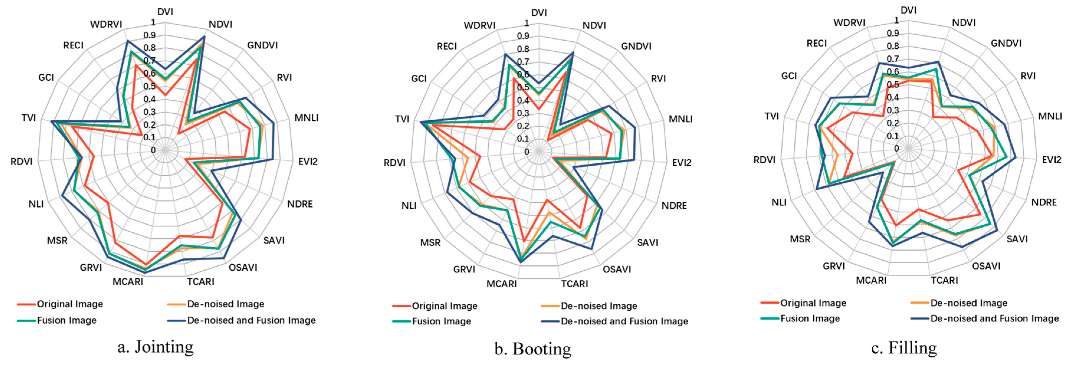
3.2. Correlation Analysis of Feature Variables

For three growth stages (the jointing, booting and filling stages), UAV multispectral images were extracted as raw images. The GS fusion method was applied to original images to obtain the fused images, and then the HSV transformation was applied to the original images and the fused images, respectively, to remove the background noise and obtain the denoised images and the fused-denoised images.

Pearson correlation analysis was conducted between the spectral feature variables constructed from the four images with the measured rice LNC data; the results for each growth stage are shown in Figure 8. The correlation between the feature variables and the LNC of rice was better in the denoised image and fusion image than it was in the original image for all three growth stages, indicating that the feature variables extracted from the processed images were more accurate and that the denoised and fusion image correlated best. In terms of the overall growth period of rice, the correlation between the feature variables and LNC was best at the jointing stage.

3.3. Extraction of Optimal Feature Variables

The SPA and the CARS method were compared to further extract the feature variables. The SPA algorithm was first used to optimize the feature variables, first setting the number of feature variables to 2–19 and then extracting the final number of variables, which was determined by the minimum RMSE. As can be seen in Figure 9, as the number of feature variables increased, the RMSE showed a decreasing trend, with the smallest value being 0.19623 when the number of input variables was three, followed by an increasing RMSE as the number of variables increased further, reaching a plateau at 15. This is because too many variables will increase the mutual collinearity and redundancy, leading to a decrease in the model accuracy. Taking the original multispectral images at the jointing stage as an example, three feature variables were selected, with variable sequences of 7, 10 and 12, and the corresponding vegetation indices are: SAVI, TCARI and GRVI.

The CARS algorithm was used for feature selection, and the number of Monte Carlo MC samples was set to 50. The minimum RMSE was used to determine the number of variables to be extracted. As can be seen in Figure 10a, the RMSE of the model varies from small to large as the number of MC samples increases from a range of 0 to 50 until it reaches a minimum of 0.127 at a sampling frequency of 25. As can be seen in Figure 10b, due to the exponential decay function (EDA), the feature variables decrease rapidly in the early stages of sampling and slow down gradually as the number of samples increases, indicating that the algorithm has two processes: “rough selection” and “fine selection”. When the number of samples was 25, the corresponding number of input variables was five. Taking the original multispectral images at the jointing stage as an example, five feature variables were selected, corresponding to the vegetation indices SAVI, OSAVI, MSR, RDVI and WDRVI.

3.4. Modeling of LNC Using Machine Learning Algorithms

3.4.1. Results of GS Fusion

In this section, the GS fusion method was used to obtain the corresponding fusion image, and the two regularization algorithms, LASSO and RIDGE, were compared to commonly used RF algorithms to analyze the original data. Spectral images and fusion images were used to construct a model for monitoring the canopy LNC in rice, and the results are shown in

Table 4. Predictive performance of Rice LNC using the RF, LASSO and RIDGE algorithms for both original and fusion images.

Growth Stage	Condition	Number of Variables	Selected Feature Variables	Method	R2	RMSE (%)	NRMSE (%)
Jointing	Original Image	5	MCARI, GRVI, OSAVI, NDVI, TVI	RF	0.43	14.87	3.43
		19 (3)	MCARI, GRVI, TCARI	LASSO	0.57	13.41	3.09
		5	MCARI, GRVI, OSAVI, NDVI, TVI	RIDGE	0.52	14.43	3.32
	Fusion Image	5	MCARI, WDRVI, GRVI, OSAVI, MNLI	RF	0.50	13.56	3.13
		19 (3)	MCARI, GRVI, SAVI	LASSO	0.66	11.96	2.76
		5	MCARI, WDRVI, GRVI, OSAVI, MNLI	RIDGE	0.60	13.48	3.11
Booting	Original Image	5	OSAVI, NDVI, TVI, MCARI, WDRVI	RF	0.40	11.72	3.19
		19 (5)	OSAVI, TVI, MCARI, WDRVI, NLI	LASSO	0.51	10.86	2.96
		5	OSAVI, NDVI, TVI, MCARI, WDRVI	RIDGE	0.48	11.36	3.09
	Fusion Image	5	OSAVI, TVI, MCARI, NDVI, NLI	RF	0.48	11.53	3.14
		19 (5)	OSAVI, TVI, NDVI, MCARI, WDRVI	LASSO	0.57	11.16	3.04
		5	OSAVI, TVI, MCARI, NDVI, NLI	RIDGE	0.55	11.41	3.11
Filling	Original Image	5	SAVI, EVI2, OSAVI, TVI, MCARI	RF	0.36	13.35	4.26
		19 (4)	SAVI, WDRVI, TVI, MCARI	LASSO	0.47	12.66	4.05
		5	SAVI, EVI2, OSAVI, TVI, MCARI	RIDGE	0.44	13.09	4.18
	Fusion Image	5	SAVI, OSAVI, TVI, MNLI, NDVI	RF	0.45	11.91	3.81
		19 (4)	SAVI, OSAVI, MNLI, NLI	LASSO	0.53	11.13	3.56
		5	SAVI, OSAVI, TVI, MNLI, NDVI	RIDGE	0.51	11.68	3.73

Note: 19 (3) indicates that the model has 19 input variables and that the LASSO algorithm has selected 3 variables.

. The RIDGE and RF regression algorithm was based on the Pearson correlation analysis above, and the five feature variables with the best correlation in each case were selected, while the LASSO regression algorithm input the full feature variable (19 feature variables) in the modeling due to its dimensionality reduction feature, and the feature variable selection was performed by the algorithm itself.

As can be seen in Table 4, the accuracy of the prediction model based on fusion images was improved at all growth stages, and the R² of the fusion model could be improved by 7%, on average, compared to the original multispectral images. Under the same conditions, the regularization algorithms were better than the RF algorithm, with the LASSO regression being the best. The model predictions for each growth stage are shown in Figure 11.

3.4.2. Results of Removing Background Noise

The monitoring model of rice LNC is constructed by combining the RF, Lasso and Ridge algorithms for the original multispectral images, the fused images and the corresponding images after removing the background noise for the UAV image data at the rice jointing, booting and filling stages. The results are shown in

Table 5. Predictive performance of LNC using the RF, LASSO and RIDGE algorithms for both the original and fusion images and the corresponding denoised image.

Growth Stage	Condition	Number of Variables	Selected Feature Variables	Method	R2	RMSE (%)	NRMSE (%)
Jointing	Original Image	5	MCARI, GRVI, OSAVI, NDVI, TVI	RF	0.43	14.87	3.43
		19 (3)	MCARI, GRVI, TCARI	LASSO	0.57	13.41	3.09
		5	MCARI, GRVI, OSAVI, NDVI, TVI	RIDGE	0.52	14.43	3.32
	Denoised Original Image	5	MCARI, GRVI, WDRVI, SAVI, NDVI	RF	0.48	13.86	3.19
		19 (5)	MCARI, SAVI, NDVI, WDRVI, TVI	LASSO	0.63	12.72	2.93
		5	MCARI, GRVI, WDRVI, SAVI, NDVI	RIDGE	0.58	13.57	3.13
	Fusion Image	5	MCARI, WDRVI, GRVI, OSAVI, MNLI	RF	0.50	13.56	3.13
		19 (3)	MCARI, GRVI, SAVI	LASSO	0.66	11.96	2.76
		5	MCARI, WDRVI, GRVI, OSAVI, MNLI	RIDGE	0.60	13.48	3.11
	Denoised Fusion Image	5	MCARI, WDRVI, GRVI, OSAVI, NLI	RF	0.57	12.43	2.87
		19 (6)	MCARI, GRVI, SAVI, NLI, TVI, RVI	LASSO	0.69	11.36	2.62
		5	MCARI, WDRVI, GRVI, OSAVI, NLI	RIDGE	0.66	12.09	2.79
Booting	Original Image	5	OSAVI, NDVI, TVI, MCARI, WDRVI	RF	0.40	11.72	3.19
		19 (5)	OSAVI, TVI, MCARI, WDRVI, NLI	LASSO	0.51	10.86	2.96
		5	OSAVI, NDVI, TVI, MCARI, WDRVI	RIDGE	0.48	11.36	3.09
	Denoised Original Image	5	OSAVI, NDVI, WDRVI, NLI, MNLI	RF	0.45	11.59	3.16
		19 (3)	OSAVI, NDVI, WDRVI	LASSO	0.55	10.34	2.82
		5	OSAVI, NDVI, WDRVI, NLI, MNLI	RIDGE	0.53	11.24	3.06
	Fusion Image	5	OSAVI, TVI, MCARI, NDVI, NLI	RF	0.48	11.53	3.14
		19 (5)	OSAVI, TVI, NDVI, MCARI, WDRVI	LASSO	0.57	11.16	3.04
		5	OSAVI, TVI, MCARI, NDVI, NLI	RIDGE	0.55	11.41	3.11
	Denoised Fusion Image	5	TVI, WDRVI, OSAVI, MCARI, NLI	RF	0.52	11.17	3.04
		19 (4)	TVI, OSAVI, MCARI, NLI	LASSO	0.62	9.79	2.67
		5	TVI, WDRVI, OSAVI, MCARI, NLI	RIDGE	0.59	10.83	2.95
Filling	Original Image	5	SAVI, EVI2, OSAVI, TVI, MCARI	RF	0.36	13.35	4.26
		19 (4)	SAVI, WDRVI, TVI, MCARI	LASSO	0.47	12.66	4.05
		5	SAVI, EVI2, OSAVI, TVI, MCARI	RIDGE	0.44	13.09	4.18
	Denoised Original Image	5	SAVI, TVI, OSAVI, MCARI, NLI	RF	0.41	14.11	4.51
		19 (3)	SAVI, TVI, OSAVI	LASSO	0.52	11.79	3.77
		5	SAVI, TVI, OSAVI, MCARI, NLI	RIDGE	0.49	13.83	4.42
	Fusion Image	5	SAVI, OSAVI, TVI, MNLI, NDVI	RF	0.45	11.91	3.81
		19 (4)	SAVI, OSAVI, MNLI, NLI	LASSO	0.53	11.13	3.56
		5	SAVI, OSAVI, TVI, MNLI, NDVI	RIDGE	0.51	11.68	3.73
	Denoised Fusion Image	5	SAVI, EVI2, GCI, OSAVI, MCARI	RF	0.49	10.98	3.51
		19 (4)	SAVI, OSAVI, MCARI, EVI2	LASSO	0.58	9.68	3.09
		5	SAVI, EVI2, GCI, OSAVI, MCARI	RIDGE	0.54	10.77	3.44

Note: 19 (3) indicates that the model has 19 input variables and that the LASSO algorithm has selected 3 variables.

.

It can be seen in Table 5 that, at all growth stages, the accuracy of the prediction model based on denoised images was improved. Among them, the R² of the original multispectral model can be increased by 5%, on average, compared to the denoised images, and the R² of the fusion image can be increased by 4%, on average, after being denoised. Under the same conditions, the regularization algorithms were better than the RF algorithm, with the effect of LASSO being a little better than that of RIDGE. The model predictions for each growth stage are shown in Figure 12.

3.4.3. Results of the Optimal Feature Variable Prediction

For the denoised multispectral images and fused images at the rice jointing, booting and filling stages, we also considered using RF, LASSO, RIDGE, RIDGE-SPA (RR-SPA) and RIDGE-CARS (RR-CARS) to construct a model for monitoring the canopy LNC in rice. The results are shown in

Table 6. Predictive performance of Rice LNC using the RF, LASSO, RIDGE, RR-SPA and RR-CARS algorithms for denoised original MS and fusion images.

Growth Stage	Condition	Number of Variables	Selected Feature Variables	Method	R2	RMSE (%)	NRMSE (%)
Jointing	Denoised Original Image	5	MCARI, GRVI, WDRVI, SAVI, NDVI	RF	0.48	13.86	3.19
		19 (5)	MCARI, SAVI, NDVI, WDRVI, TVI	LASSO	0.63	12.72	2.93
		5	MCARI, GRVI, WDRVI, SAVI, NDVI	RIDGE	0.58	13.57	3.13
		3	MCARI, SAVI, WDRVI	RR-SPA	0.68	12.05	2.78
		5	MCARI, GRVI, SAVI, WDRVI, NLI	RR-CARS	0.64	12.22	2.82
	Denoised Fusion Image	5	MCARI, WDRVI, GRVI, OSAVI, NLI	RF	0.57	12.43	2.87
		19 (6)	MCARI, GRVI, SAVI, NLI, TVI, RVI	LASSO	0.69	11.36	2.62
		5	MCARI, WDRVI, GRVI, OSAVI, NLI	RIDGE	0.66	12.09	2.79
		3	MCARI, SAVI, OSAVI	RR-SPA	0.76	10.33	2.38
		5	MCARI, SAVI, GRVI, NLI, TVI	RR-CARS	0.70	11.26	2.59
Booting	Denoised Original Image	5	OSAVI, NDVI, WDRVI, NLI, MNLI	RF	0.45	11.59	3.16
		19 (3)	OSAVI, NDVI, WDRVI	LASSO	0.55	10.34	2.82
		5	OSAVI, NDVI, WDRVI, NLI, MNLI	RIDGE	0.53	11.24	3.06
		3	OSAVI, WDRVI, MCARI	RR-SPA	0.62	9.66	2.63
		7	NDVI, NLI, TVI, RVI, MNLI, OSAVI, EVI2	RR-CARS	0.54	10.91	2.98
	Denoised Fusion Image	5	TVI, WDRVI, OSAVI, MCARI, NLI	RF	0.52	11.17	3.04
		19 (4)	TVI, OSAVI, MCARI, NLI	LASSO	0.62	9.79	2.67
		5	TVI, WDRVI, OSAVI, MCARI, NLI	RIDGE	0.59	10.83	2.95
		3	TVI, WDRVI, MCARI	RR-SPA	0.71	8.83	2.41
		7	NDVI, NLI, TVI, RVI, MNLI, OSAVI, GCI	RR-CARS	0.63	9.74	2.66
Filling	Denoised Original Image	5	SAVI, TVI, OSAVI, MCARI, NLI	RF	0.41	14.11	4.51
		19 (3)	SAVI, TVI, OSAVI	LASSO	0.52	11.79	3.77
		5	SAVI, TVI, OSAVI, MCARI, NLI	RIDGE	0.49	13.83	4.42
		3	SAVI, OSAVI, MCARI	RR-SPA	0.58	11.36	3.63
		6	SAVI, WDRVI, TVI, NLI, NDVI, OSAVI	RR-CARS	0.53	12.01	3.84
	Denoised Fusion Image	5	SAVI, EVI2, GCI, OSAVI, MCARI	RF	0.49	10.98	3.51
		19 (4)	SAVI, OSAVI, MCARI, EVI2	LASSO	0.58	9.68	3.09
		5	SAVI, EVI2, GCI, OSAVI, MCARI	RIDGE	0.54	10.77	3.44
		3	MCARI, SAVI, OSAVI	RR-SPA	0.67	8.76	2.80
		6	EVI2, NLI, TVI, MCARI, OSAVI, RVI	RR-CARS	0.61	9.30	2.97

Note: 19 (3) indicates that the model has 19 input variables and that the LASSO algorithm has selected 3 variables.

. The RR-SPA algorithm is based on the SPA for optimal feature variable selection, and the RR-CARS algorithm was based on the CARS.

It can be seen in Table 6 that the R² of the models optimized by the SPA and CARS algorithms has been improved in all growth stages. Among them, for the denoised original multispectral image, the R² of the RIDGE model based on SPA optimization is increased by 9%, on average, and the R² of the RIDGE model based on CARS optimization is increased by 4%, on average, compared to the RIDGE model alone; for the denoised fusion image, the R² of the SPA-optimized RIDGE model is increased by an average of 12%, and the R² of the CARS-optimized RIDGE model is improved by an average of 5% compared to the original RIDGE model.

Overall, when establishing the remote sensing model for monitoring canopy LNC in rice, the regularization algorithms are better than the traditional RF algorithm, and the effect of RR-SPA is the best, followed by RR-CARS and LASSO; the worst is the RIDGE algorithm model. The model predictions for each growth period are shown in Figure 13.

3.5. Construction of the Spatial Distribution Map of LNC

By comparing the LNC estimation models of different treatments and modeling methods, it was found that the model using RIDGE regression combined with the SPA algorithm achieved the best results. Therefore, the optimal and specific model for each growth stage was applied to construct a spatial distribution map of LNC in the rice fields, and the results are shown in Figure 14.

It can be seen that the predicted value of LNC gradually decreased from the jointing to the filling stage, which is in line with the measured results. The growth condition of rice varied between the plots due to the different N fertilizer applications. The predicted values of LNC in plots N2–N5 were less different, probably due to the small differences in the fertilizer application between the plots, but the overall prediction accuracy was good. The rice growth in plots N1 and N6 was average, probably due to the higher N fertilizer application in plot N1 and the low N fertilizer application in plot N6. The highest predicted values of rice LNC ranged from 4.01 to 4.61% at the jointing stage and from 3.42 to 3.87% at the booting stage, and the lowest predicted values of LNC ranged from 2.92 to 3.39% at the filling stage, which may be related to the growth and development of the spike and the background noise generated; the overall situation was consistent with the experimental results in the field.

4. Discussion

In this paper, the UAV image data are processed based on image fusion methods and background noise removal, and monitoring models of canopy LNC in rice are evaluated through comparing methods of optimizing feature variables such as SPA and CARS, combined with the RF, LASSO and RIDGE regression algorithms.

4.1. Nitrogen Estimation for Different Image Treatments

UAV remote sensing technology is widely used because it is low-cost, fast and convenient, can collect data in real time and has an excellent spatial resolution of the imaging. However, most previous studies based on UAV remote sensing have used a single RGB or a multispectral sensor, failing to fully exploit the advantages of UAV remote sensing platforms and multiple sensors, resulting in insufficient acquired information and the poor prediction accuracy of the models [4,5,8]. In contrast, there are also studies based on satellite remote sensing that have used GS fusion methods and achieved good results [34,35]. In this study, the GS method was used to fuse images from two sensors mounted on the UAV, RGB and multispectral cameras to obtain fused images with both a high spatial resolution and high spectral resolution (Figure 4), which indicates that it is feasible to fuse images with the GS method, which may have implications for other studies.

As UAV RGB imagery has a high spatial resolution, it contains more feature information. Similarly, more background noise such as soil, shadows, etc. is highlighted, so, in UAV remote sensing applications, it is important to first consider how to reduce the removal of noise from the background. In previous studies, the removal of soil background noise from dryland crops such as corn, wheat and potatoes was more often achieved by converting RGB images to HSV color space [63,64,65], but the major difference between rice and them is the growing environment. Rice seedlings require transplanting, regular irrigation and other water treatments, which means that there are effects not only from soil and shadow but also from water on the image. In this study, the HSV color space transform was used to remove the influence of soil and shadows from the UAV RGB images. In particular, this study used two HSV color space transforms to identify water and shadows well (Figure 5) and then combined them with supervised classification algorithms such as random forest to separate out pure vegetation well (Figure 6), which may have implications for other related studies.

The correlation between the vegetation index and the LNC of rice was significantly improved for the fused and background noise-removed images compared to that for the unprocessed original images (Figure 8). In the former case, this is probably due to the fact that the pixel-based fusion absorbs features from different sensors and contains rich data, resulting in more information being obtained. For the latter, this is mainly because the vegetation index is calculated by averaging the entire image pixels in the image, and the sample points with and without background noise removed occupy significantly different pixel points; after image processing, only the vegetation section will be used for the vegetation index calculation, which also enhances the accuracy of the prediction model. This variation is also evidenced by the model effects for each case in Table 5. The main difference between these studies and the current study is that the crops are grown in different environments, meaning they have different background noises. The imagery processing used in this study for rice could be a reference.

4.2. Nitrogen Estimation for Different Modeling Approaches

Pearson correlation analysis is widely used to select variables in monitoring models because of its convenience and speed. However, the results of its selection can only show that the variables are correlated with the predictive target and cannot eliminate redundancy between variables [16,17]. Conversely, there have also been many studies that have filtered out duplicate information between variables by using algorithms that can optimize the spectral feature variables [15,18,19], while for the SPA and CARS algorithms, they are more widely used in estimation models based on hyperspectral data and have achieved a good model accuracy [20,21], as hyperspectral data usually have hundreds of bands, and the possibility of redundant duplication is greater, but this does not mean that it is not necessary for multispectral data. In this study, the SPA and CARS algorithms were used to screen vegetation indices in a multispectral image-based LNC prediction model for rice, and the prediction accuracy of the established model was significantly improved compared to that of the traditional Pearson method, which proved that it is feasible to use algorithms such as SPA or CARS, which can effectively eliminate redundancy and crosstalk problems in spectral data and improve the accuracy of the model.

Remote sensing monitoring models are usually built using standard statistical models or machine learning-based regression algorithms. Statistical models place more emphasis on exploring the relationship between remote sensing information and crops through mathematical statistical methods and logical inference, and although many studies have shown that these models are very interpretable [25,26,27], they are not very accurate and are generally only applicable to smaller amounts of data and narrower data attributes. In contrast, although machine learning-based regression algorithms and statistical models are both branches of artificial intelligence, they rely more on data learning, focus more on model optimization and performance and can usually process large amounts of data quickly and achieve a high prediction accuracy.

In this study, on the basis of the traditional regression algorithm, two sibling algorithms based on regularization are also chosen: the LASSO algorithm and the RIDGE algorithm. Regularization here can reduce the complexity of the model by imposing penalty factors to lower the weight values of the parameters, where the LASSO algorithm has the advantage of dimensionality reduction when applied in isolation, while the RIDGE algorithm can effectively prevent overfitting. With the LASSO and RIDGE algorithms, we found that the accuracy of the model was improved when compared with the traditional RF algorithm (Table 4 and Table 5), which is consistent with the results of Ku et al. [29] and Piepho et al. [30]. When they were combined with the feature preference algorithm, the model was further improved (Table 6), which proves that they are effective. This may have implications for other related studies.

4.3. Future Research Prospects

In this study, processed UAV images and a machine learning algorithm combining the optimal feature variable algorithm were used to predict the LNC of rice, although some soil and shadows could not be completely removed due to the effect of the camera angle and the solar irradiation angle on the UAV. Additionally, the accuracy of the model was affected during the booting and filling stages, possibly due to the growth and development of the rice spike. However, the prediction accuracy of the model was still improved by image processing methods of image fusion and background noise removal. The results show that we can monitor the growth of rice in real time and quickly so that we can determine the N content of a site and decide whether to continue to fertilize it in order to make precise and quantitative fertilization decisions. For future research, in order to consider how to remove the rice spikes to further enhance the removal of background noise from the images, we need to analyze, in detail, the results of the adopted HSV transform with supervised classification for image segmentation, which may involve more semantic segmentation aspects of remote sensing images, which are often complex, and we consider data enhancement to obtain more images as datasets and use convolutional neural networks in deep learning to conduct deeper processing and research. For algorithms in the future, we should consider using deep learning algorithms to predict the nutritional status of rice, which is used in many vegetation-based classification problems but hardly ever for crop LNC prediction; it usually requires scaling up experiments and acquiring more data than just those based on vegetation index variables. In addition to this, the method used to determine the LNC may also have an impact on the results. The conventional Kjeldahl method of nitrogen determination was used in this study, and in the future, further research should be carried out by comparing it with other methods such as the indophenol blue colorimetric method. The field methodology used in this study is inappropriate; this led to a possible bias in our sampling, which was not well conducted in terms of randomness and repeatability. In future studies, we will consider using a random nitrogen treatment rather than a uniform growth area, which may improve the accuracy of the model.

5. Conclusions

This study estimates the rice canopy LNC based on UAV digital RGB and multispectral images. The UAV images are pre-processed by a GS fusion method and two transformations of HSV color space combined with RF classification algorithms. The aim is to explore the potential of methods for optimizing feature variables, such as SPA and CARS, combined with machine learning techniques, such as LASSO and RIDGE, in developing remote sensing models for monitoring the growth parameters in crops. We compared the accuracy of these models and found out that the fusion images obtained by the GS fusion method have both a high spatial resolution and a high spectral resolution, and the accuracy of modeling with fusion images is higher than that of the original multispectral images. Using two transformations of HSV color space combined with the RF classification algorithm can effectively separate rice, water, soil and shadows in rice fields, thus achieving the purpose of removing background noise. The accuracy of modeling with the denoised image is higher than that of the original multispectral image. The redundancy and collinearity between variables can be reduced through the use of methods for optimizing feature variables such as SPA and CARS. After combining it with the RIDGE algorithm, the accuracy of the model has been improved. Our results provide a reference for the estimation of canopy LNC in rice and the decision of accurate fertilization in rice fields.

References

1. Inoue, Y.; Sakaiya, E.; Zhu, Y.; Takahashi, W. Diagnostic mapping of canopy nitrogen content in rice based on hyperspectral measurements. Remote Sens. Environ. 2012, 126, 210–221. [Google Scholar] [CrossRef]
2. Qiu, Z.; Ma, F.; Li, Z.; Xu, X.; Ge, H.; Du, C. Estimation of nitrogen nutrition index in rice from UAV RGB images coupled with machine learning algorithms. Comput. Electron. Agric. 2021, 189, 106421. [Google Scholar] [CrossRef]
3. Wu, W.; Ma, B. Integrated nutrient management (INM) for sustaining crop productivity and reducing environmental impact: A review. Sci. Total Environ. 2015, 512, 415–427. [Google Scholar] [CrossRef] [PubMed]
4. Fu, Y.; Yang, G.; Li, Z.; Song, X.; Li, Z.; Xu, X.; Wang, P.; Zhao, C. Winter Wheat Nitrogen Status Estimation Using UAV-Based RGB Imagery and Gaussian Processes Regression. Remote Sens. 2020, 12, 3778. [Google Scholar] [CrossRef]
5. Shi, P.; Wang, Y.; Xu, J.; Zhao, Y.; Yang, B.; Yuan, Z.; Sun, Q. Rice nitrogen nutrition estimation with RGB images and machine learning methods. Comput. Electron. Agric. 2021, 180, 105860. [Google Scholar] [CrossRef]
6. Sun, J.; Ye, M.; Peng, S.; Li, Y. Nitrogen can improve the rapid response of photosynthesis to changing irradiance in rice (Oryza sativa L.) plants. Sci. Rep. 2016, 6, srep31305. [Google Scholar] [CrossRef] [PubMed]
7. Wang, L.; Chen, S.; Li, D.; Wang, C.; Jiang, H.; Zheng, Q.; Peng, Z. Estimation of Paddy Rice Nitrogen Content and Accumulation Both at Leaf and Plant Levels from UAV Hyperspectral Imagery. Remote Sens. 2021, 13, 2956. [Google Scholar] [CrossRef]
8. Ge, H.; Xiang, H.; Ma, F.; Li, Z.; Qiu, Z.; Tan, Z.; Du, C. Estimating Plant Nitrogen Concentration of Rice through Fusing Vegetation Indices and Color Moments Derived from UAV-RGB Images. Remote Sens. 2021, 13, 1620. [Google Scholar] [CrossRef]
9. Colorado, J.D.; Cera-Bornacelli, N.; Caldas, J.S.; Petro, E.; Rebolledo, M.C.; Cuellar, D.; Calderon, F.; Mondragon, I.F.; Jaramillo-Botero, A. Estimation of Nitrogen in Rice Crops from UAV-Captured Images. Remote Sens. 2020, 12, 3396. [Google Scholar] [CrossRef]
10. Zheng, H.; Cheng, T.; Li, D.; Zhou, X.; Yao, X.; Tian, Y.; Cao, W.; Zhu, Y. Evaluation of RGB, Color-Infrared and Multispectral Images Acquired from Unmanned Aerial Systems for the Estimation of Nitrogen Accumulation in Rice. Remote Sens. 2018, 10, 824. [Google Scholar] [CrossRef] [Green Version]
11. Loukatos, D.; Templalexis, C.; Lentzou, D.; Xanthopoulos, G.; Arvanitis, K.G. Enhancing a flexible robotic spraying platform for distant plant inspection via high-quality thermal imagery data. Comput. Electron. Agric. 2021, 190, 106462. [Google Scholar] [CrossRef]
12. Kerkech, M.; Hafiane, A.; Canals, R. Deep leaning approach with colorimetric spaces and vegetation indices for vine diseases detection in UAV images. Comput. Electron. Agric. 2018, 155, 237–243. [Google Scholar] [CrossRef]
13. Reza, M.N.; Na, I.; Baek, S.; Lee, I.; Lee, K. Lab Color Space based Rice Yield Prediction using Low Altitude UAV Field Image. In Proceedings of the Proceedings of the KSAM & UMRC 2017 Spring Conference, Gunwi-Gun, Republic of Korea, 7 April 2017. [Google Scholar]
14. Zhou, D.; Li, M.; Li, Y.; Qi, J.; Liu, K.; Cong, X.; Tian, X. Detection of ground straw coverage under conservation tillage based on deep learning. Comput. Electron. Agric. 2020, 172, 105369. [Google Scholar] [CrossRef]
15. Chen, Z.; Jia, K.; Xiao, C.; Wei, D.; Zhao, X.; Lan, J.; Wei, X.; Yao, Y.; Wang, B.; Sun, Y.; et al. Leaf Area Index Estimation Algorithm for GF-5 Hyperspectral Data Based on Different Feature Selection and Machine Learning Methods. Remote Sens. 2020, 12, 2110. [Google Scholar] [CrossRef]
16. Shicheng, Q.; Youwen, T.; Qinghu, W.; Shiyuan, S.; Ping, S. Nondestructive detection of decayed blueberry based on information fusion of hyperspectral imaging (HSI) and low-Field nuclear magnetic resonance (LF-NMR). Comput. Electron. Agric. 2021, 184, 106100. [Google Scholar] [CrossRef]
17. Ng, W.; Minasny, B.; Malone, B.P.; Sarathjith, M.C.; Das, B.S. Optimizing wavelength selection by using informative vectors for parsimonious infrared spectra modelling. Comput. Electron. Agric. 2019, 158, 201–210. [Google Scholar] [CrossRef]
18. Jia, M.; Li, W.; Wang, K.; Zhou, C.; Cheng, T.; Tian, Y.; Zhu, Y.; Cao, W.; Yao, X. A newly developed method to extract the optimal hyperspectral feature for monitoring leaf biomass in wheat. Comput. Electron. Agric. 2019, 165, 104942. [Google Scholar] [CrossRef]
19. Li, Y.; Fu, B.; Sun, X.; Fan, D.; Wang, Y.; He, H.; Gao, E.; He, W.; Yao, Y. Comparison of Different Transfer Learning Methods for Classification of Mangrove Communities Using MCCUNet and UAV Multispectral Images. Remote Sens. 2022, 14, 5533. [Google Scholar] [CrossRef]
20. Guo, P.T.; Li, M.F.; Luo, W.; Cha, Z.Z. Estimation of foliar nitrogen of rubber trees using hyperspectral reflectance with feature bands. Infrared Phys. Technol. 2019, 102, 103021. [Google Scholar] [CrossRef]
21. Zhang, J.; Cheng, T.; Guo, W.; Xu, X.; Ma, X. Leaf area index estimation model for UAV image hyperspectral data based on wavelength variable selection and machine learning methods. Plant Methods 2021, 17, 49. [Google Scholar] [CrossRef]
22. Khaled, A.Y.; Abd Aziz, S.; Khairunniza Bejo, S.; Mat Nawi, N.; Jamaludin, D.; Ibrahim, N.U.A. A comparative study on dimensionality reduction of dielectric spectral data for the classification of basal stem rot (BSR) disease in oil palm. Comput. Electron. Agric. 2020, 170, 105288. [Google Scholar] [CrossRef]
23. Samsudin, S.H.; Shafri, H.Z.M.; Hamedianfar, A.; Mansor, S. Spectral feature selection and classification of roofing materials using field spectroscopy data. J. Appl. Remote Sens. 2015, 9, 095079. [Google Scholar] [CrossRef]
24. Chen, Z.; Li, S.; Ren, J.; Gong, P.; Jiang, D. Monitoring and Management of Agriculture with Remote Sensing; Springer: Dordrecht, The Netherlands, 2008. [Google Scholar]
25. Rodriguez, J.C.; Duchemin, B.; Watts, C.J.; Hadria, R.; Er-Raki, S. Wheat yields estimation using remote sensing and crop modeling in Yaqui Valley in Mexico. In Proceedings of the IEEE International Geoscience & Remote Sensing Symposium, Toulouse, France, 21–25 July 2003. [Google Scholar]
26. Tao, H.; Feng, H.; Xu, L.; Miao, M.; Yang, G.; Yang, X.; Fan, L. Estimation of the Yield and Plant Height of Winter Wheat Using UAV-Based Hyperspectral Images. Sensors 2020, 20, 1231. [Google Scholar] [CrossRef]
27. Kefauver, S.C.; Vicente, R.; Vergara-Díaz, O.; Fernández-Gallego, J.A.; Araus, J.L. Comparative UAV and Field Phenotyping to Assess Yield and Nitrogen Use Efficiency in Hybrid and Conventional Barley. Front. Plant Sci. 2017, 8, 1733. [Google Scholar] [CrossRef] [PubMed]
28. Wu, Z.; Zhu, M.; Kang, Y.; Leung, E.L.-H.; Lei, T.; Shen, C.; Jiang, D.; Wang, Z.; Cao, D.; Hou, T. Do we need different machine learning algorithms for QSAR modeling? A comprehensive assessment of 16 machine learning algorithms on 14 QSAR data sets. Brief. Bioinform. 2020, 22, bbaa321. [Google Scholar] [CrossRef]
29. Ku, N.-W.; Popescu, S.C. A comparison of multiple methods for mapping local-scale mesquite tree aboveground biomass with remotely sensed data. Biomass Bioenergy 2019, 122, 270–279. [Google Scholar] [CrossRef]
30. Piepho, H.P. Ridge Regression and Extensions for Genomewide Selection in Maize. Crop Sci. 2009, 49, 1165–1176. [Google Scholar] [CrossRef]
31. Ogutu, J.O.; Schulz-Streeck, T.; Piepho, H.-P. Genomic selection using regularized linear regression models: Ridge regression, lasso, elastic net and their extensions. BMC Proc. 2012, 6, S10. [Google Scholar] [CrossRef]
32. Chen, S.; Guo, J.; Zhao, Y.; Li, X.; Liu, F.; Chen, Y. Evaluation and grading of climatic conditions on nutritional quality of rice: A case study of Xiaozhan rice in Tianjin. Meteorol. Appl. 2021, 28, e2021. [Google Scholar] [CrossRef]
33. Nelson, D.W.; Sommers, L.E. Determination of Total Nitrogen in Plant Material1. Agron. J. 1973, 65, 109–112. [Google Scholar] [CrossRef]
34. Li, D.; Song, Z.; Quan, C.; Xu, X.; Liu, C. Recent advances in image fusion technology in agriculture. Comput. Electron. Agric. 2021, 191, 106491. [Google Scholar] [CrossRef]
35. Sarp, G. Spectral and spatial quality analysis of pan-sharpening algorithms: A case study in Istanbul. Eur. J. Remote Sens. 2014, 47, 19–28. [Google Scholar] [CrossRef]
36. Hamuda, E.; Mc Ginley, B.; Glavin, M.; Jones, E. Automatic crop detection under field conditions using the HSV colour space and morphological operations. Comput. Electron. Agric. 2017, 133, 97–107. [Google Scholar] [CrossRef]
37. Xu, X.G.; Fan, L.L.; Li, Z.H.; Meng, Y.; Feng, H.K.; Yang, H.; Xu, B. Estimating Leaf Nitrogen Content in Corn Based on Information Fusion of Multiple-Sensor Imagery from UAV. Remote Sens. 2021, 13, 340. [Google Scholar] [CrossRef]
38. Guo, J.; Bai, Q.; Guo, W.; Bu, Z.; Zhang, W. Soil moisture content estimation in winter wheat planting area for multi-source sensing data using CNNR. Comput. Electron. Agric. 2022, 193, 106670. [Google Scholar] [CrossRef]
39. Gitelson, A.A.; Kaufman, Y.J.; Merzlyak, M.N. Use of a green channel in remote sensing of global vegetation from EOS-MODIS. Remote Sens. Environ. 1996, 58, 289–298. [Google Scholar] [CrossRef]
40. Navarro, G.; Caballero, I.; Silva, G.; Parra, P.-C.; Vazquez, A.; Caldeira, R. Evaluation of forest fire on Madeira Island using Sentinel-2A MSI imagery. Int. J. Appl. Earth Obs. Geoinf. 2017, 58, 97–106. [Google Scholar] [CrossRef]
41. Sankaran, S.; Zhou, J.; Khot, L.R.; Trapp, J.J.; Mndolwa, E.; Miklas, P.N. High-throughput field phenotyping in dry bean using small unmanned aerial vehicle based multispectral imagery. Comput. Electron. Agric. 2018, 151, 84–92. [Google Scholar] [CrossRef]
42. Haboudane, D.; Miller, J.R.; Pattey, E.; Zarco-Tejada, P.J.; Strachan, I.B. Hyperspectral vegetation indices and novel algorithms for predicting green LAI of crop canopies: Modeling and validation in the context of precision agriculture. Remote Sens. Environ. 2004, 90, 337–352. [Google Scholar] [CrossRef]
43. Hansen, P.M.; Schjoerring, J.K. Reflectance measurement of canopy biomass and nitrogen status in wheat crops using normalized difference vegetation indices and partial least squares regression. Remote Sens. Environ. 2003, 86, 542–553. [Google Scholar] [CrossRef]
44. Goel, N.S.; Qin, W. Influences of canopy architecture on relationships between various vegetation indices and LAI and Fpar: A computer simulation. Remote Sens. Rev. 1994, 10, 309–347. [Google Scholar] [CrossRef]
45. Roujean, J.-L.; Breon, F.-M. Estimating PAR absorbed by vegetation from bidirectional reflectance measurements. Remote Sens. Environ. 1995, 51, 375–384. [Google Scholar] [CrossRef]
46. Jordan, C.F. Derivation of Leaf-Area Index from Quality of Light on the Forest Floor. Ecology 1969, 50, 663–666. [Google Scholar] [CrossRef]
47. Tedesco, D.; Almeida Moreira, B.R.d.; Barbosa Júnior, M.R.; Papa, J.P.; Silva, R.P.d. Predicting on multi-target regression for the yield of sweet potato by the market class of its roots upon vegetation indices. Comput. Electron. Agric. 2021, 191, 106544. [Google Scholar] [CrossRef]
48. Ihuoma, S.O.; Madramootoo, C.A. Sensitivity of spectral vegetation indices for monitoring water stress in tomato plants. Comput. Electron. Agric. 2019, 163, 104860. [Google Scholar] [CrossRef]
49. Bagheri, N. Application of aerial remote sensing technology for detection of fire blight infected pear trees. Comput. Electron. Agric. 2020, 168, 105147. [Google Scholar] [CrossRef]
50. Li, Z.; Li, Z.; Fairbairn, D.; Li, N.; Xu, B.; Feng, H.; Yang, G. Multi-LUTs method for canopy nitrogen density estimation in winter wheat by field and UAV hyperspectral. Comput. Electron. Agric. 2019, 162, 174–182. [Google Scholar] [CrossRef]
51. Raper, T.B.; Varco, J.J. Canopy-scale wavelength and vegetative index sensitivities to cotton growth parameters and nitrogen status. Precis. Agric. 2015, 16, 62–76. [Google Scholar] [CrossRef]
52. Jiang, Z.; Huete, A.R.; Didan, K.; Miura, T. Development of a two-band enhanced vegetation index without a blue band. Remote Sens. Environ. 2008, 112, 3833–3845. [Google Scholar] [CrossRef]
53. Qiu, B.; Huang, Y.; Chen, C.; Tang, Z.; Zou, F. Mapping spatiotemporal dynamics of maize in China from 2005 to 2017 through designing leaf moisture based indicator from Normalized Multi-band Drought Index. Comput. Electron. Agric. 2018, 153, 82–93. [Google Scholar] [CrossRef]
54. Daughtry, C.S.T.; Walthall, C.L.; Kim, M.S.; de Colstoun, E.B.; McMurtrey, J.E. Estimating Corn Leaf Chlorophyll Concentration from Leaf and Canopy Reflectance. Remote Sens. Environ. 2000, 74, 229–239. [Google Scholar] [CrossRef]
55. Haboudane, D.; Miller, J.R.; Tremblay, N.; Zarco-Tejada, P.J.; Dextraze, L. Integrated narrow-band vegetation indices for prediction of crop chlorophyll content for application to precision agriculture. Remote Sens. Environ. 2002, 81, 416–426. [Google Scholar] [CrossRef]
56. Araújo, M.C.U.; Saldanha, T.C.B.; Galvao, R.K.H.; Yoneyama, T.; Chame, H.C.; Visani, V. The successive projections algorithm for variable selection in spectroscopic multicomponent analysis. Chemom. Intell. Lab. Syst. 2001, 57, 65–73. [Google Scholar] [CrossRef]
57. Jiang, X.; Zhen, J.; Miao, J.; Zhao, D.; Wang, J.; Jia, S. Assessing mangrove leaf traits under different pest and disease severity with hyperspectral imaging spectroscopy. Ecol. Indic. 2021, 129, 107901. [Google Scholar] [CrossRef]
58. Xing, Z.; Du, C.; Shen, Y.; Ma, F.; Zhou, J. A method combining FTIR-ATR and Raman spectroscopy to determine soil organic matter: Improvement of prediction accuracy using competitive adaptive reweighted sampling (CARS). Comput. Electron. Agric. 2021, 191, 106549. [Google Scholar] [CrossRef]
59. Sun, J.; Yang, W.; Zhang, M.; Feng, M.; Xiao, L.; Ding, G. Estimation of water content in corn leaves using hyperspectral data based on fractional order Savitzky-Golay derivation coupled with wavelength selection. Comput. Electron. Agric. 2021, 182, 105989. [Google Scholar] [CrossRef]
60. Shafiee, S.; Lied, L.M.; Burud, I.; Dieseth, J.A.; Alsheikh, M.; Lillemo, M. Sequential forward selection and support vector regression in comparison to LASSO regression for spring wheat yield prediction based on UAV imagery. Comput. Electron. Agric. 2021, 183, 106036. [Google Scholar] [CrossRef]
61. Endelman, J.B. Ridge Regression and Other Kernels for Genomic Selection with R Package rrBLUP. Plant Genome 2011, 4, 250–255. [Google Scholar] [CrossRef]
62. Wiens, T.S.; Dale, B.C.; Boyce, M.S.; Kershaw, G.P. Three way k-fold cross-validation of resource selection functions. Ecol. Model. 2008, 212, 244–255. [Google Scholar] [CrossRef]
63. Farou, B.; Rouabhia, H.; Seridi, H.; Akdag, H. Novel Approach for Detection and Removal of Moving Cast Shadows Based on RGB, HSV and YUV Color Spaces. Comput. Inform. 2017, 36, 837–856. [Google Scholar] [CrossRef] [PubMed]
64. Surkutlawar, S.; Kulkarni, R.K. Shadow Suppression using RGB and HSV Color Space in Moving Object Detection. Int. J. Adv. Comput. Sci. Appl. 2013, 4, 995–1007. [Google Scholar]
65. Zhang, Y.; Hartemink, A.E. A method for automated soil horizon delineation using digital images. Geoderma 2019, 343, 97–115. [Google Scholar] [CrossRef]
Figure 1. Overview of the study area and experimental design.
Remotesensing 15 00854 g001
Figure 2. UAV system: DJI P4M UAV (upper), image sensor (lower-right corner) and reflectance panel (lower-left corner).
Remotesensing 15 00854 g002
Figure 3. Pre-processing workflow of UAV imagery.
Remotesensing 15 00854 g003
Figure 4. Image Fusion of GS.
Remotesensing 15 00854 g004
Figure 5. Process of two HSV Color Space transformation.
Remotesensing 15 00854 g005
Figure 6. Process of background noise removal.
Remotesensing 15 00854 g006
Figure 7. Correlation Coefficient between VIs with LNC based on raw multispectral images at different stages.
Remotesensing 15 00854 g007
Figure 8. Correlation Coefficient between VIs with LNC based on processed images at different stages.
Remotesensing 15 00854 g008
Figure 9. Process of variable extraction by SPA. (a) The variation of RMSE. (b) The selection of optimal variables (the value of VIs is the size of the actual value of the vegetation index, and the Variable Index is the number of vegetation indices entered into the algorithm).
Remotesensing 15 00854 g009
Figure 10. Process of variable extraction by CARS. (a) The variation of RMSE. (b) The selection of the optimal number of variables.
Remotesensing 15 00854 g010
Figure 11. Predictive performance for each stage. (IIII) represent the Rice Jointing, Booting and Filling stage, respectively. (a) Using RIDGE Regression for original multispectral images; (b) Using LASSO Regression for original multispectral images; (c) Using RIDGE Regression for fusion images; (d) Using LASSO Regression for fusion images.
Remotesensing 15 00854 g011
Figure 12. Predictive performance for each stage. (IIII) represent the Rice Jointing, Booting and Filling stages, respectively. (a) Using RIDGE Regression for denoised original multispectral images; (b) Using LASSO Regression for denoised original multispectral images; (c) Using RIDGE Regression for denoised fusion images; (d) Using LASSO Regression for denoised fusion images.
Remotesensing 15 00854 g012
Figure 13. Predictive performance for each stage. (IIII) represent the Rice Jointing, Booting and Filling stages, respectively. (a) Using RIDGE-SPA for denoised original multispectral images; (b) Using RIDGE-CARS Regression for denoised original multispectral images; (c) Using RIDGE-SPA for denoised fusion images; (d) Using RIDGE-CARS for denoised fusion images.
Remotesensing 15 00854 g013
Figure 14. Spatial distribution of LNC in the Rice Canopy based on the SPA-RIDGE method.
Remotesensing 15 00854 g014