Abstract
The geolocation accuracy of spaceborne LiDAR (Light Detection And Ranging) data is important for quantitative forest inventory. Geolocation errors in Global Ecosystem Dynamics Investigation (GEDI) footprints are almost unavoidable because of the instability of orbital parameter estimation and GNSS (Global Navigation Satellite Systems) positioning accuracy. This study calculates the horizontal geolocation error of multiple temporal GEDI footprints using a waveform matching method, which compares original GEDI waveforms with the corresponding simulated waveforms from airborne LiDAR point clouds. The results show that the GEDI footprint geolocation error varies from 3.04 m to 65.03 m. In particular, the footprints from good orbit data perform better than those from weak orbit data, while the nighttime and daytime footprints perform similarly. After removing the system error, the average waveform similarity coefficient of multi-temporal footprints increases obviously in low-waveform-similarity footprints, especially in weak orbit footprints. When the waveform matching effect is measured using the threshold of the waveform similarity coefficient, the waveform matching method can significantly improve up to 32% of the temporal GEDI footprint datasets from a poor matching effect to a good matching effect. In the improvement of the ratio of individual footprint waveform similarity, the mean value of the training set and test set is about two thirds, but the variance in the test set is large. Our study first quantifies the geolocation error of the newest version of GEDI footprints (Version 2). Future research should focus on the improvement of the detail of the waveform matching method and the combination of the terrain matching method with GEDI waveform LiDAR.
1. Introduction
Light Detection and Ranging (LiDAR), also referred to as laser scanning, is a widely used three-dimensional information-acquisition technology and provides high-accuracy and -quality data [1]. LiDAR can directly provide centimeter-level-accuracy data for measuring and characterizing the structure of land surface objects, particularly in forest inventory management and urban surveying [2,3,4].
Spaceborne LiDAR technology can penetrate the atmosphere and obtain accurate measurements of Earth’s surface [5]. Full-waveform LiDAR records the complete echo waveform with multiple peaks in the ground sample range and collects discrete points distributed spatially adjacent to each other. The Global Ecosystem Dynamics Investigation (GEDI) instrument is the latest spaceborne full-waveform LiDAR system with three lasers and eight sample tracks [6]. After launching in December 2018, the Global Ecosystem Dynamics Investigation (GEDI) mission was deployed to the International Space Station (ISS) and has been acquiring Earth surface height continuously since April 2019. One of the most important scientific objectives of the GEDI mission is to obtain three-dimensional vertical forest structure parameters for land carbon cycle modeling [6]. Much previous research assessed the performance of the initial version of the GEDI product. As the second version was published, the geolocation error of GEDI footprints was improved from ≈20 m to ≈10 m, and most studies focused on the assessment and application of the GEDI product.
Spaceborne LiDAR data should be properly corrected before application due to complex environmental factors such as atmospheric scattering and spacecraft platform instability [7,8]. According to the GEDI team, the spatial geolocation accuracy of the second version of GEDI footprints is 10.2 m, resulting in an elevation error of 17.8 cm over a slope with one degree [9]. This causes the footprint of GEDI to deviate from the real location and to only partially cover the real surface objects. To precisely locate the whole object, the geolocation error of GEDI spots should be corrected with high accuracy. The geolocation error of the laser footprint consists of system errors and random errors. The system error is mainly caused by sensors’ electronic features, platform attitude, orbit parameters, atmospheric delay, and GNSS positioning accuracy [10]. Due to the complexity of the satellite operating environment and ground conditions, slight measurement errors in the footprint positioning model parameters will lead to random errors in the position of the laser footprints [11].
The geolocation error correction of GEDI footprints usually includes the on-orbit positioning error correction method and the ground-data-based correction method. The on-orbit positioning error correction method needs a lot of satellite information and spacecraft orbital parameters, and can be calculated by satellite orbit parameters, the information of the spacecraft (attitude, pitch, yaw, and roll), GNSS positioning, and object target distance [5]. As a satellite orbit with a high flight altitude, ICESat has more stable orbital parameters with centimeter-level on-orbit geolocation accuracy [12], while GEDI’s orbit error is 60 m [13]. There are two main reasons for the low orbit-location accuracy. One is the lower orbital altitude (about 400 km), which tends to cause instability in the estimation of orbital parameters. Second, the positioning accuracy of GNSS is low, mainly due to the reflection of the GNSS signal and the low visibility of the GNSS satellite. These two shortages make the ISS orbital position less accurate [14,15,16]. In terms of ISS sensors, Montenbruck et al. [17] realized the short-term prediction and improved position accuracy of the ISS orbit from 10 m to 1 m based on GNSS receiver data. Dou et al. [18] utilized a quaternion-based algorithm based on orbit state, the observation vector of the International Space Station Agriculture Camera (ISSAC), and natural topographic data to improve the geolocation accuracy from 800 m to 500 m. Subsequently, the influence of ISS self-rotation was overcome and the residual geolocation error was improved from 1000 m to 500 m [19]. The on-orbit positioning error correction method is applicable to all GEDI footprints, but it has a lot of technical specifications and measurement parameters with high requirements. Additionally, it cannot solve other types of error, for example, laser pointing errors; moreover, the on-orbit positioning error correction accuracy of ISS tends to be at the meter level, or even the ten-meter level.
The correction method based on ground data can reduce the geolocation error and achieve geolocation accuracy at the meter level and even the centimeter level. It can be divided into the field site geolocation error correction method and the non-field geolocation error correction method according to whether there is a calibration field site. In the field site geolocation error correction method, Luthcke et al. [20] proposed a residual range calibration method to correct aiming and range biases based on spacecraft trim maneuvers and the residual over-ocean range. Magruder et al. [5] deployed the placement of an electro-optical detector that captured the signal of GLAS laser and correcting laser pointing and timing errors. Sirota et al. [21] improved the laser pointing angle by analyzing the mass center coordinate changes in GLAS footprints. The field site geolocation error correction method can achieve at centimeter-level geolocation accuracy but is hard to realize because of spatial and timing restrictions. The non-field geolocation error correction method is divided into two categories. The first category, the terrain matching method, only uses topographic data to correct the system error. Filin [22] compared the ground vertical profile of reference ground elevation and GLAS laser track observations to correct the system error of GLAS footprints. Schleich et al. [23] corrected the GEDI footprint location by minimizing the difference between the DTM (Digital Terrain Model) and ground elevation of a single GEDI footprint, improving the RMSE (root-mean-square error)/MAE (mean absolute error) of canopy height from 2.50 m/1.45 m to 2.10 m/1.07 m. The terrain matching method only uses the ground elevation of footprints, and the corrected accuracy is meter-level. The other category, called the waveform matching method, makes full use of waveform shape to remove the geolocation error by comparing real waveforms with reference waveforms. Harding [24] generated reference waveforms using a Digital Surface Model (DSM) and matched GLAS waveforms pixel-by-pixel to determine the real position of the footprint. Yue et al. [25] matched the DSM and the waveform based on statistical characteristics; later, the waveform-matching method was extended to different spatial areas and land cover types [26]. Traditionally, the waveform matching method’s correction accuracy was meter-level because of the meter-level resolution of ground reference data, while point-cloud data describes the three-dimensional object with centimeter-level ranging resolution. The waveform matching method based on point-cloud data would improve the geolocation accuracy at the centimeter level.
The waveform simulation and the ground reference data are key parts in the application of the waveform matching method. The GEDI Simulator [27] was designed for pre-launch testing and algorithm development by the GEDI science team. The GEDI Simulator can simulate the reference waveform using point-cloud data and assess the performance of the GEDI product [28]. In the past, geolocation error correction for GLAS individual footprints was common due to the lack of point-cloud data [25]. However, with the ubiquity of laser devices and publicly available point-cloud data [29], systematic error correction based on multiple laser footprints is becoming more common and easier to apply [7].
The main objective of this study is to correct the geolocation error of GEDI footprints based on point-cloud data over multiple study areas. Firstly, the best-matched position is determined based on multiple waveform matching between the real waveform and the reference waveform. Then, the positions of all the GEDI footprints are corrected according to the relative distance of the best-matched position and the original footprint position. We mainly aim to solve the following two questions:
- Is there a geolocation error in the current GEDI footprint? If one exists, how serious is the geolocation error?
- Is it possible to correct the geolocation error for GEDI footprints?
2. Materials and Methods
In the study, we used airborne LiDAR (ALS) data from the National Ecological Observatory Network (NEON) at 8 sites between 2019 and 2021 in the forest region. Taking these sites as research areas, we collected all the qualified GEDI footprints. Based on the ALS data, we calculated the geolocation accuracy of the GEDI footprints and verified the effectiveness of the error-corrected position.
We first calculated the geolocation error of the GEDI footprints based on the ALS waveform matching method and obtained the error values of different temporal GEDI footprints. Then, we analyzed the relationships between GEDI labels (“degrade_flag” and “solar_elevation”) and geolocation error from a statistical point of view. Next, we evaluated the effect of the waveform matching method by comparing the waveforms before and after the correction. The work flowchart of this study is shown in Figure 1.
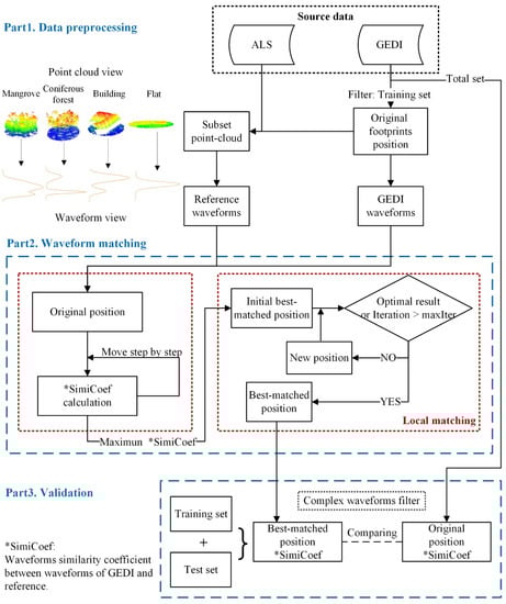
Figure 1.
The work flowchart of single temporal GEDI footprint position correction based on the waveform matching method.
2.1. Study Area
The study area included eight ALS collection areas with a total area of approximately 1461 km2, covering latitudes of 30° to 45°, longitudes of −122° to −81°, and elevations of 14–3776 m. The surface covering in the area mainly includes forests, shrubs, and grasslands without watershed and plant areas. The distribution of the study area is shown in Figure 2 and details are given in Table 1.
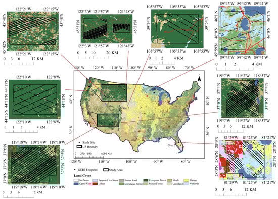
Figure 2.
The study sites’ (marked with black stars) distribution in this study. The background in the pictures is the 2019 land cover product from the National Land Cover Database (NLCD) [30] with a 12-class legend.

Table 1.
Airborne laser scanning (ALS) sites in the study.
2.2. Data Collection
2.2.1. GEDI Version 2 Product
GEDI collects global waveform LiDAR between 50°N and 50°S. The GEDI laser system contains three lasers and eight observation sample beams. GEDI scanning beams can be divided into strong and weak beams depending on the intensity of the laser energy. Depending on the requirements, GEDI offers different types of product, including raw transmitting and receiving waveforms (L1 product), ground height and canopy height at the footprint level (L2 product), and height and biomass data in grid form (L3 and L4 products). The available GEDI footprints within the study area can be obtained via GEDI Finder (https://git.earthdata.nasa.gov/projects/LPDUR/repos/GEDI-finder-tutorial-python/browse, accessed on 31 August 2022). The GEDI L1B [31] and L2B [32] products were used in this study, mainly for the real receiving waveforms and geographic location extraction, respectively. As each orbit has a unique orbit identifier (orbit number) in the GEDI footprint, GEDI temporal footprint IDs were determined using the ALS site name and orbit number in this study. The number of multi-temporal GEDI footprints used in this study is listed in Table 2 and shown in Figure 2.
Table 2.
Multi-temporal GEDI footprints with related attributes.
The value of the label “degrade_flag” was most relevant to the geolocation accuracy among all the attributes of GEDI footprints. The values of “degrade_flag” included non-zero and zero. The non-zero value had a corresponding orbital degradation situation of platform stability and GNSS position precision during operation. The “degrade_flag” label equaled zero, which means low probability with a certain two-degradation situation. The location accuracy may be better or worse in the surrounding periods near the beginning and end of the “degrade_flag” flagged intervals. Additionally, we considered the effects of different footprint acquisition times on geolocation error. The daytime/nighttime information was extracted from the attribute of “solar_elevation”. Additionally, we took the “sensitivity” label into account in the data pre-processing flow.
2.2.2. Airborne LiDAR Data
NEON is an ecological observation project (https://data.neonscience.org/data-products/explore, accessed on 31 August 2022). Among airborne data, airborne LiDAR data play an important role in quantitative information collection on land cover and changes in ecological structure.
The airborne laser scanning (ALS) data show centimeter-level ranging accuracy of 3D point-cloud data around the GEDI footprints. The ALS acquisition years were restricted to 2019, 2020, and 2021, with the average point densities across the sites varying from 8 to 60 points/m2, as determined using the scanner instrument Optech Gemini. The use of ALS and GEDI footprints from different years together was avoided in this study to prevent the influence of year-to-year physical variability in the experimental results. Table 1 presents all the ALS datasets used in this study, including spatial location, acquisition time (year-month), and elevation range [29].
Because the NEON onboard LiDAR platform is calibrated every winter, including horizontal and vertical positioning accuracy, the ALS data can be considered to be without geolocation error and can be used as a reference source for GEDI geolocation error correction. According to the data quality report, the vertical geolocation precision is generally less than 10 cm, and the horizontal geolocation precision is higher. ALS data were used for waveform simulation and correcting the footprint location by comparing the real waveform with the reference waveform, corresponding to part1 and part2 in the data processing flowchart (Figure 1).
2.3. Calculation of GEDI Footprints Geolocation Error using the Waveform Matching Method
The purpose of this study is to calculate the geolocation system error of temporal GEDI footprints and validate the correction result. Additionally, the main part of the evaluation of geolocation error was conducted using the GEDI Simulator.
The evaluation of GEDI footprint geolocation accuracy mainly included two main parts: reference waveform generation and error factor calculation. In the data pre-processing stage (Figure 1 part1), we selected the high-quality GEDI waveforms, mainly using the attributes of “sensitivity” and “quality” as the training set, for calculating the geolocation error.
The objective of reference waveform generation is to unify the form of reference data and GEDI observation data to facilitate data comparison. This process requires the real laser spot spatial position and ALS point-cloud data and converts the point-cloud data of the corresponding range of the ALS subset data into waveforms. The waveform simulation process has two main steps. The first step assigns the laser pulse energy within the footprint range according to a Gaussian distribution, and the weight of the horizontal position is assigned using the distance of each point in the point-cloud data relative to the center of the footprint. The parameters of the laser pulse are the same as those of the GEDI system. The second step is then convolved vertically to form a continuous waveform. Different land cover and longitudinal changes are often reflected in 3D point-cloud data with different point densities. In the different point density results in the formation of different waveform data, the waveform of the flat terrain area is monotonous with a single peak, while the area with complex terrain tends to generate a differently shaped waveform with multiple peaks. Additionally, greater changes in the point cloud cause greater changes in the waveform amplitude value, which tends to occur between the ground and above-ground objects.
The geolocation error is calculated by maximizing the average correlation coefficient between the GEDI waveforms and the reference waveforms as the waveform similarity coefficient (SimiCoef). SimiCoef is calculated from the denoised GEDI waveform G(t) and the reference waveform R(t), as in the following Equation (1):
where cov is the covariance of two curves, and σ is the standard deviation.
The calculation of the best-matched position is based on the criteria for maximizing the average SimiCoef value (Figure 3). The error calculation strategy used in this study was to carry out global matching first, and then, local matching. Firstly, we moved multiple GEDI footprints’ locations by a certain step and calculated the average SimiCoef matrix from the multiple SimiCoef matrixes of the footprints. In global matching, the moving step is an important factor affecting the matching result. On the one hand, too large a step will lead to low accuracy of the global matching result, thereby affecting the subsequent local matching accuracy result; on the other hand, too small a step calculation process is redundant and may cause program calculation failure due to limited computer resources. For a GLAS footprint with a ∼50 m diameter, the recommended step is 4 m [26]. In this study, the moving step was chosen to be 1 m, considering that the GEDI footprint diameter was 25 m.
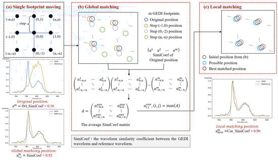
Figure 3.
The explanation of the process of calculating the best-matched position of GEDI footprints. Ori_SimiCoef and Cor_ SimiCoef present the SimiCoef of original and best-matched positions.
Then, the best position (i, j) of the globe matching serves as the initial position of the local matching. In the process of local optimization, the footprints’ positions are dynamically adjusted using the simplex optimization method [33]. The main idea of the simplex algorithm is to calculate the objective function to maximize SimiCoef, calculate the corresponding function value of the objective function at certain position, then sort the function value, and continuously iteratively replace the element with the smallest function value until the simplex converges near the maximum value of the function [34]. The algorithm calculation process is as follows:
- (1)
- Initialization: Determine the initial feasible basis and the initial feasible solution, and construct the initial simplex.
- (2)
- Optimality test: The coefficient of the non-basis variable is σ of the test number. If one of the following two conditions is met, the calculation is stopped and the current feasible solution is output as the optimal solution. Condition 1 is in the row corresponding to the objective function of the current table, all the values are non-positive, and Condition 2 is the number of iterations exceeding the pre-set threshold. Otherwise, go to the next step.
- (3)
- Convert from one feasible solution to another feasible solution with a larger target value and form a new simplex:
- Determine the variables that are swapped into the basis. Select > 0, the corresponding variable , as the substitution variable when there is more than one test number greater than 0 (generally, one should select the largest test number, that is, and its corresponding as the substitution variable.
- Identify swapped-out variables. Calculate and select θ according to Equation (2), and select the smallest corresponding basis variable as the swapped-out variable.where is the right-hand system item in the current table, and is the coefficient of the variable k in the ith constraint.
- Replace the swapped-out variable in the base variable with the swapped-in variable to obtain a new base. A new basis can be found for a new feasible solution, and a new simplex can be obtained accordingly.
- (4)
- Repeat steps 2 and 3 until the calculation is complete.
The best-matched footprint position is generated in two situations. Case 1 is where we obtain the optimal solution based on the judgment criteria of the simplex algorithm, while Case 2 is where the number of program iterations reaches the maximum and the last solution is considered the output [35]. In brief, globe matching tends to find the optimal result area and the best footprint location after local matching. Finally, we obtain the best-matched position through the system error coefficient in the x and y directions. The distance between the original and final positions is the geolocation error. Due to the characteristics of both brute-force search and local optimization, this experimental procedure can achieve centimeter-level positioning accuracy of horizontal geolocation.
2.4. The Validation of the Geolocation Error Position Correction
After evaluating the geolocation error of the GEDI footprints, we can correct the geolocation error using the system error coefficient. Additionally, we need to validate the correction result. We calculate and compare the average SimiCoef of the original and corrected locations.
The validation part consists of 4 steps. In Step 1, we filter complex GEDI waveforms by “mode” values greater than two considering that the waveform matching method is suitable for areas with complex terrain distribution. In Step 2, these complex waveforms are divided into a training set and a test set according to whether they are involved in the calculation of the geolocation or not. In Step 3, after converting the footprint’s spatial coordinates from the WGS84 geographic coordinate system to the local projection coordinate system, we apply the error distance in the x and y directions from Section 2.3. In the final step, we calculate the waveform similarity coefficients at the original position and the ideal position, respectively.
3. Results
3.1. Footprint Geolocation Accuracy of Multi-Temporal GEDI Footprints
To evaluate the geolocation deviation of the GEDI footprints, we calculated the geolocation error of different temporal GEDI footprints. The results of the geolocation error assessment of the GEDI (Table 3) explain the geolocation error calculated by the waveform matching method for the GEDI footprints. The error table includes the distance of the horizontal position system error, mainly in the X/Y direction. There are 22 Temporal GEDI footprints in total. The error distribution range is large (3.04–65.03 m) and relatively discrete, and about 72% (16/22) of the errors are concentrated between 3 m and 19 m. The difference between the median value (13.43 m) and the average value (20.91 m) of the error is 7.48 m.
Table 3.
The geolocation error distances of multi-temporal GEDI footprints.
The results of all the GEDI footprint corrections are stratified according to the GEDI footprint attribute “degrade_flag” value, separately for the good orbit and weak orbit parts, as shown in Table 4 (the good orbit means the temporal GEDI footprints are full of footprints with “degrade_flag” equal to 0; otherwise, the weak/degradation orbit is given). From Table 4 and Figure 4, the good orbit has a smaller error distance and a more concentrated distribution (9.46 m ± 3.83 m) than the weak orbit (30.45 m ± 21.22 m). By stratifying the GEDI footprint error results according to data time (night/day), the daytime GEDI footprint error distance tends to be larger, but both have a ratio of 3/12 (night) and 2/10 (day) with a large error (>30 m) in the temporal data. The error of nighttime footprints is more unstable, but the mean value is slightly less (night: 19.46 m ± 21.10 m, day: 22.68 m ± 15.98 m). Additionally, we find that the night and good orbit types account for 80% and 67% of the GEDI footprints with errors less than 13.43 m (the median value of multi-temporal GEDI footprints), while 20% and 33% of the large-error (error > 13.43 m) part respectively from Figure 4a. From Figure 4b, we find that the average values of the good orbit and nighttime GEDI footprint geolocation errors are smaller than the weak orbit and daytime errors, respectively.
Table 4.
The statistical geolocation error distance.
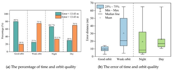
Figure 4.
The analysis of GEDI geolocation error is based on acquisition time (night/day) and orbit quality (good/weak). (a) The percentage of nighttime/daytime and good/weak orbit types of temporal GEDI footprints in two error groups; (b) the geolocation error distance distribution of four different conditions (including time and orbit quality).
3.2. The Correction of GEDI Footprint Geolocation Error
We use the best position from the waveform matching method to improve the geographic location of GEDI footprints. “SimiCoef” is the waveform similarity coefficient. “Ori_SimiCoef “ and “Cor_SimiCoef” represent the average of SimiCoef at the original and error-corrected positions, respectively, and “Perc_SimiCoef” is equal to . Figure 3 shows a typical example of the error correction with SimiCoef increasing.
The results show that Cor_SimiCoef is bigger than Ori_SimiCoef in all temporal GEDI footprints. To better discuss the improvement of the waveform matching correction effect, we divided all temporal GEDI datasets into two categories by Ori_SimiCoef. According to the Ori_SimiCoef value, C1 (<0.80) and C2 (>0.80) are generated with a threshold of 0.80. As shown in Figure 5, regardless of the Ori_SimiCoef value, the Cor_SimiCoef value increases. The improvement in the C1 dataset is greater than that in the C2 dataset, whether it is the Delta value (mean value: 0.10 > 0.02) or the ratio (mean value: 21.52 > 2.30). We believe the reason why there is a significant difference between these two types of data is mainly related to the Ori_SimiCoef. For GEDI footprints with high Ori_SimiCoef values, the waveform matching effect is good and the geolocation accuracy is relatively high, so it is difficult to greatly improve the SimiCoef. However, for footprints with a poor SimiCoef of the original position waveform, the waveform matching method can achieve a better matching effect.
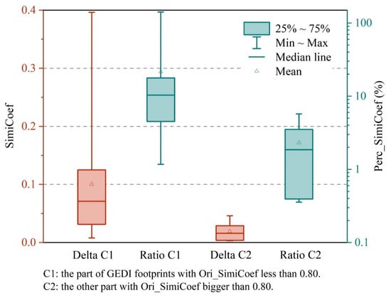
Figure 5.
The effect of SimiCoef (R) increasing after geolocation error correction in two GEDI sets (triangle is the mean value). C1 is the part of the GEDI footprints with Ori_SimiCoef less than 0.80 while C2 is the other part. Delta = Cor_SimiCoef-Ori_SimiCoef; Ratio = Delta/Ori_SimiCoef. Note that the vertical scale on the right has logarithmic distribution.
Table 5 shows the matching effects of different acquisition times and orbit qualities, respectively. For the GEDI footprints of weak orbit quality, the mean and median values (0.77 and 0.81, respectively) of the Cor_SimiCoef are lower than those of the GEDI footprints with all good orbit footprints (0.87 and 0.86), and the standard deviation of the weak orbit is larger than that of the good one (0.09 > 0.03) (Table 5). These indicate that the good orbit footprints have better accuracy of waveform matching at the original position and the correction method has better performance over weak orbit footprints. The Perc_SimiCoef values and standard deviations of the weak orbit are larger than the other, which means that the SimiCoef of the weak orbit rises higher than the other. Similarly, the waveform similarity of daytime GEDI footprints rises higher than the nighttime ones (mean value: 20.78 > 6.32), and its performance is more stable (std value: 8.75 < 40.55). Additionally, the Cor_SimiCoef of nighttime and daytime footprints is similar (0.82 and 0.81), but the ratio of SimiCoef increasing is different, indicating that the waveform matching method can improve the poor footprints to a better effect.
Table 5.
Waveform similarity coefficient (R) around orbit quality and data time.
The waveform matching effect cannot be guaranteed by simply increasing the SimiCoef value, and the waveform matching effect should also be defined by the SimiCoef value. We believe that when the average SimiCoef of the temporal GEDI footprints dataset is greater than a certain value, its matching works well. Otherwise, it is a poor match. We recorded the number of temporal GEDI footprints datasets that meet the threshold at the original and error-corrected position, respectively.
Different thresholds are shown in Table 6. The higher the SimiCoef threshold, the fewer the temporal GEDI footprint datasets with good waveform matching effects, both in the original position and the error-corrected position. Our waveform matching method can improve up to 32% (7/22) of all the temporal GEDI footprint datasets from poor matching results, corresponding to thresholds of 0.80 and 0.84. Coincidentally, the average GLAS SimiCoef value for the best-matched position in the forest scene is 0.801 [26], which is very close to the ‘optimal threshold’ mentioned above.
Table 6.
The different thresholds of waveform similarity coefficient (R) and the number of temporal GEDI footprint datasets that meet the threshold.
4. Discussion
4.1. The Correction Effect on Individual Footprints
Ideally, the correction result will make all footprints’ SimiCoef values increase after error correction. However, the average SimiCoef rising does not mean that the SimiCoef increases in every footprint. Therefore, we evaluated the correction effect on individual footprints by calculating the ratio of the increasing SimiCoef of individual waveforms as the credibility of the error correction result.
Table 7 describes all the used waveforms in the section. The geolocation error was calculated using the training set (part of the waveforms with high quality based on the “sensitivity” attribute), so the test set (the part of the waveforms not involved in the geolocation error calculation) could be used to validate the method. The number of sample complex waveforms involved in the calculation of the geolocation error was about 90% of the overall number of the region. All_valid_ratio, train_valid_ratio, and test_valid_ratio were used to represent the ratio of the increasing SimiCoef of individual waveforms after position correction. For all the GEDI footprints, the mean value and median of all_valid_ratio are 0.65 and 0.67, respectively. We consider the corrected position to be effective for 66% (the average of the mean value of 0.65 and the median of 0.67) of individual GEDI footprints.
Table 7.
The number of temporal GEDI footprints used in training and validation.
Figure 6 shows the distribution of three ratio values. It is important to know that the line at 50% is the split line for whether the waveform matching method works; when 50% of the individual footprints with Ori_SimiCoef are greater than Cor_SimiCoef, this means most individual waveform similarities are not improved, and the error-corrected positions are neither better nor worse. The median and mean values of all_valid_ratio, train_valid_ratio, and test_valid_ratio are similar, and the performance of the total set is close to that of the training set (Figure 6). However, the test set shows poor performance against the bigger variance of test_valid_ratio (the standard deviation of train_valid_ratio and test_valid_ratio is 0.09 and 0.17).
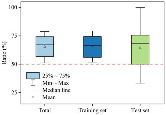
Figure 6.
The distribution of the ratio of the waveform similarity coefficient increases after error correction among the total GEDI footprints, training set, and test set. The triangle is the mean value. If the ratio is less than 50%, the correction effect is poor.
Therefore, the correct position can make the SimiCoef values of 66% of all laser waveforms increase, indicating effective improvement. Due to the large proportion (≈90%) of training sets used in this experiment, the poor performance of some test sets did not greatly affect the overall data performance.
The waveform matching method uses multiple waveforms to calculate the system error, but the effect on improving individual footprints’ waveform similarity in this study is effective for 66%. One reason for this situation is that the random error is not solved. One way to calculate the random error is to move one waveform at a time [23]. Future research can correct random errors after the system error is corrected.
4.2. The Limitations of the Waveform Matching Method
The waveform matching method is based on comparing the real receiving waveform with the reference waveform of spaceborne footprints and determining the best position using the maximum waveform similarity coefficient. As mentioned in the previous study, the “best-matched position” may not be the actual position due to factors such as the accuracy of the reference data, the waveform simulation method, etc. [26] The waveform simulation method has been widely used in the calibration of waveform processing algorithms for the GEDI mission and the quality assessment of the real receiving full waveform. This study used centimeter-level point-cloud data for reference waveform simulation, which greatly increases the credibility of the study findings.
However, some limitation factors should be addressed in future research.
Firstly, the waveform matching method is a statistical method in essence. The accuracy of the correct position is related to the training waveform selected and the point-cloud data point density. When selecting the training set, we only use a single threshold value in this study. Theoretically, the selected waveforms need to be representative, whether in waveform complexity or background noise, and follow a certain waveform sample selection ratio; a ratio too large or too small may lead to the calculation result not being ideal. Due to the difference in land cover type and flight altitude, the point density of reference point-cloud data varies from 9 to 60 points/m2. Low point density (<2 pts) may result in low ground elevation accuracy [28], but the influence on the waveform simulation is still unknown. How the two factors change the shape of the reference waveform requires further investigation.
Secondly, the method only considers the waveform of LiDAR without addressing the specific components of system error, which makes the correction result less convincing. In the process of spaceborne laser ground positioning, the accuracy of the laser pointing and the range error have a great influence on horizontal geolocation accuracy, and it is also an important part of the system error [11]. The terrain matching method has been used for ICESat-1/GLAS [22] and ICESat-2/ATLAS [7,36] system error correction, albeitwith rough accuracy. Additionally, the two-step geolocation error correction method of terrain waveform matching has been applied to a full-waveform laser altimeter GF-7 [37], and this new method corrects the 10 m system error. The combination of terrain and waveform matching on the GEDI footprint has great potential.
Thirdly, the acquisition time difference between GEDI and the reference data is one of the factors that causes non-matching results. In this study, the acquisition time of all the ALS datasets and multi-GEDI footprints is during a non-deciduous season, except at the MCRA site. At the MCRA site, we obtained ALS data in summer (2021-07) and MCRA16888 GEDI footprints in winter (2021-12). However, for the MCRA area of evergreen coniferous forest, seasonal differences do not cause a large difference in tree shape, and discrete-return LiDAR and waveform LiDAR have similar three-dimensional performance in winter coniferous forest mapping [38]. Even in snowy scenes, the different wavelengths of the two data sources (GEDI 532 nm and ALS 1064 nm) can only cause a 5% difference in receiving echo energy, and cannot change the matching effect to a large extent [39]. However, the waveform matching effect of broadleaf forest area has not been discussed in detail, especially the differences between deciduous and non-deciduous seasons.
5. Conclusions
The high geolocation quality of GEDI is a basic and important requirement for good data application, including forest height inversion and aboveground biomass estimation [40]. This study assesses the geolocation error of multi-temporal GEDI footprints using the method of waveform matching and validates the results of error correction. Overall, we mainly find some interesting results in the study. Firstly, the geolocation error of different temporal GEDI footprints ranges from 3.04 m to 65.03 m. The maximum is close to the GEDI orbit positioning accuracy of 60 m. Next, the good orbit quality performs better than the weak orbit, with an average value of 9.46 m, and the nighttime and daytime footprints perform similarly. Moreover, using 0.80 (or 0.84) as the threshold for measuring the matching effect, the waveform matching method can improve 32% of the temporal GEDI footprint datasets from poor matching. Additionally, in the validation part, waveform matching has a greater effect on low waveform similarity (waveform similarity coefficient value < 0.80) than high waveform similarity (>0.80). After system error correction of the individual footprints, about two-thirds of the waveform similarity improved, and the other third decreased.
We suggest that good-orbit-quality GEDI footprints should be preferred in future studies. As for acquisition time, nighttime GEDI data have been repeatedly proven to exhibit higher performance in height information extraction [41,42]. This mainly results from the low background noise of the waveform algorithm but it does not show a great effect on geolocation error. In a future study of geolocation error correction, we hope to study the influence of waveform sample selection and point-cloud point density on simulated waveforms; combine the terrain matching and waveform matching methods to improve the physical interpretation of system errors; increase the solutions to random errors; and explore the seasonal differences in matching effect in broadleaf forests.
Author Contributions
Conceptualization, Y.X. and H.H.; methodology, Y.X.; software, Y.X.; validation, Y.X.; formal analysis, Y.X., P.C. and H.H.; investigation, Y.X.; funding acquisition, S.D.; writing—original draft preparation, Y.X.; writing—review and editing, Y.X., S.D., P.C., H.H., H.T. and H.R.; visualization, Y.X. and P.C. All authors have read and agreed to the published version of the manuscript.
Funding
This research was supported by the Scientific and Technological Innovation Project for Forestry in Guangdong (2022KJCX004), the Open Research Program of the International Research Center of Big Data for Sustainable Development Goals (CBAS2022ORP04), and the Major Key Project of PCL.
Data Availability Statement
Publicly available datasets were analyzed in this study. These data can be found at https://search.earthdata.nasa.gov/search?q=GEDI (accessed on 28 August 2021) and https://data.neonscience.org/data-products/explore (accessed on 28 August 2021).
Acknowledgments
The authors acknowledge the support of the GEDI Mission Team and the NEON project for providing the GEDI and ALS datasets, respectively. We would also like to thank Steven Hancock, who provided the initial instructions for using the GEDI Simulator.
Conflicts of Interest
The authors declare no conflict of interest. The funders had no role in the design of the study; in the collection, analyses, or interpretation of the data; in the writing of the manuscript; or in the decision to publish the results.
References
- Salas, E.A.L. Waveform LiDAR concepts and applications for potential vegetation phenology monitoring and modeling: A comprehensive review. Geo-Spat. Inf. Sci. 2021, 24, 179–200. [Google Scholar] [CrossRef]
- Li, X.; Liu, C.; Wang, Z.; Xie, X.; Li, D.; Xu, L. Airborne LiDAR: State-of-the-art of system design, technology and application. Meas. Sci. Technol. 2021, 32, 32002. [Google Scholar] [CrossRef]
- Chen, Q. Assessment of terrain elevation derived from satellite laser altimetry over mountainous forest areas using airborne LiDAR data. ISPRS-J. Photogramm. Remote Sens. 2010, 65, 111–122. [Google Scholar] [CrossRef]
- Qin, R.; Tian, J.; Reinartz, P. 3d change detection–approaches and applications. ISPRS J. Photogramm. Remote Sens. 2016, 122, 41–56. [Google Scholar] [CrossRef]
- Magruder, L.A.; Webb, C.E.; Urban, T.J.; Silverberg, E.C.; Schutz, B.E. ICESat altimetry data product verification at white sands space harbor. IEEE Trans. Geosci. Remote Sens. 2007, 45, 147–155. [Google Scholar] [CrossRef]
- Dubayah, R.; Blair, J.B.; Goetz, S.; Fatoyinbo, L.; Silva, C. The global ecosystem dynamics investigation: High-resolution laser ranging of the earth’s forests and topography. Sci. Remote Sens. 2020, 1, 100002. [Google Scholar] [CrossRef]
- Zhao, P.; Li, S.; Ma, Y.; Liu, X.; Yang, J.; Yu, D. A new terrain matching method for estimating laser pointing and ranging systematic biases for spaceborne photon-counting laser altimeters. ISPRS J. Photogramm. Remote Sens. 2022, 188, 220–236. [Google Scholar] [CrossRef]
- Fraccaro, P.; Beukenhorst, A.; Sperrin, M.; Harper, S.; Palmier-Claus, J.; Lewis, S.; Van der Veer, S.N.; Peek, N. Digital biomarkers from geolocation data in bipolar disorder and schizophrenia: A systematic review. J. Am. Med. Inf. Assoc. 2019, 26, 1412–1420. [Google Scholar] [CrossRef]
- Beck, J.; Wirt, B.; Luthcke, S.B.; Hofton, M.; Armston, J. Global Ecosystem Dynamics Investigation (GEDI) Level 1b User Guide; U.S. Geological Survey (USGS) Earth Resources Observation and Science (EROS) Center: Sioux Falls, SD, USA, 2020. Available online: https://lpdaac.usgs.gov/documents/987/GEDI01B_User_Guide_V2.pdf (accessed on 10 August 2022).
- Fan, C.; Li, J.; Wang, D.; Zhang, Y.; Shi, X. ICESat/glas laser footprint geolocation and error analysis. J. Geod. Geodyn. 2007, 27, 104–106. [Google Scholar]
- Yue, C.; He, H.; Bao, Y.; Xing, K.; Zhou, N. Error propagation of exterior orientation elements study on space-borne laser altimeter ground positioning. In Proceedings of the Conference on Lidar Technologies, Techniques, and Measurements for Atmospheric Remote Sensing X, Amsterdam, The Netherlands, 22–25 September 2014; Singh, U.N., Pappalardo, G., Eds.; Volume 9246. [Google Scholar]
- Schutz, B.E.; Zwally, H.J.; Shuman, C.A.; Hancock, D.; Dimarzio, J.P. Overview of the ICESat mission. Geophys. Res. Lett. 2005, 32, L21S01. [Google Scholar] [CrossRef]
- Eegholm, B.; Wake, S.; Denny, Z.; Dogoda, P.; Poulios, D.; Coyle, B.; Mulé, P.; Hagopian, J.; Thompson, P.; Ramos-Izquierdo, L.; et al. Global ecosystem dynamics investigation (GEDI) instrument alignment and test. Opt. Model. Syst. Alignment 2019, 11103, 1110308. [Google Scholar]
- Schultz, C.J.; Lang, T.J.; Leake, S.; Runco, M.; Stefanov, W. A technique for automated detection of lightning in images and video from the international space station for scientific understanding and validation. Earth Space Sci. 2021, 8, e2020EA001085. [Google Scholar] [CrossRef]
- Leake, S. Reverse geolocation of images taken from the international space station utilizing various lightning datasets. In Proceedings of the IEEE Aerospace Conference, Big Sky, MT, USA, 2–9 March 2019; p. 10. [Google Scholar]
- Guo, H.; Dou, C.; Zhang, X.; Han, C.; Yue, X. Earth observation from the manned low earth orbit platforms. ISPRS J. Photogramm. Remote Sens. 2016, 115, 103–118. [Google Scholar] [CrossRef]
- Montenbruck, O.; Rozkov, S.; Semenov, A.; Gomez, S.F.; Nasca, R.; Cacciapuoti, L. Orbit determination and prediction of the international space station. J. Spacecr. Rockets 2011, 48, 1055–1067. [Google Scholar] [CrossRef]
- Dou, C.; Zhang, X.; Kim, H.; Ranganathan, J.; Olsen, D.; Guo, H. Geolocation algorithm for earth observation sensors onboard the international space station. Photogramm. Eng. Remote Sens. 2013, 79, 625–637. [Google Scholar] [CrossRef]
- Dou, C.; Zhang, X.; Guo, H.; Han, C.; Liu, M. Improving the geolocation algorithm for sensors onboard the iss: Effect of drift angle. Remote Sens. 2014, 6, 4647–4659. [Google Scholar] [CrossRef]
- Luthcke, S.B.; Rowlands, D.D.; Mccarthy, J.J.; Pavlis, D.E.; Stoneking, E. Spaceborne laser-altimeter-pointing bias calibration from range residual analysis. J. Spacecr. Rocket. 2000, 37, 374–384. [Google Scholar] [CrossRef]
- Sirota, J.M.; Bae, S.; Millar, P.; Mostofi, D.; Webb, C.; Schutz, B.; Luthcke, S. The transmitter pointing determination in the geoscience laser altimeter system. Geophys. Res. Lett. 2005, 32, 1–18. [Google Scholar] [CrossRef]
- Filin, S. Calibration of spaceborne laser altimeters-an algorithm and the site selection problem. IEEE Trans. Geosci. Remote Sens. 2006, 44, 1484–1492. [Google Scholar] [CrossRef]
- Schleich, A.; Soma, M.; Durrieu, S.; Véga, C.; Renaud, J.P.; Bouriaud, O. Improving GEDI footprint geolocation using a high resolution digital terrain model. In Proceedings of the SilviLaser Conference, Vienna, Austria, 28–30 September 2021; pp. 179–181. [Google Scholar]
- Harding, D.J. ICESat waveform measurements of within-footprint topographic relief and vegetation vertical structure. Geophys. Res. Lett. 2005, 32. [Google Scholar] [CrossRef]
- Chunyu, Y.; Kun, X.; Yunfei, B.; Nan, Z. A matching method of space-borne laser altimeter big footprint waveform and terrain based on cross cumulative residual entropy. Acta Geod. Cart. Sin. 2017, 46, 346–352. [Google Scholar]
- Wang, C.; Yang, X.; Xi, X.; Zhang, H.; Chen, S.; Peng, S.; Zhu, X. Evaluation of footprint horizontal geolocation accuracy of spaceborne full-waveform LiDAR based on digital surface model. IEEE J. Sel. Top. Appl. Earth Observ. Remote Sens. 2020, 13, 2135–2144. [Google Scholar] [CrossRef]
- Hancock, S.; Armston, J.; Hofton, M.; Sun, X.; Tang, H.; Duncanson, L.I.; Kellner, J.R.; Dubayah, R. The GEDI simulator: A large-footprint waveform LiDAR simulator for calibration and validation of spaceborne missions. Earth Space Sci. 2019, 6, 294–310. [Google Scholar] [CrossRef]
- Huettermann, S.; Jones, S.; Soto-Berelov, M.; Hislop, S. Intercomparison of real and simulated GEDI observations across sclerophyll forests. Remote Sens. 2022, 14, 2096. [Google Scholar] [CrossRef]
- NEON (National Ecological Observatory Network). Discrete Return LiDAR Point Cloud (DP1.30003.001). Available online: https://data.neonscience.org (accessed on 31 August 2022).
- Dewitz, J.U.S. Geological Survey 2021, National Land Cover Database (NLCD) 2019 Products (ver. 2.0, June 2021) [Data Set]. U.S. Geological Survey: Sioux Falls, SD, USA; 2021. Available online: https://data.usgs.gov/datacatalog/data/USGS:60cb3da7d34e86b938a30cb9 (accessed on 31 August 2022).
- Dubayah, R.; Luthcke, S.; Blair, J.B.; Hofton, M.; Armston, J.; Tang, H. GEDI L1B Geolocated Waveform Data Global Footprint Level V002 [Data Set]. NASA EOSDIS Land Processes DAAC; 2020. Available online: https://lpdaac.usgs.gov/products/gedi01_bv002/ (accessed on 31 August 2022).
- Dubayah, R.; Tang, H.; Armston, J.; Luthcke, S.; Hofton, M.; Blair, J.B. GEDI L2B Canopy Cover and Vertical Profile Metrics Data Global Footprint Level V002 [Data Set]. NASA EOSDIS Land Processes DAAC; 2021. Available online: https://lpdaac.usgs.gov/products/gedi02_bv002/ (accessed on 31 August 2022).
- Press, W.H.; Teukolsky, S.A.; Vetterling, W.T.; Flannery, B.P. Numerical Recipes in C, 2nd ed.; Cambridge Univ. Press: Cambridge, UK, 1994. [Google Scholar]
- Gao, F.; Han, L. Implementing the nelder-mead simplex algorithm with adaptive parameters. Comput. Optim. Appl. 2012, 51, 259–277. [Google Scholar] [CrossRef]
- Wen, G.; Li, D.; Yuan, X. A global optimal registration method for satellite remote sensing images. Int. Arch. Photogramm. Remote Sens. Spat. Inf. Sci. 2002, 34, 394–399. [Google Scholar]
- Schenk, T.; Csatho, B.; Neumann, T. Assessment of ICESat-2’s horizontal accuracy using precisely surveyed terrains in mcmurdo dry valleys, antarctica. IEEE Trans. Geosci. Remote Sens. 2022, 60, 1–11. [Google Scholar] [CrossRef]
- Li, G.; Tang, X.; Zhou, X.; Lu, G.; Chen, J.; Huang, G.; Gao, X.; Liu, Z.; Ouyang, S. The method of gf-7 satellite laser altimeter on-orbit geometric calibration without field site. Acta Geod. Cartogr. Sin. 2022, 51, 401–412. [Google Scholar]
- Chhatkuli, S.; Mano, K.; Kogure, T.; Tachibana, K.; Shimamura, H.; Shortis, M.; Wagner, W.; Hyyppa, J. Full waveform LiDAR exploitation technique and its evaluation in the mixed forest hilly region. In Proceedings of the XXII ISPRS CONGRESS, TECHNICAL COMMISSION VII: 22nd Congress of the International-Society-for-Photogrammetry-and-Remote-Sensing, Melbourne, Australia, 25 August–1 September 2012; Volume 39, pp. 505–509. [Google Scholar]
- Deems, J.S.; Painter, T.H.; Finnegan, D.C. Lidar measurement of snow depth: A review. J. Glaciol. 2013, 59, 467–479. [Google Scholar] [CrossRef]
- Saarela, S.; Holm, S.; Healey, S.P.; Patterson, P.L.; Yang, Z.; Andersen, H.; Dubayah, R.O.; Qi, W.; Duncanson, L.I.; Armston, J.D.; et al. Comparing frameworks for biomass prediction for the global ecosystem dynamics investigation. Remote Sens. Environ. 2022, 278, 113074. [Google Scholar] [CrossRef]
- Potapov, P.; Li, X.; Hernandez-Serna, A.; Tyukavina, A.; Hansen, M.C.; Kommareddy, A.; Pickens, A.; Turubanova, S.; Tang, H.; Silva, C.E.; et al. Mapping global forest canopy height through integration of GEDI and landsat data. Remote Sens. Environ. 2021, 253, 112–165. [Google Scholar] [CrossRef]
- Liu, A.; Cheng, X.; Chen, Z. Performance evaluation of GEDI and ICESat-2 laser altimeter data for terrain and canopy height retrievals. Remote Sens. Environ. 2021, 264, 112571. [Google Scholar] [CrossRef]
Disclaimer/Publisher’s Note: The statements, opinions and data contained in all publications are solely those of the individual author(s) and contributor(s) and not of MDPI and/or the editor(s). MDPI and/or the editor(s) disclaim responsibility for any injury to people or property resulting from any ideas, methods, instructions or products referred to in the content. |
© 2023 by the authors. Licensee MDPI, Basel, Switzerland. This article is an open access article distributed under the terms and conditions of the Creative Commons Attribution (CC BY) license (https://creativecommons.org/licenses/by/4.0/).