A Novel Deep Nearest Neighbor Neural Network for Few-Shot Remote Sensing Image Scene Classification

Abstract

Remote sensing image scene classification has become more and more popular in recent years. As we all know, it is very difficult and time-consuming to obtain a large number of manually labeled remote sensing images. Therefore, few-shot scene classification of remote sensing images has become an urgent and important research task. Fortunately, the recently proposed deep nearest neighbor neural network (DN4) has made a breakthrough in few-shot classification. However, due to the complex background in remote sensing images, DN4 is easily affected by irrelevant local features, so DN4 cannot be directly applied in remote sensing images. For this reason, a deep nearest neighbor neural network based on attention mechanism (DN4AM) is proposed to solve the few-shot scene classification task of remote sensing images in this paper. Scene class-related attention maps are used in our method to reduce interference from scene-semantic irrelevant objects to improve the classification accuracy. Three remote sensing image datasets are used to verify the performance of our method. Compared with several state-of-the-art methods, including MatchingNet, RelationNet, MAML, Meta-SGD and DN4, our method achieves promising results in the few-shot scene classification of remote sensing images.

1. Introduction

Remote sensing is a detection technology used to obtain target information from a long distance [1,2,3]. With the rapid development of remote sensing technology, remote sensing images play an increasingly important role in both military and civilian fields [4,5,6]. On the basis of image content, each remote sensing image is divided into different classes in a scene classification task [7,8,9], which is an important means to understand remote sensing images. It is applied to natural disaster detection [10,11], urban planning [12,13], environmental monitoring [14,15], vegetation mapping [16], land cover analysis [17] and other fields.

Handcrafted features play an important role in the early study of scene classification, such as SIFT [18], color histograms [19], HOG [20] and GIST [21]. These methods usually concentrate on utilizing significant engineering tricks and domain professionals to model different handcrafted features, such as color, spectral, shape, and spatial information, or combinations of them, which are the dominant features of scene images, and therefore are helpful for scene classification.

Unsupervised feature learning has attracted the attention of many scholars and made great progress in the field of remote sensing image classification in recent years, such as autoencoder [22] and sparse coding [23]. Unsupervised feature learning is designed to learn a series of basis functions for feature coding, where a series of handcrafted features or the original feature of the image is input into the function and the unsupervised learned features are output.

Recently, deep learning methods have achieved encouraging results in remote sensing image scene classification tasks [24], such as VGG16 [25], ResNet [26], AlexNet [27] and GoogLeNet [28]. However, these excellent methods rely heavily on a large number of labeled training samples. In practical applications, due to the particularity of remote sensing images, it is very difficult and time-consuming to obtain a large number of manually labeled high-resolution remote sensing images, especially for special scenes such as military facilities (such as missile positions and military areas) [29]. Once the available labeled data are insufficient, the deep learning method will have the risk of over-fitting, which will lead to performance degradation. Therefore, the scene classification of remote sensing images has become an urgent and important research task in the case of few labeled samples. In addition, most of the existing classification methods based on deep neural networks can only classify the trained scenes. If the new scene class is not in the class list of the training dataset, it is difficult for the deep learning method to classify it. When the deep learning model is used to identify the new scene that does not appear in the training dataset, a large number of labeled samples of the new scene class need to be collected again, and the classification model needs to be retrained to avoid catastrophic forgetting, which will lead to consuming time and computing resources.

To solve the above problems, a few-shot learning method is often used to classify invisible classes without retraining the entire model, and some scholars have also applied few-shot learning to remote sensing image scene classification [4,30,31]. Few-shot learning is a new research direction inspired by humans’ fast learning ability, which enables machine vision systems to quickly learn new tasks from limited labeled data. Recently, some researchers have used few-shot learning to reduce the burden of data annotation, and improve the generalization ability of the model for new classes with only a few labeled samples. Few-shot learning has been successfully applied to computer vision, natural language processing, speech recognition, medical image classification and other tasks [32]. Few-shot remote sensing image scene classification is also a promising field still at an early stage. The few-shot scene classification network can directly classify the new scenes that do not exist in the training set, saving the cost of marking images and retraining.

However, the existing few-shot image classification networks are usually applied to natural images, and the difference between remote sensing images and natural images is very significant. Since remote sensing images are shot from a bird’s-eye view, they inevitably contain objects unrelated to the semantic class of the scene, which will cause adverse interference to the classification performance. For the classification of a basketball court in the upper left corner of Figure 1, the main target object is the basketball court, but there are also some unrelated objects in the image, such as cars, buildings and plants. Similar situations also occur in other scenes such as roundabouts, ground track fields, and freeways.

In the metric-based few-shot learning method, the deep nearest neighbor neural network (DN4) [33] is one of the most advanced algorithms. Few-shot learning methods based on metric-learning mainly depend on learning an informative similarity metric. These methods mainly use image-level features for classification. However, image-level features under a few-shot conditions are often sparse, and some discrimination information will be lost. This loss is often irreversible, leading to poor classification performance. Compared with image-to-image metrics in some few-shot learning methods, the deep local descriptors and image-to-class metric are used in DN4, motivated by naive–Bayes nearest-neighbor (NBNN) [34], to directly calculate the distance between the descriptor of the query image and the class, effectively reducing the quantization error. DN4 has made a breakthrough in few-shot learning, but due to the complex background in remote sensing images, the model is easily affected by irrelevant local features, so the model cannot be directly applied in remote sensing images. Therefore, it is necessary to introduce the attention mechanism, which can give the relevant local features a higher weight and give the irrelevant local features a lower weight. In this way, the impact of the irrelevant local features can be reduced.

In this paper, a deep nearest neighbor neural network based on attention mechanism (DN4AM) is proposed to realize the end-to-end framework of few-shot remote sensing image scene classification. There are three main innovations of our method. Firstly, our method introduces an episodic training method to train the network and tests on the new class for few-shot learning. Secondly, our method designs the scene class-related attention map through the channel attention mechanism with global information to suppress the influence of irrelevant regions. Lastly, the similarities of the local descriptors between the query image and the class image are weighted by a scene class-related attention map, which finally obtains the image-to-class metric score, which is meaningful for reducing interference from scene-semantic irrelevant objects to improve classification accuracy. Section 2 gives the related work. Our proposed method is presented in Section 3. Section 4 gives the experimental results and analysis. Finally, conclusions are drawn in Section 5.

2. Related Work

2.1. Few-Shot Scene Classification of Remote Sensing Images

Different from traditional supervised learning methods, few-shot learning cannot acquire comprehensive prior knowledge due to having less labeled samples. Therefore, the knowledge transfer of the same class sample and internal relationship learning become important in the few-shot scene classification of remote sensing images. Vin proposed an episodic training method [35]. During the training process, C classes are randomly selected from the auxiliary dataset, and K images are randomly sampled from each class. $C\times K$ images constitute the support set of the few-shot task. At the same time, in the remaining images of the C classes, a number of samples are randomly selected in equal quantities for each class to form a query set to assist the few-shot classification task. An episode consists of a support set and a query set. Several episodes are iterated until the loss value of the network converges, and the network is finally used to test the classification accuracy of the actual few-shot task. Due to the case that a support set has C classes and K samples for each class in the episodic training, it is also known as the C-way K-shot problem. The advantage of this training method is that the network can learn to learn, and make the network generalization performance better. The changing tasks make the network learn how to adapt to new few-shot tasks, which is more suitable for a few-shot learning case.

The few-shot scene classification of remote sensing images can be regarded as a series of C-way K-shot problems, and the overall dataset can be divided into a training dataset, validation set and testing dataset, and no overlap of the label space of the three subsets. The experimental procedure consists of the training, validation, and testing processes, as described below.

During the training process, multiple episodes are obtained from the training dataset randomly. The process of episode construction is as follows:

(1) C classes are randomly selected from the training dataset, with K samples for each class, and the sample set extracted is used as the support set $S=\left\{\left(s_i,y_i\right)\mid i=1,\cdots ,C\times K\right\}$, where $s_i$ represents the ith sample of the support set, and $y_i$ represents the corresponding label.

(2) In the remaining samples, N samples are also randomly selected for each class in the support set, and the corresponding query set $Q=\left\{\left(q_j,{\tilde{y}}_j\right)\mid j=1,\cdots ,C\times N\right\}$ is obtained, where $q_j$ and ${\tilde{y}}_j$ represent the jth sample and label in the query set, respectively. There is no intersection between the support set and the query set, that is $S\cap Q=⌀$.

A support set and a query set form an episode. In an iterative process of the training stage, the episode is extracted from the training dataset as the input data for forward propagation, and the network parameters are updated by the gradient descent of the loss function, eventually learning a well-trained model.

The validation process and the testing process use the episode in a similar way to the training process. Both the support set and the query set are sampled from the validation dataset or the testing dataset. The model is trained for forward propagation to predict the labels of the query set based on the support set. The difference is that the main purpose of the validation process is to select suitable hyperparameters for the model, and the results of the testing dataset are used to evaluate the performance of the model.

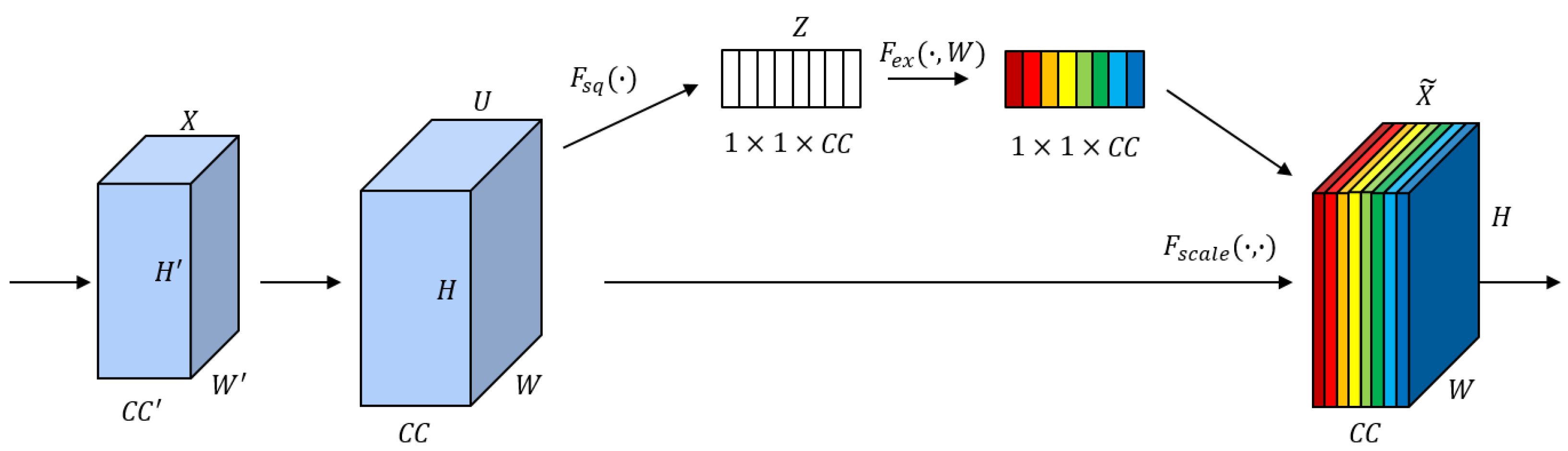
2.2. Channel Attention Mechanism

There are several convolutional cores in convolutional layer of convolutional neural networks (CNN), so the generated feature map will have multiple channels, each channel reflects the corresponding situation of a feature, but not all features have the same importance to the final task. The researchers began to study another aspect of network architecture design, namely the attention mechanism, also known as feature recalibration. In the convolutional layer of the model, the attention mechanism can not only guide these convolutional layers to see where the image looks at, but also to improve the feature representation of the region of interest by focusing on important features and suppressing less-useful features. The attention mechanism can increase the feature representation capability of the network by clearly modeling the interdependence between the channels and spaces of feature maps by adding a few network parameters. Hu et al. [36] designed an architecture based on the channel attention mechanism, namely Squeeze-and-Excitation (SE), a module that focuses on the dependencies between the channels. The structure of the SE module is shown in Figure 2.

Given a feature map of $H\times W\times CC$ size, the SE module first presses the input feature map to $1\times 1\times CC$ size by a squeeze operation, which can be expressed as:

$$\begin{array}{cc}\hfill & z_{cc}=\frac{1}{H\times W}\sum _{i=1}^H\sum _{j=1}^W{u}_{cc}(i,j)\hfill \end{array}$$

(1)

where H and W, respectively, represent the height and width size of the feature map, and $u_{cc}(i,j)$ represents the response value of the $cc$th channel of the feature map at $(x,y)$.

The excitation operation contains two fully connected layers and two nonlinear activation layers, which can be represented as:

$$\begin{array}{cc}\hfill & z_s=\sigma \left(W_2\delta \left(W_{1}z\right)\right)\hfill \end{array}$$

(2)

where $W_1$ and $W_2$ are the weights of the fully connected layers, $\delta$ and $\sigma$ represent the ReLU activation function and the Sigmoid activation function, respectively. The first fully connected layer reduces the channel dimension of the input feature in a certain proportion, and adopts the ReLU activation function, while the last fully connected layer is used to recover the channel dimension, and uses the Sigmoid function for nonlinear activation. The final output of the SE module is obtained by the dot product of the activation value and the input features.

2.3. Deep Nearest Neighbor Neural Network

Few-shot image classification refers to learning a classifier to classify images when there are few training samples for each class. Recently, some studies have achieved good classification performance on few-shot natural images, in which an image-level feature-based metric is usually used. Li et al. [33] believe that the image-level feature representation obtained through the current few-shot learning methods may lose a lot of discrimination information, and this loss is not recoverable and leads to poor performance of the few-shot classification. Therefore, Li et al. [33] proposed the DN4 network, which is mainly composed of a deep embedding module and an image-to-class (I2C) module. These two modules are briefly described below.

The deep embedding module in DN4 is used to learn the feature representation of the image. If a given set of support and query images is input, the deep embedding module outputs the corresponding deep local descriptors for the subsequent metric process. In theory, the CNN module can be utilized as a deep embedding module, as long as the CNN module can learn image features. In order to facilitate the comparison with other methods, the Conv-64F network commonly used in few-shot learning is adopted in DN4. This network has only four convolutional blocks, each of which consists of 64 convolutional blocks with a size of $3\times 3$ convolutional filter, batch normalization layer and leaky ReLU activation layer. Additionally, this network also adds a $2\times 2$ max pooling layer after the first two convolutional blocks for down-sampling operation. Given an image X and input module $\mathrm{\Psi }$, the output $\mathrm{\Psi }\left(X\right)$ will be a tensor of size $h\times w\times d$ that can be regarded as a set of q deep local descriptors of d dimension, where $q=h\times w$, and w, h, and d represent the width, height, and number of channels of the feature map, respectively.

The I2C module constructs a local descriptor space for a class using deep local descriptors from all the support set images in the class. In this space, the module calculates the distance between the query image and the class through k-nearest neighbors (kNN) [37], that is, the similarity between the image and the class. Compared with the image-level feature, the image-to-class metric is used in DN4 to directly calculate the distance between the deep local descriptors of the query image and the whole class, which effectively reduces the quantization error. The KNN algorithm used in the I2C module is a nonparametric classification technology based on analogy learning, and the training process is simple and rapid, which can avoid the problem of an unbalanced sample number. It is noteworthy that the I2C module can effectively prevent overfitting caused by parameter learning.

Specifically, due to the small number of samples for few-shot learning, Li et al. [33] believe that an image-to-class metric based on the local descriptors should be adopted, that is, the DN4 model is proposed on the basis of the latest episodic training mechanism and is trained end-to-end. The key difference between DN4 and the few-shot learning method using an image-level feature metric is that the image-to-class metric based on local descriptors is used in the last layer of DN4, and this metric is realized through a KNN search of the deep local descriptors of the convolutional feature maps. The proposed DN4 not only learns the optimal deep local descriptors of image-to-class metric, but also utilizes the interchangeability of visual patterns between images in the same class with fewer samples, that is, a new image can be composed by using image blocks of other images in the same class. The DN4 model provides a simple, effective and computationally efficient framework for learning with fewer samples. It has made a breakthrough in few-shot learning, but it also has some shortcomings that need to be solved. On the one hand, like other state-of-the-art few-shot learning models, DN4 mainly uses Softmax loss to force distance between different classes of deep features, but ignores the compactness within the class. On the other hand, due to the complex background in remote sensing image scene classification, DN4 is easily affected by irrelevant local features.

3. Methods

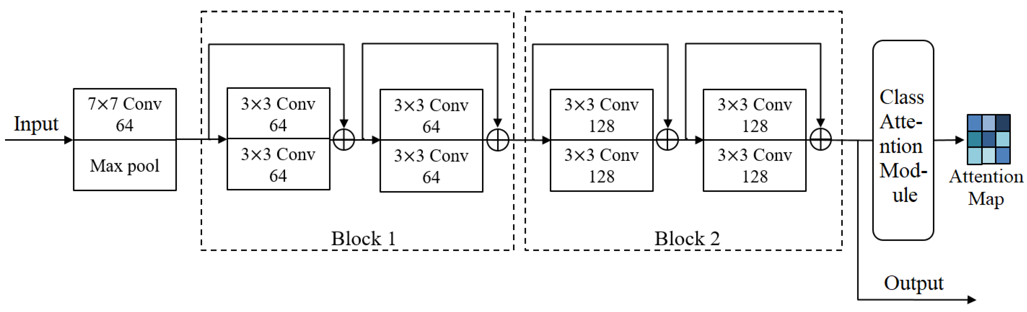
3.1. Architecture

In order to solve the problem that few-shot scene classification is prone to irrelevant background noise interference due to the complex background in remote sensing images, DN4AM is proposed in this paper, which consists of two modules: attention-based deep embedding module and metric module.

The architecture of DN4AM is shown in Figure 3, which inputs the support image and query image of each class into the network. The attention-based deep embedding module $f_{\psi }(·)$ can learn the deep local descriptors of all images and the attention maps related to the scene class. Similar to DN4, the sample q in query set Q and the sample s in support set S pass through the embedding module $f_{\psi }(·)$ to output the corresponding feature maps $f_{\psi }\left(q\right)$ and $f_{\psi }\left(s\right)$. For each image $XX$, $f_{\psi }\left(XX\right)$ is a feature map of size $h\times w\times d$, which can be regarded as a $h\times w$ set of d-dimensional local descriptors. It is worth noting that the class-related attention learning module is introduced into the embedding module. By clustering, weighting and pooling the feature channels to generate the attention feature map, the deep local descriptors are divided into the relevant part of the scene and the irrelevant part of the background, thus weakening the irrelevant features and effectively reducing the background noise. Finally, the similarity of the local descriptors between the query image and the class image is measured through the metric module $f_{\phi }(·)$, and the weighted sum is made using the attention map as the final output of prediction probability value.

Both the first convolutional layer and the first two convolutional blocks of ResNet18 [26] are utilized as the deep embedding module in our method. Some few-shot learning methods use the four-layer shallow network Conv-64F to avoid over-fitting, but Chen et al. found that when the domain difference between the new class and the base class is very small, using a deeper backbone network can significantly improve the performance [38]. Remote sensing images are relatively similar, unlike natural images that have a large domain difference. Therefore, in this paper, we attempt to extract the discriminative features using deeper networks. The final experimental results also show that ResNet18 has better performance than the four-layer shallow backbone network.

3.2. Attention-Based Deep Embedding Module

Module $f_{\psi }(·)$ is used to learn the deep local features of the query images and the support images, and any appropriate CNN model can be used as a deep embedding module. The first convolutional layer and the first two convolutional blocks of ResNet18 are used as the deep embedding module, as shown in Figure 4. Each convolutional block is composed of four $3\times 3$ convolutional filters. The number of channels of the first convolutional block is 64, and the number of channels of the second convolutional block is 128. A jump connection operation is added after every two convolutional layers. Given an input image $XX$, the deep feature extracted by the embedding module can be expressed as $f_{\psi }\left(XX\right)$, which is essentially a tensor with a size of $h\times w\times d$, where w, h, and d, respectively, represent the width, height and number of channels of the feature map. In this paper, they are regarded as a set of m d-dimensional deep local descriptors, namely:

$$\begin{array}{cc}\hfill & f_{\phi }\left(XX\right)=\left[x_1,x_2,\dots ,x_m\right]\in R^{d\times m}\hfill \end{array}$$

(3)

where $m=h\times w$, and $x_i$ is the ith deep local descriptor. Suppose an image has a resolution of $224\times 224$, the output feature map is $h=w=28$, $d=128$, which means that each image has a total of 784 deep local descriptors. Local features can offer information that can be distinguished and transferred across classes, which may be an important clue for image classification in few-shot scenes. An ideal metric-based method should be able to take advantage of local information and minimize the interference caused by unrelated regions. Therefore, our method introduces the attention mechanism in the deep embedding module, which divides the deep local descriptors into the relevant part of the scene and the irrelevant part of the background.

Convolutional feature channels can correspond to specific types of visual patterns, and multiple channels can express rich information. In the convolutional layer of the network model, the attention mechanism can guide which areas of the image these convolutional layers focus on, and explicitly model the interdependencies between feature map channels and spaces. Therefore, adding an attention mechanism in the deep embedding module to divide the different channels into the part related to the scene class and the part unrelated to the scene class is considered. The SE module is a common channel attention mechanism, which uses the squeeze operation to obtain a global information statistic and the excitation operations to model the interdependencies between feature channels. The SE module usually obtains the global information statistic through a global average pooling (GAP) [39] operation, but not all local image areas are equally representative to describe the target objects in the image. In addition, the existing GAP strategy does not process the spatial information, so that each local descriptor has the same importance, which not only leads to the loss of information, but also prevents the learner from paying attention to the image area with important information, leading to a negative impact on the classifier. Wang et al. [40] proposed the non-local attention module, which can capture the long-distance dependence in the deep neural network by constructing an attention feature map for each pixel of the feature map.

Based on the study of the SE module and the non-local attention mechanism, we design a class-related attention module, in which a non-local attention mechanism is used instead of the GAP operation. As shown in Figure 5, the non-local attention module for the global information statistics operation is utilized in the class-related attention module, and the global attention feature map from the Softmax function is summed as a weighted value. The class-related attention module is calculated as follows:

$$\begin{array}{cc}\hfill & a{m}_i=\sigma \left(W_{z_2}\delta \left(W_{z_1}\sum _{j=1}^{N_p}{f}_k\left(X_{jj}\right)\otimes f_g\left(X_{jj}\right)\right)\right)\hfill \end{array}$$

(4)

where $\delta$ and $\sigma$, respectively, represent the ReLU activation function and Sigmoid activation function, $W_{z_1}$ and $W_{z_2}$ are weights of fully connected networks, which are, respectively, used to scale down and expand the feature map dimension, $N_p$ is the number of the pixels in feature map, $f_g\left(X_{jj}\right)=W_g·X_{jj}$, ⊗ represents the matrix multiplication, $f_k\left(X_{jj}\right)$ is the same as the original non-local attention module, which calculates the attention feature map along the pixel $jj$, and the calculation method is as follows:

$$\begin{array}{cc}\hfill & f_k\left(X_{jj}\right)=Softmax\left(W_k·X_{jj}\right)\hfill \end{array}$$

(5)

The output of the class-related attention module is the weight vector $\left[a{m}_1,\dots ,a{m}_{CC}\right]$, where $CC$ is the number of channels of the feature map, $d_i$ indicates whether the ith channel is related to the scene class or not; if yes, $a{m}_i=1$, otherwise $a{m}_i=0$.

According to the learned weight vector of feature channel, the class-related attention feature map is further obtained, as shown below:

$$\begin{array}{cc}\hfill & M\left(x\right)=Sigmoid\left(\sum a{m}_i{f}_i\right)\hfill \end{array}$$

(6)

where $f_i$ represents the feature of the ith channel. That is, the scene-related channels are summed up to obtain richer information, and then the scene-class-related attention feature map is obtained through the Sigmoid function.

3.3. Metric Module

According to the previous section, a given query image q will be embedded as $f_{\psi }\left(q\right)=\left[x_1,x_2,\dots ,x_m\right]\in R^{d\times m}$ through the embedding module. For each descriptor $x_i$, our method finds its k nearest neighbors ${\left.{\widehat{x}}_i^j\right|}_{j=1}^k$ in class c, and then calculates the similarity between $x_i$ and each ${\widehat{x}}_i$. However, not all local image regions are equally representative to describe the target object in the image. Therefore, the attention map obtained in the attention-based deep embedding module is used in our method to weighted sum the similarity of descriptors. In this way, the local descriptor representing the scene class will have a higher impact on the final classification result due to its higher weight, while the local descriptor in the interference region has a lower weight, thus reducing the impact of the interference. The metric module can be calculated as follows:

$$\begin{array}{cc}\hfill & f_{\phi }(f_{\psi }\left(q\right),c)=\sum _{i=1}^{m}M\left(x_i\right)\sum _{j=1}^{k}cos\left(x_i,{\widehat{x}}_i^j\right)\hfill \\ \hfill & cos\left(x_i,{\widehat{x}}_i\right)=\frac{x_i^{\top }{\widehat{x}}_i}{∥x_i∥·∥{\widehat{x}}_i∥}\hfill \end{array}$$

(7)

where $f_{\phi }(f_{\psi }\left(q\right),c)$ represents the similarity between the given query image q and class c, $x_i$ is the ith local descriptor of the given query image q, m represents the total number of local descriptors, ${\widehat{x}}_i^j$ represents the jth nearest neighbor of $x_i$ in class c, $cos(·)$ represents the cosine similarity between two vectors, and $M\left(x_i\right)$ represents the response value of the attention feature map at the $x_i$ position. In terms of computational efficiency, the computational overhead of searching for k nearest neighbors from a large number of local descriptors has been greatly weakened due to the small number of training samples in few-shot conditions. In addition, because the metric module is non-parametric and the non-parametric model does not involve parameter learning, the over-fitting problem in the parametric few-shot learning method can also be alleviated to a certain extent.

Finally, the similarity between the query image and each class is taken as the probability of the prediction class, and the network loss function is calculated using Softmax loss, which is shown as below:

$$\begin{array}{cc}\hfill & L=\frac{1}{N}\sum _{i=1}^N-log{p}_i=\frac{1}{N}\sum _{i=1}^N-log\frac{e^{f_{\phi }(f_{\psi }\left(q_i\right),c_i)}}{{\sum }_{j=1}^C{e}^{f_{\phi }(f_{\psi }\left(q_i\right),c_j)}}\hfill \end{array}$$

(8)

where $p_i$ is the classification probability of $q_i$, N represents the number of training samples, and C represents the number of classes.

4. Experiment and Discussion

4.1. Dataset Description

This paper verifies the performance of our method on the three most commonly used remote sensing image datasets, namely NWPU-RESISC45 dataset [41], UC Merced dataset [42] and WHU-RS19 dataset [43], and follows the standard segmentation and experimental rules of the commonly used few-shot learning datasets. To facilitate comparison, the specific division of the three datasets is consistent with that in DLA-MatchNet [24].

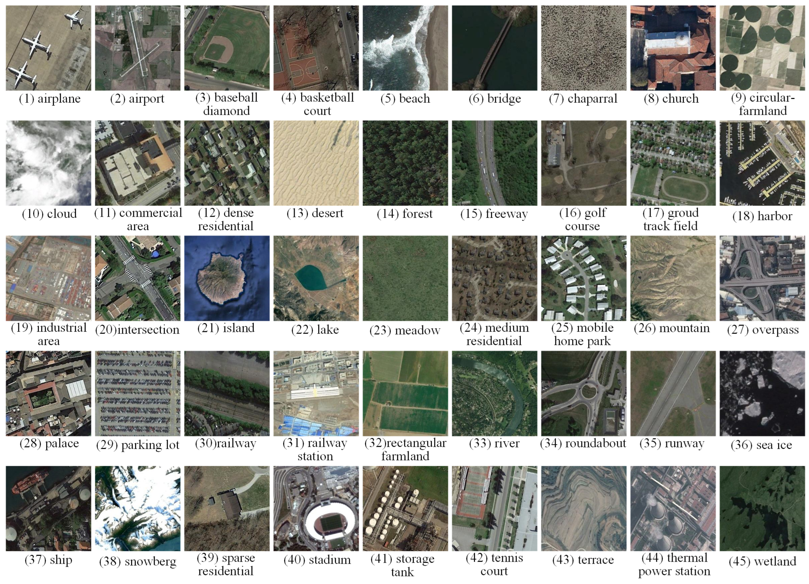
4.1.1. NWPU-RESISC45 Dataset

NWPU-RESISC45 is a large-scale remote sensing image scene classification dataset proposed by Northwestern Polytechnical University of China. Scene images in this dataset are selected from Google Earth by the professionals in remote sensing image processing, and 31,500 images are selected from more than 100 countries and regions of the world, which contain developing and developed countries and regions. Additionally, the maps of Google Earth are shown on a 3D globe, which is superimposed on satellite imagery, a geographic information system and aerial photography. This dataset is available in a variety of weathers, seasons, scales, imaging conditions, and illumination conditions. Except for some specific classes with low spatial resolution (such as island, lake, mountain), the pixel resolution of most scene classes is between 30 m and $0.2$ m, and the spectral bands of this dataset are red, green, and blue. The dataset contains 45 scene classes. As shown in Figure 6, the scene classes of this dataset include: airplane, airport, baseball diamond, basketball court, beach, bridge, chaparral, church, circular farmland, cloud, commercial area, dense residential, desert, forest, freeway, golf course, ground track field, harbor, industrial area, intersection, island, lake, meadow, medium residential, mobile home park, mountain, overpass, palace, parking lot, railway, railway station, rectangular farmland, river, roundabout, runway, sea ice, ship, snowberg, sparse residential, stadium, storage tank, tennis court, terrace, thermal power station, and wetland. Each scene class has 700 images with a size of $256\times 256$. In this paper’s experiment, this dataset is divided into 25, 10 and 10 classes for training, validation and testing, respectively.

4.1.2. UC Merced Dataset

The UC Merced dataset was released in 2010 and contains 21 scene classes. As shown in Figure 7, the scene classes of the UC Merced dataset include: agricultural, airplane, baseball diamond, beach, buildings, chaparral, dense residential, forest, freeway, golf course, harbor, intersection, medium density residential, mobile home park, overpass, parking lot, river, runway, sparse residential, storage tanks, and tennis courts. Each scene class consists of 100 land use images. The resolution of images in this dataset is $0.3$ m, the image size is $256\times 256$, and the image format is RGB. The UC Merced dataset is collected from the United States Geological Survey National Map, including the following regions of the United States: Birmingham, Boston, Buffalo, Columbus, Dallas, Harrisburg, Houston, Jacksonville, Las Vegas, Los Angeles, Miami, Napa, New York, Reno, San Diego, Santa Barbara, Seattle, Tampa, Tucson, and Ventura. So far, this dataset is still widely used in remote sensing image scene classification. In the experiment of this paper, this dataset is also divided into 10, 6 and 5 classes for training, validation and testing, respectively.

4.1.3. WHU-RS19 Dataset

WHU-RS19, published by Wuhan University in China, is a dataset for the scene classification of remote sensing images. It is collected from a series of satellite images extracted from Google Earth. The resolution of this dataset is 0.5 m, and the spectral bands of this dataset are red, green, and blue. As shown in Figure 8, this dataset contains 19 scene classes, namely: airport, beach, bridge, commercial area, desert, farmland, football field, forest, industrial area, meadow, mountain, park, parking lot, pond, port, railway station, residential area, river, and viaduct. Each scene class of this dataset contains at least 50 samples. The total number of samples in this dataset is 1005, and the image size is $600\times 600$. In the experiment of this paper, nine classes in the WHU-RS19 dataset are divided into a training dataset, five classes into a validation dataset, and five classes into a testing dataset.

The same split as DLA-MatchNet is used to divide the dataset $D_{total}$ into training dataset $D_{train}$, validation dataset $D_{val}$ and testing dataset $D_{test}$. They have their own label spaces and do not intersect each other, namely $D_{train}\cap D_{test}=⌀$, $D_{test}\cap D_{val}=⌀$, $D_{test}\cap D_{val}=⌀$, $D_{train}\cap D_{test}=⌀$, and $D_{train}\cup D_{val}\cup D_{test}=D_{total}$.

In addition, in a few-shot classification task, the divided datasets play different roles. $D_{train}$ is used to train the model, $D_{val}$ is used to adjust parameters and preliminarily evaluate the performance of the model, and $D_{test}$ is used to evaluate the generalization ability of the model to the unknown data.

4.2. Experimental Setting

In the experiment of this paper, the datasets used are NWPU-RESISC45, WHU-RS19 and UC Merced, and the average accuracy of top-1 is used to judge the classification results.

4.2.1. Experimental Software and Hardware Environment

The software and hardware environment used in the experiment are shown in

Table 1. The software and hardware environment used in the experiment.

Hardware Environment	CPU	Intel(R) Core(TM) i7-7800X CPU @ 3.50 GHz 32 GB
	GPU	NVIDIA Geforce RTX 2080Ti 11 GB
Software Environment	OS	Linux Ubuntu 18,04 LTS
	Programing Language	python 3.6
	Deep Learning Framework	Pytorch 1.4.0
	CUDA	Cuda 10.0

.

4.2.2. Experimental Design

The deep embedding module of our method in this paper selects ResNet18 after removing the fully connected layer and the last two convolutional blocks, as shown in the Figure 4. The input image is randomly cropped to $224\times 224$ and enhanced by a random horizontal flip, brightness enhancement, color enhancement, contrast enhancement, etc. The number of k-nearest neighbors searched in the metric module is set to 3.

All experiments are performed around the C-way K-shot classification task of the above datasets. This paper mainly selects two typical few-shot learning classification tasks: 5-way 1-shot and 5-way 5-shot. In order to achieve a fair comparison, the task has set parameters similar to those in the previous work of other scholars [33]. In the training process, the model is trained through episodic training. With random sampling in the support set, $300,000$ episodes are constructed. In each episode, each class not only contains K support images, but also, respectively, selects 15 and 10 query images from the class for the 1-shot and 5-shot tasks. That is, for a 5-way 1-shot task, an episode will include 5 support images and 75 query images. For a 5-way 5-shot task, there will be 25 support images and 50 query images in an episode. During the training process, the Adam [44] algorithm is used, and the initial learning rate is set to 0.0001, which decays for every 100,000 episodes. Overall, 600 episodes are constructed in the validation datasets for quick testing. After every 10,000 episodes are trained, an experiment is conducted on the verification dataset. The average value is the training result of the current network, and the model with the highest index is finally saved as the final model. The average accuracy value is taken as the training result, and the model with the highest accuracy is finally saved as the final model. During the testing process, 600 few-shot classification tasks are constructed by random sampling in the testing dataset, and the average accuracy of the top-1 is calculated. Repeat the process five times, take the average value of the five testing results as the final testing result, and the $95\%$ confidence intervals are given. Our model is trained in an end-to-end manner and does not require fine-tuning during the testing stage.

4.2.3. Evaluating Indicator

Because the testing of few-shot classification task requires random sampling of datasets in each round, there are differences in the distribution of samples in each round of the testing task. It is not reliable to use accuracy only. Therefore, the evaluating indicator used in this experiment is the top-1 accuracy rate, and it gives $95\%$ confidence intervals (CI). The classification accuracy is calculated as follows:

$$\begin{array}{cc}\hfill & acc=\frac{T_{nums}}{A_{nums}}\hfill \end{array}$$

(9)

where $T_{nums}$ represents the number of correctly classified samples, and $A_{nums}$ represents the number of all samples.

CI refers to the boundary of the estimation of the overall variable, which is used to quantify the uncertainty of the estimated value, so as to evaluate the reliability of the model. The mean value $mea{n}_{acc}$ of the accuracy rate and the overall standard deviation ${\delta }_{acc}$ of the accuracy rate can be obtained according to the multiple accuracy rates. Additionally, the $1-\alpha$ confidence interval of average overall accuracy rate can be calculated as follows:

$$\begin{array}{cc}\hfill & CI=\left(mea{n}_{acc}-Z_{\frac{\alpha }{2}}\times \frac{{\delta }_{acc}}{\sqrt{n}},mea{n}_{acc}+Z_{\frac{\alpha }{2}}\times \frac{{\delta }_{acc}}{\sqrt{n}}\right)\hfill \end{array}$$

(10)

where the Z value can be obtained by looking up the standard normal distribution table, n is the number of tests, and $\frac{{\delta }_{acc}}{\sqrt{n}}$ represents the standard error of the test sample.

4.3. Experimental Results

In this paper, the experiments are, respectively, conducted on NWPU-RESISC45, UC Merced and WHU-RS19 on 5-way 1-shot task and 5-way 5-shot task, and the effectiveness of our method for few-shot remote sensing image scene classification is verified by comparing with other few-shot classification methods.

The compared methods include MatchingNet [35], RelationNet [45], MAML [46], Meta-SGD [47], DLA-MatchNet [24] and DN4 [33]. Among them, MatchingNet, RelationNet, MAML, and Meta-SGD are four representative few-shot learning methods. Since our method is based on the DN4 framework, DN4 with the same embedding network as our method will be used for comparison. DLA-MatchNet is one of the most advanced networks for few-shot scene classification of remote sensing images. It is proposed based on the matching network, and uses the attention mechanism to deeply study the channel relationship and spatial relationship between features, in order to automatically discover the distinguishable regions. The experimental results of different methods on the three datasets are shown in

Table 2. Experimental results of different methods on the NWPU-RESISC45 dataset.

Method	5-Way 1-Shot	5-Way 5-Shot
MatchingNet	54.46% ± 0.77%	67.87% ± 0.59%
RelationNet	58.61% ± 0.83%	78.63% ± 0.52%
MAML	37.36% ± 0.69%	45.94% ± 0.68%
Meta-SGD	60.63% ± 0.90%	75.75% ± 0.65%
DLA-MatchNet	68.80% ± 0.70%	81.63% ± 0.46%
DN4	66.39% ± 0.86%	83.24% ± 0.87%
Our Method	70.75% ± 0.81%	86.79% ± 0.51%

,

Table 3. Experimental results of different methods on the UC Merced dataset.

Method	5-Way 1-Shot	5-Way 5-Shot
MatchingNet	46.16% ± 0.71%	66.73% ± 0.56%
RelationNet	48.89% ± 0.73%	64.10% ± 0.54%
MAML	43.65% ± 0.68%	58.43% ± 0.64%
Meta-SGD	50.52% ± 2.61%	60.82% ± 2.00%
DLA-MatchNet	53.76% ± 0.62%	63.01% ± 0.51%
DN4	57.25% ± 1.01	79.74% ± 0.78%
Our Method	65.49% ± 0.72%	85.73% ± 0.47%

and

Table 4. Experimental results of different methods on the WHU-RS19 dataset.

Method	5-Way 1-Shot	5-Way 5-Shot
MatchingNet	60.60% ± 0.68%	82.99% ± 0.40%
RelationNet	60.54% ± 0.71%	76.24% ± 0.34%
MAML	46.72% ± 0.55%	79.88% ± 0.41%
Meta-SGD	51.54% ± 2.31%	61.74% ± 2.02%
DLA-MatchNet	68.27% ± 1.83%	79.89% ± 0.33%
DN4	82.14% ± 0.80%	96.02% ± 0.33%
Our Method	85.05% ± 0.52%	96.94% ± 0.21%

, and the bold numbers in the table represent the best results.

As can be seen from the experimental results in Table 2, Table 3 and Table 4, no matter if it is a 5-way 1-shot or 5-way 5-shot task, the accuracy of our method is the highest on the three datasets, which indicates that our method has the best classification performance and can effectively improve the accuracy of few-shot remote sensing image scene classification.

4.4. Discussion

MAML and Meta-SGD are based on optimization strategies to solve few-shot learning problems. The parameters of the MAML [46] model are trained in an explicit manner, in order to ensure that a small quantity of gradient steps and few training data from a new task will yield excellent generalization results on that task. All the elements of an optimizer are learned by the Meta-SGD [47] model, including: initialization, learning rate, and update direction. In this way, Meta-SGD achieves a better performance in few-shot learning compared to other optimizer-based methods. MAMAL and Meta-SGD are the model-agnostic methods and applicable to any model trained through gradient descent. However, only relying on optimization strategies usually cannot obtain good few-shot remote sensing image classification results, which can also be proved by the contents of the experimental results section. MatchingNet [35] and RelationNet [45] are the representative models based on deep learning architecture design and metric learning. Matching-Net learns a non-parametric network based on metric learning, avoiding the consumption of fine-tuning to adjust to different classes. RelationNet designs a deep architecture, which consists of a deep embedding module and deep distance metric module. Because the deep architectures of MatchingNet and RelationNet are specially designed for few-shot learning, they obtain better few-shot remote sensing image scene classification results than MAMAL and Meta-SGD. Additionally, it can also be proven that specialized deep architecture design is usually more effective than just an optimization strategy. The architecture of DLA-MatchNet [24] is similar to that of MatchingNet and RelationNet, but DLA-MatchNet designs a proper discriminative representations method and special metric method for remote sensing scene images. Therefore, the few-shot remote sensing image scene classification results of DLA-MatchNet are better than that of MatchingNet and RelationNet. The local descriptor based on an image-to-class measure method is utilized in DN4 [33], which is executed through a k-nearest neighbor search method on the local descriptors of deep feature maps. Because DN4 directly constructs a measure bridge between image and class, DN4 achieves better few-shot remote sensing image scene classification results than that of the above-mentioned compared methods. Compared with DN4, our method introduces the non-local attention mechanism on the local descriptor. The attention map obtained in the attention-based deep embedding module is used in our method to weighted sum the similarity of descriptors. Through this manner, the local descriptor representing the scene class will have a higher impact on the final classification result due to its higher weight, while the local descriptor in the interference region has a lower weight, thus reducing the impact of the interference. Therefore, our method obtains better few-shot remote sensing image scene classification results than that of the compared methods.

In summary, our method can produce such excellent classification results mainly due to two factors. Firstly, to solve the problem of sparse image-level features in few-shot conditions, a local descriptor to represent the features is used in our method, making full use of the local feature information of images, and avoiding the problem that it is difficult to effectively represent classes in few-shot conditions due to too few image-level features. Secondly, the class-related attention module proposed in this paper can obtain the class-related attention map, thus increasing the weight of the class-related local descriptors in the metric process, highlighting representative local descriptors, and finally reducing the interference of noise.

Next, we discuss the influence of hyperparameter k. In the metric module, it is necessary to find k nearest neighbors for each local descriptor of the query image in a support class, and then measure the image-to-class similarity between the query image and that class. Therefore, how to select the appropriate hyperparameter k is critical. To this end, this experiment executes the 5-way 5-shot task with a different k value on the NWPU-RESISC45 dataset. The classification results are shown in

Table 5. Classification results of our method with different k values on the NWPU-RESISC45 dataset.

Method	$\mathit{k}=1$	$\mathit{k}=2$	$\mathit{k}=3$	$\mathit{k}=4$
Our Method	86.65%	86.69%	86.79%	86.88%

, where the bold numbers indicate the best results, and it can be seen that the k value has little effect on the classification performance. Furthermore, the greater the value of K, the greater the computational burden. Thus, our method selects the same k value as in the DN4 network, namely setting k = 3.

In order to select a suitable embedding network, we study the performance of different networks as deep embedding networks. In the compared experiment, four shallow networks, namely Conv-64F [34], VGG16 [25], ResNet18 [26] and ResNet50 [26], are used. Conv-64F is a commonly used embedding network in few-shot learning methods, and it is also used as the backbone network in the DN4 model. Figure 9 shows the results of our method using different embedding networks on the NWPU-RESISC45 dataset, and it is easy to see from the histogram that ResNet18 has the highest accuracy on both 1-shot and 5-shot tasks. The accuracies of the Conv-64F and VGG16 networks are lower, while ResNet50 is over-fitting. Therefore, ResNet18 is selected as the embedding module of our method.

In order to more intuitively display the function of the scene-related attention module of our method, the attention feature map obtained by this module is visualized, as shown in Figure 10, which shows part of the samples in the NWPU-RESISC45 dataset. From top to bottom is the original image, the class-related attention feature map of the image, and the fusion image of the two. In roundabout and highway scenes, the attention module can correctly identify the part of the road, unaffected by backgrounds such as trees. In the basketball court, track and field and ship scenes, the network also focuses on the basketball court, runway, ship and other related object areas. It is proved again that our method can avoid the negative impact of complex backgrounds and has good classification performance in remote sensing image scene classification tasks.

5. Conclusions

In this paper, a novel method, namely DN4AM, is proposed to solve the problem of complex backgrounds in few-shot remote sensing image scene classification. In order to solve the problem of few-shot learning, our method introduces episodic training. For solving the problem of sparse image-level features in few-shot conditions, deep local descriptors are used for feature representation to make full use of local feature information of an image. In order to suppress the influence of scene class-independent regions in the image, the attention mechanism is introduced to obtain scene class-related attention maps, which distinguish the deep local descriptors into a scene-related part and scene-unrelated part. The similarity between the local descriptor of the query image and the class is calculated based on the metric module, and the weighted summations are carried out by using the attention map. Finally, the summations are taken as the final prediction probability value. Experiments show that the our method can avoid the interference of a complex background in the scene image, which is more suitable for the few-shot scene classification of remote sensing images. As to few-shot remote sensing image scene classification, image-to-class measurement and attention mechanism are very helpful, and a specialized deep architecture design is usually more effective than just an optimization strategy. Furthermore, the focus of this paper is to reasonably introduce the attention mechanism for the local descriptor-based image-to-class measurement. In the future, we will give a further study on the attention mechanism for our work, including Coordinate Attention [48], CBAM [49], ECA [50], and SimAM [51].

References

- Bai, T.; Wang, H.; Wen, B. Targeted Universal Adversarial Examples for Remote Sensing. Remote Sens. 2022, 14, 5833. [Google Scholar] [CrossRef]
- Muhammad, U.; Hoque, M.; Wang, W.; Oussalah, M. Patch-Based Discriminative Learning for Remote Sensing Scene Classification. Remote Sens. 2022, 14, 5913. [Google Scholar] [CrossRef]
- Chen, X.; Zhu, G.; Liu, M. Remote Sensing Image Scene Classification with Self-Supervised Learning Based on Partially Unlabeled Datasets. Remote Sens. 2022, 14, 5838. [Google Scholar] [CrossRef]
- Jiang, N.; Shi, H.; Geng, J. Multi-Scale Graph-Based Feature Fusion for Few-Shot Remote Sensing Image Scene Classification. Remote Sens. 2022, 14, 5550. [Google Scholar] [CrossRef]
- Xing, S.; Xing, J.; Ju, J.; Hou, Q.; Ding, X. Collaborative Consistent Knowledge Distillation Framework for Remote Sensing Image Scene Classification Network. Remote Sens. 2022, 14, 5186. [Google Scholar] [CrossRef]
- Xiong, Y.; Xu, K.; Dou, Y.; Zhao, Y.; Gao, Z. WRMatch: Improving FixMatch with Weighted Nuclear-Norm Regularization for Few-Shot Remote Sensing Scene Classification. IEEE Trans. Geosci. Remote Sens. 2022, 60, 1–14. [Google Scholar] [CrossRef]
- Wang, X.; Xu, H.; Yuan, L.; Dai, W.; Wen, X. A remote-sensing scene-image classification method based on deep multiple-instance learning with a residual dense attention ConvNet. Remote Sens. 2022, 14, 5095. [Google Scholar] [CrossRef]
- Gao, Y.; Sun, X.; Liu, C. A General Self-Supervised Framework for Remote Sensing Image Classification. Remote Sens. 2022, 14, 4824. [Google Scholar] [CrossRef]
- Zhao, Y.; Liu, J.; Yang, J.; Wu, Z. Remote Sensing Image Scene Classification via Self-Supervised Learning and Knowledge Distillation. Remote Sens. 2022, 14, 4813. [Google Scholar] [CrossRef]
- Cheng, G.; Guo, L.; Zhao, T.; Han, J.; Li, H.; Fang, J. Automatic landslide detection from remote-sensing imagery using a scene classification method based on BoVW and pLSA. Int. J. Remote Sens. 2013, 34, 45–59. [Google Scholar] [CrossRef]
- Lv, Z.; Shi, W.; Zhang, X.; Benediktsson, J. Landslide inventory mapping from bitemporal high-resolution remote sensing images using change detection and multiscale segmentation. IEEE J. Sel. Top. Appl. Earth Observ. 2018, 11, 1520–1532. [Google Scholar] [CrossRef]
- Longbotham, N.; Chaapel, C.; Bleiler, L.; Padwick, C.; Emery, W.; Pacifici, F. Very high resolution multiangle urban classification analysis. IEEE Trans. Geosci. Remote Sens. 2011, 50, 1155–1170. [Google Scholar] [CrossRef]
- Tayyebi, A.; Pijanowski, B.; Tayyebi, A. An urban growth boundary model using neural networks, GIS and radial parameterization: An application to Tehran, Iran. Landscape Urban Plan. 2011, 100, 35–44. [Google Scholar] [CrossRef]
- Huang, X.; Wen, D.; Li, J.; Qin, R. Multi-level monitoring of subtle urban changes for the megacities of China using high-resolution multi-view satellite imagery. Remote Sens. Environ. 2017, 196, 56–75. [Google Scholar] [CrossRef]
- Zhang, T.; Huang, X. Monitoring of urban impervious surfaces using time series of high-resolution remote sensing images in rapidly urbanized areas: A case study of Shenzhen. IEEE J. Sel. Top. Appl. Earth Observ. 2018, 11, 2692–2708. [Google Scholar] [CrossRef]
- Li, X.; Shao, G. Object-based urban vegetation mapping with high-resolution aerial photography as a single data source. Int. J. Remote Sens. 2013, 34, 771–789. [Google Scholar] [CrossRef]
- Rußwurm, M.; Körner, M. Multi-temporal land cover classification with sequential recurrent encoders. ISPRS Int. J. Geo-Inf. 2018, 7, 129. [Google Scholar] [CrossRef]
- Lowe, D. Distinctive image features from scale-invariant keypoints. Int. J. Comput. Vis. 2004, 60, 91–110. [Google Scholar] [CrossRef]
- Swain, M.; Ballard, D. Color indexing. Int. J. Comput. Vis. 1991, 7, 11–32. [Google Scholar] [CrossRef]
- Dalal, N.; Triggs, B. Histograms of oriented gradients for human detection. In Proceedings of the IEEE Conference on Computer Vision and Pattern Recognition, San Diego, CA, USA, 20–26 June 2005; pp. 886–893. [Google Scholar]
- Oliva, A.; Torralba, A. Modeling the shape of the scene: A holistic representation of the spatial envelope. Int. J. Comput. Vis. 2001, 42, 145–175. [Google Scholar] [CrossRef]
- Hinton, G.; Salakhutdinov, R. Reducing the dimensionality of data with neural networks. Science 2006, 313, 504–507. [Google Scholar] [CrossRef] [PubMed]
- Olshausen, B.; Field, D. Sparse coding with an over-complete basis set: A strategy employed by V1? Vis. Res. 1997, 37, 3311–3325. [Google Scholar] [CrossRef]
- Li, L.; Han, J.; Yao, X.; Cheng, G.; Guo, L. DLA-MatchNet for few-shot remote sensing image scene classification. IEEE Trans. Geosci. Remote Sens. 2020, 59, 7844–7853. [Google Scholar] [CrossRef]
- Simonyan, K.; Zisserman, A. Very deep convolutional networks for large-scale image recognition. arXiv 2014, arXiv:1409.1556v6. [Google Scholar]
- He, K.; Zhang, X.; Ren, S.; Sun, J. Deep residual learning for image recognition. In Proceedings of the IEEE Conference on Computer Vision and Pattern Recognition (CVPR), Las Vegas, CA, USA, 27–30 June 2016; pp. 770–778. [Google Scholar]
- Krizhevsky, A.; Sutskever, I.; Hinton, G.E. Imagenet classification with deep convolutional neural networks. Adv. Neural Inf. Process. Syst. 2012, 25, 5–9. [Google Scholar] [CrossRef]
- Szegedy, C.; Liu, W.; Jia, Y.; Sermanet, P.; Reed, S.; Anguelov, D.; Erhan, D.; Vanhoucke, V.; Rabinovich, A. Going deeper with convolutions. In Proceedings of the IEEE Conference on Computer Vision and Pattern Recognition, Boston, MA, USA, 7–12 June 2015; pp. 1–9. [Google Scholar]
- Gui, R.; Xu, X.; Yang, R.; Wang, L.; Pu, F. Statistical scattering component-based subspace alignment for unsupervised cross-domain PolSAR image classification. IEEE Trans. Geosci. Remote Sens. 2020, 59, 5449–5463. [Google Scholar] [CrossRef]
- Zhou, H.; Du, X.; Li, S. Self-Supervision and Self-Distillation with Multilayer Feature Contrast for Supervision Collapse in Few-Shot Remote Sensing Scene Classification. Remote Sens. 2022, 14, 3111. [Google Scholar] [CrossRef]
- Huang, W.; Yuan, Z.; Yang, A.; Tang, C.; Luo, X. TAE-Net: Task-Adaptive Embedding Network for Few-Shot Remote Sensing Scene Classification. Remote Sens. 2022, 14, 111. [Google Scholar] [CrossRef]
- Kim, J.; Chi, M. AFFNet: Self-Attention-Based Feature Fusion Network for Remote Sensing Few-Shot Scene Classification. Remote Sens. 2021, 13, 2532. [Google Scholar] [CrossRef]
- Li, W.; Wang, L.; Xu, J.; Huo, J.; Gao, Y.; Luo, J. Revisiting Local Descriptor Based Image-To-Class Measure for Few-Shot Learning. arXiv 2019, arXiv:1903.12290v2. [Google Scholar]
- Boiman, O.; Shechtman, E.; Irani, M. In defense of nearest-neighbor based image classification. In Proceedings of the IEEE Conference on Computer Vision and Pattern Recognition (CVPR), Anchorage, AK, USA, 23–28 June 2008; pp. 1–8. [Google Scholar]
- Vinyals, O.; Blundell, C.; Lillicrap, T.; Wierstra, D. Matching networks for one shot learning. In Proceedings of the Advances in Neural Information Processing Systems, Barcelona, Spain, 5–10 December 2016; pp. 3630–3638. [Google Scholar]
- Hu, J.; Shen, L.; Sun, G. Squeeze-and-excitation networks. In Proceedings of the IEEE Conference on Computer Vision and Pattern Recognition (CVPR), Salt Lake City, UT, USA, 18–22 June 2018; pp. 7132–7141. [Google Scholar]
- Fukunaga, K.; Narendra, P. A branch and bound algorithm for computing k-nearest neighbors. IEEE Trans. Comput. 1975, 100, 750–753. [Google Scholar] [CrossRef]
- Wei, Y.; Yen, C.; Zsolt, K.; Yu, C.; Frank, W.; Jia, B. A closer look at few-shot classification. In Proceedings of the International Conference on Learning Representations (ICLR), New Orleans, LA, USA, 6–9 May 2019; pp. 1–17. [Google Scholar]
- Lin, M.; Chen, Q.; Yan, S. Network In Network. arXiv 2013, arXiv:1312.4400. [Google Scholar]
- Wang, X.; Girshick, R.; Gupta, A.; He, K. Non-local neural networks. In Proceedings of the IEEE Conference on Computer Vision and Pattern Recognition (CVPR), Salt Lake City, UT, USA, 18–22 June 2018; pp. 7794–7803. [Google Scholar]
- Cheng, G.; Han, J.; Lu, X. Remote sensing image scene classification: Benchmark and state of the art. Proc. IEEE 2017, 105, 1865–1883. [Google Scholar] [CrossRef]
- Yang, Y.; Newsam, S. Bag-of-visual-words and spatial extensions for land-use classification. In Proceedings of the 18th SIGSPATIAL International Conference on Advances in Geographic Information Systems, San Jose, CA, USA, 2–5 November 2010; pp. 270–279. [Google Scholar]
- Sheng, G.; Yang, W.; Xu, T.; Sun, H. High-resolution satellite scene classification using a sparse coding based multiple feature combination. Int. J. Remote Sens. 2012, 33, 2395–2412. [Google Scholar] [CrossRef]
- Kingma, D.; Ba, J. Adam: A Method for Stochastic Optimization. In Proceedings of the International Conference on Learning Representations (ICLR), San Diego, CA, USA, 7–9 May 2015. [Google Scholar]
- Sung, F.; Yang, Y.; Zhang, L.; Xiang, T.; Torr, P.; Hospedales, T. Learning to compare: Relation network for few-shot learning. In Proceedings of the IEEE Conference on Computer Vision and Pattern Recognition (CVPR), Salt Lake City, UT, USA, 18–22 June 2018; pp. 1199–1208. [Google Scholar]
- Finn, C.; Abbeel, P.; Levine, S. Model-agnostic meta-learning for fast adaptation of deep networks. In Proceedings of the International Conference on Machine Learning (ICML), Sydney, Australia, 6–11 August 2017; pp. 1126–1135. [Google Scholar]
- Li, Z.; Zhou, F.; Chen, F.; Li, H. Meta-sgd: Learning to learn quickly for few-shot learning. arXiv 2017, arXiv:1707.09835v2. [Google Scholar]
- Hou, Q.; Zhou, D.; Feng, J. Coordinate attention for efficient mobile network design. In Proceedings of the IEEE/CVF Conference on Computer Vision and Pattern Recognition (CVPR), Online, 19–25 June 2021; pp. 13713–13722. [Google Scholar]
- Woo, S.; Park, J.; Lee, J.; Kweon, I. Cbam: Convolutional block attention module. In Proceedings of the European Conference on Computer Vision (ECCV), Munich, Germany, 8–14 September 2018; pp. 3–19. [Google Scholar]
- Wang, Q.; Wu, B.; Zhu, P.; Li, P.; Zuo, W.; Hu, Q. ECA-Net: Efficient Channel Attention for Deep Convolutional Neural Networks. arXiv 2019, arXiv:1910.03151. [Google Scholar]
- Yang, L.; Zhang, R.; Li, L.; Xie, X. Simam: A simple, parameter-free attention module for convolutional neural networks. In Proceedings of the International Conference on Machine Learning (ICML), Online, 18–24 July 2021; pp. 11863–11874. [Google Scholar]