Multi-Swin Mask Transformer for Instance Segmentation of Agricultural Field Extraction

Abstract

With the rapid development of digital intelligent agriculture, the accurate extraction of field information from remote sensing imagery to guide agricultural planning has become an important issue. In order to better extract fields, we analyze the scale characteristics of agricultural fields and incorporate the multi-scale idea into a Transformer. We subsequently propose an improved deep learning method named the Multi-Swin Mask Transformer (MSMTransformer), which is based on Mask2Former (an end-to-end instance segmentation framework). In order to prove the capability and effectiveness of our method, the iFLYTEK Challenge 2021 Cultivated Land Extraction competition dataset is used and the results are compared with Mask R-CNN, HTC, Mask2Former, etc. The experimental results show that the network has excellent performance, achieving a bbox_AP50 score of 0.749 and a segm_AP50 score of 0.758. Through comparative experiments, it is shown that the MSMTransformer network achieves the optimal values in all the COCO segmentation indexes, and can effectively alleviate the overlapping problem caused by the end-to-end instance segmentation network in dense scenes.

1. Introduction

The spatial distribution of agricultural fields refers to the location and extent of the fields, and is needed to establish the area of land utilized for agricultural yield prediction, resource allocation, and economic planning [1,2,3,4]. In addition to its ecological and economic value, it is also indispensable in management and decision-making. The digital management of farmland can help the whole agricultural industry and related enterprises to monitor and manage crop production analysis through networks [5]. Accurate field-boundary digital recording is very important for digital agriculture. However, this process is still mainly a manual operation which relies heavily on manual work. This is time-consuming work, and will incur errors due to human factors [6,7]. Using remote sensing technology to realize the automatic extraction of fields is very important in the development of intelligent agriculture, ecology, and economy.

There are many methods to extract fields based on remote sensing images, but most of them still do not have good generalization ability. These methods can be broadly divided into three categories:

(1)

Edge-based methods. These methods mainly use filters (such as Sobel, Canny [8], etc.) to extract the edges in the image, and use the extracted edges as the field boundary [9]. In order to obtain more accurate edges, some methods are assisted by NDVI [10]. There are many problems in this method. Firstly, the edge detection operator is susceptible to high-frequency noise. Even after Gaussian smoothing, the image will still have noise so that clean edge extraction cannot be achieved. The stronger the texture of the field, the greater the interference. Secondly, the results of edge detection are not connected, resulting in an inability to obtain closed fields. Finally, this method cannot be used independently. Usually, a remote sensing image contains more extra information than fields. Therefore, the field/non-field classification is required before edge extraction, resulting in a very cumbersome process.

(2)

Region-based methods such as selective search [11], the watershed algorithm [12], region growing, etc. There are many region based algorithms, which are usually integrated into the OpenCV tool library or implemented by software such as eCognition [13]. These methods group the adjacent pixels by feature (color, texture, etc.), and then, divide the image into several groups by continuously merging the surrounding pixels into one group and setting the super parameter as the loop termination condition. Watkins et al. realized the extraction of a farmland boundary through the watershed segmentation algorithm and some post-processing [14]. The defect of this method is also obvious. The region-based algorithm relies on the relevant segmentation algorithm, which tends to over-segment fields with high internal variability and under-segment small adjacent fields [6].

(3)

Machine learning-based methods. With the development of machine learning, especially deep learning, traditional image processing algorithms are being replaced. There are many machine learning methods, such as random forest, support vector machine, and the more popular convolutional neural network model [15,16,17]. Convolutional neural networks have been proven to be very effective in the field of computer vision, and have excellent performance in semantic segmentation, object detection, instance segmentation, and other tasks. For example, Wang et al. succeeded in the automatic detection of pothole distress and pavement cracks using an improved convolutional neural network [18,19]. Especially in recent years, with the development of the Transformer, deep learning has been pushed to a new height [20]. A Transformer is used for automatic pavement image classification [21], remote sensing imagery semantic segmentation [22], hyperspectral image classification [23], etc. In the task of field extraction, the deep learning method is gradually used. For example, the method of semantic segmentation is used to extract the farmland area and the ridge area, respectively, and then the results are combined [6]. Zhao et al. used the Hybrid Task Cascade (HTC) network to segment remote sensing images, and combined this with an overlapping and tiling strategy for post-processing [24,25]. Instance segmentation is very suitable for the intensive segmentation task of field extraction, because there is hardly any post-processing of the results. Thus, the focus of this study is on instance segmentation.

Instance segmentation is a higher-level task combining object detection and semantic segmentation. It not only needs to distinguish different instances, but also needs to be marked with a mask. The development of instance segmentation started with Mask R-CNN [16]. After that, improved versions of Cascade R-CNN and HTC appeared [26]. This kind of instance segmentation model can be considered an enhanced version of the target detection model. A semantic segmentation detector is added at the tail, and still includes processes such as anchor and non-maximum suppression (NMS). With the emergence of DETR (end-to-end object detection with transformers) [27], the end-to-end detection framework has become popular. The characteristics of this kind of detector are that it cancels the process of anchor and NMS and treats target detection as a matching problem, and the output of the network model is the final output. Mask2Former follows this idea, implements an end-to-end instance segmentation model, and sets a new state-of-the-art for panoptic segmentation (57.8 PQ on COCO), instance segmentation (50.1 AP on COCO), and semantic segmentation (57.7 mIoU on ADE20K) [17].

This paper introduces a new model based on Mask2Former, which creatively integrates a multi-scale shift window into the model, inspired by the Inception structure (proposed by GoogLeNet) [28], and discusses the impact of multi-scale shift-window parallel connection on the model. Our specific contributions are as follows:

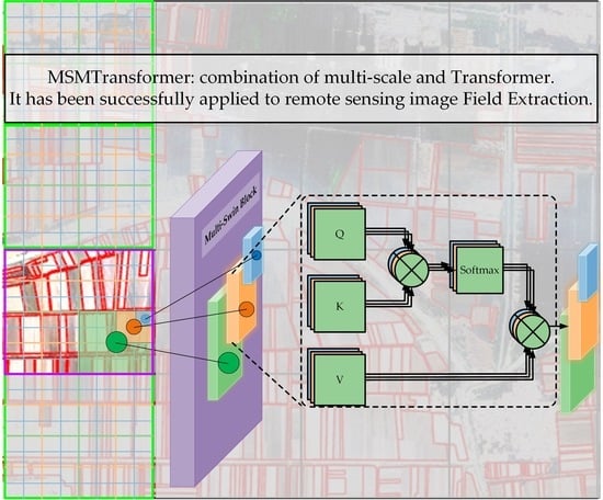
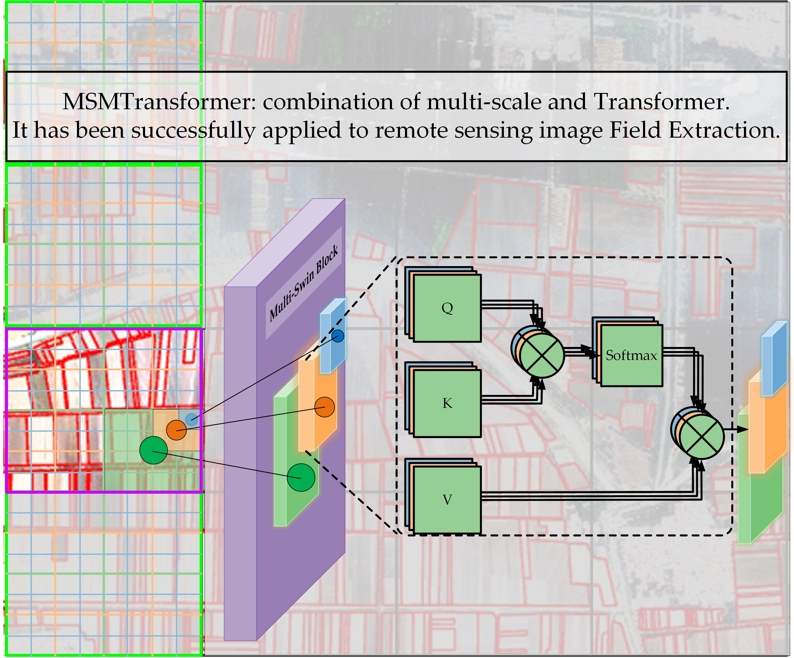
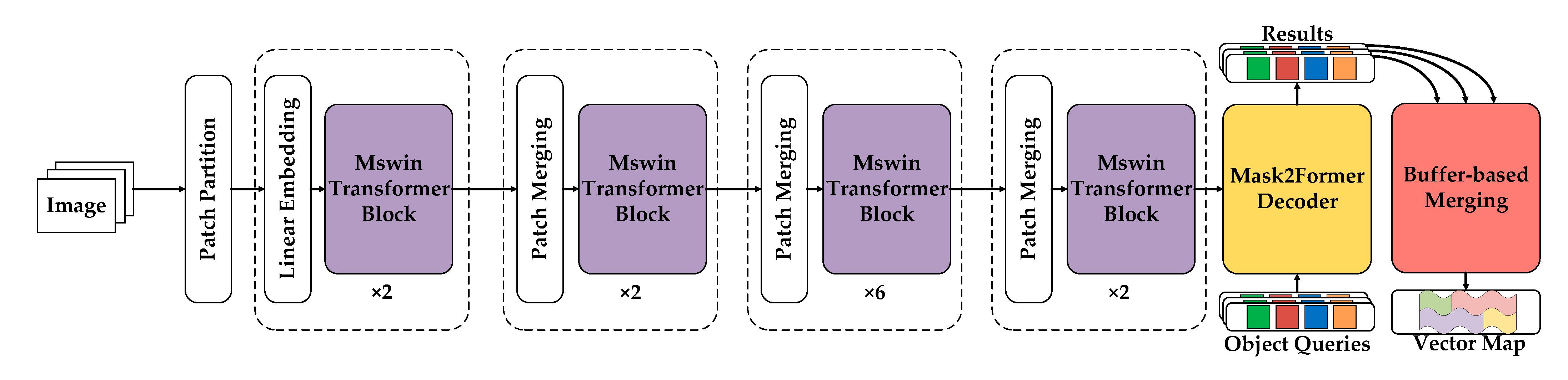
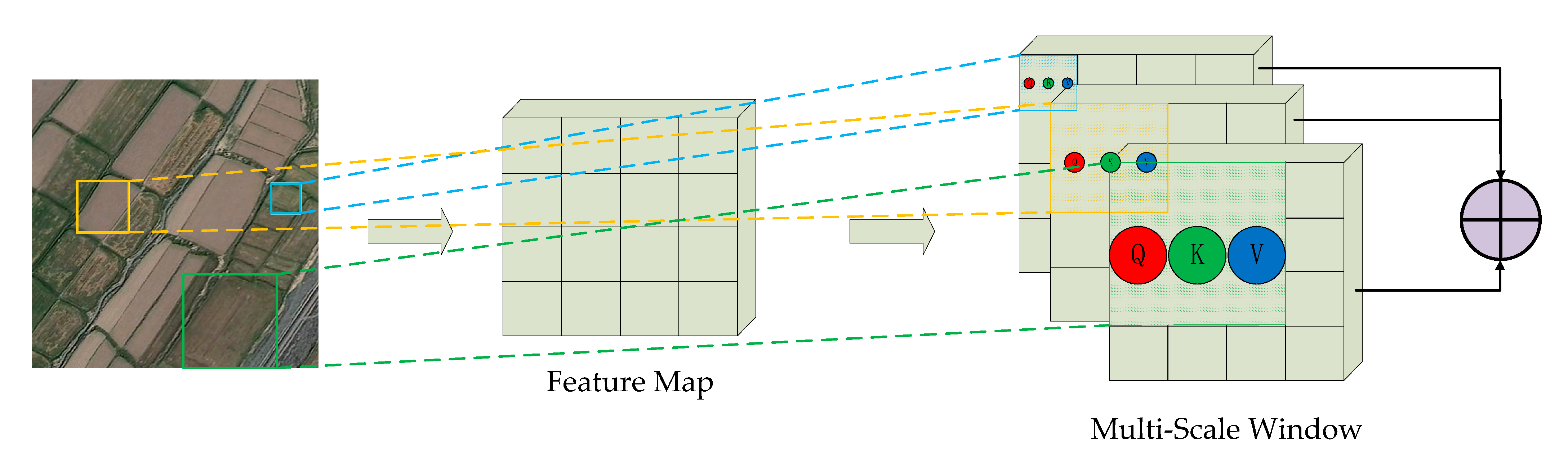
• The MSMTransformer network is proposed, which proves that the multi-scale shift window can effectively extract information in the process of self-attention, thereby improving the accuracy of instance segmentation. Additionally, we achieve a new state-of-the-art for instance segmentation using the iFLYTEK dataset [24].
• A process for integrating all felids at each image patch into one shape file is proposed for post-processing to avoid incomplete or overlapping results due to cropping.

2. Materials and Methods

We propose a Multi-Swin Mask Transformer network to detect agricultural fields from Jilin-1 imagery (Figure 1), which is a high-resolution dataset for field extraction from the competition held by iFLYTEK (Section 2.1). In order to better extract fields, we first reviewed the development of the Transformer in the image field and analyzed its shortcomings; subsequently, the MSMTransformer network is proposed for effectively extracting fields of different sizes and improving the accuracy of field extraction (Section 2.2). The details of the network and the structure of the Multi-Swin block are illustrated in Section 2.3.

2.1. Jilin-1 Image Dataset

Jilin-1 satellite constellation is the core project under construction by Changguang Satellite Technology Co., Ltd. in Changchun City, Jilin Province, China, and is an important optical remote sensing satellite constellation in China. To date, the total coverage area has reached 133 million square kilometers, which has been provided to users in the forestry, grassland, shipping, ocean, resource, and environmental industries, among others. The Jilin-1 image dataset from the 2021 iFLYTEK Challenge Cultivated Land Extraction was used in the form of high-resolution remote sensing images. Each image has four bands: blue, green, red, and near-infrared. The spatial resolution of the Jilin-1 multispectral images is 0.75–1.1 M [24]. This dataset provides 16 original images in Tiff format and their corresponding labels in shape-file format. Figure 1a shows an example of an original image and its corresponding labels in red.

In order to adapt to the input of the deep learning networks, at the data preprocessing stage, we cut 16 original images and processed them into COCO format [29]. The image size after processing was 512 × 512, and only the RGB channels were kept. Figure 1b shows examples of the processed images with a size of 512 × 512. The preprocessed images were divided into the training set and the validation set according to a 5:1 ratio, and the numbers of the processed images for the training set and validation set were 2950:601, respectively.

2.2. Transformer Reviewing

The Vision Transformer introduces the Transformer to the computer vision task for the first time [30]. In order to change an image into sequence data, VIT divides the image into 16 × 16 tokens and subsequently creates an Embedding layer and a Transformer Encoding layer. However, the number of tokens for a large-sized image is so large that the calculation of self-attention is too large.

In order to reduce the calculation amount for self-attention, the Swin Transformer puts forward the idea of a window, and only performs the self-attention operation inside the window [31]. At the same time, in the convolutional neural network [32], the convolutional operation is usually performed on the N × N pixels around the image pixel. This process can be considered the a priori addition of knowledge; the correlation between a pixel and its surrounding pixels should be the highest. The addition of the window by Swin Transformer not only reduces the amount of calculation, but also conforms to the idea of the CNN.

However, the fixed size of the window added by the Swin Transformer has limitations, and results in limited receptive fields [33]; consequently, it cannot adapt well to objects with different scales during feature extraction. Agricultural field extraction is a typical case with multiple scales; thus, the Jinlin-1 dataset is analyzed and is subsequently divided into three categories: small is no larger than 32 × 32 = 1024 pixels, medium is between 1024 and 9216 pixels, and large is no less than 96 × 96 = 9216 pixels. As shown in Figure 2, the numbers of fields with different scales in the training set and validation set are shown, and the proportion of the three scales is about 1:3:2. These statistics accurately describe the distribution of scales in the dataset. Consequently, we propose a multi-scale shift-window parallel mechanism to try to extract agricultural fields more accurately.

The multi-scale shift-window parallel mechanism used to integrate the information with different scales is employed as the backbone network to extract the fields. The detection head is still consistent with the Mask2Former. The overall architecture of the MSMTransformer is shown in Figure 3.

The Multi-Swin Transformer block is a module based on the attention mechanism. Compared with convolution, it has a larger receptive field and richer multi-scale sensors. After analyzing the incompleteness and overlap of the Swin Transformer in the field recognition process, we propose a multi-level window parallel structure, and its detailed model structure is shown in Figure 4.

2.3. Details of the Multi-Swin Block

We propose a parallel multi-scale shift window block to better extract contextual multi-scale information. Our block is embedded into the Swin Transformer Block [31]. Technically, given the input feature map $X^{\mathrm{L}-1}$, it will be normalized through the LayerNorm (LN) layer. Then, the normalized feature map is passed through our proposed MW-MSA module to obtain $X^{\mathrm{L}}$.

$$X^L=X^{L-1} +\mathit{MW-MSA}\left(\mathit{LN}\right(X^{L-1}\left)\right)$$

(1)

The module of MW-MSA is based on W-MSA [31], and W-MSA makes improvements on the basis of multi-head attention [34], so that the scope of the self-attention operation is limited to one rule window after another. We add a superscript to it to describe windows of different sizes.

$$Y^L=W\_MS{A}^{\alpha }(Y^{L-1})+W\_MS{A}^{\beta }(Y^{L-1})+W\_MS{A}^{\gamma }\left(Y^{L-1}\right)$$

(2)

where $Y^{L-1}$ denotes the result obtained after the feature map $X^{L-1}$ passes through the LN layer, and $Y^L$ denotes the result through MW-MSA.

Regarding the SMW-MSA module, we conducted parallel connection based on its shift window. Here, only the window position is changed, and the rest remains unchanged. More details can be obtained from the Transformer [34].

Figure 5 describes our design in detail. The red area represents windows of different sizes. The picture is divided into non-overlapping areas, and multi-head attention operations are performed independently within each window [31]. The windows of different sizes are connected in parallel, and a characteristic map of multiple receptive fields is subsequently fused. Finally, a residual connection is made with $X^{L-1}$.

2.4. Details of Parameter Settings

This section will introduce the detailed parameter settings of the MSMTransformer. It first splits an input image into non-overlapping patches using a patch splitting module, such as the Vision Transformer [30]. The patch size is set to 4 × 4, and then, the dimensions are transformed through the Linear Embedding layer. These two transformations are implemented via a convolution operation, where the convolution kernel size is 4 × 4, the stride is 4, and the output dimension is 96. Next is the stack of Multi-Swin Transformer Block and Patch Merging. Patch Merging is a 2× down-sampling operation [31] which is implemented via recombination splicing and a linear layer. The Mask2Form decoder is consistent with the baseline.

Figure 6 shows the parameters of important structures in the model. For the convolution operation, the four groups of numbers in the third column represent the input dimensions, convolution kernel size, stride, and output dimensions, respectively. For the Multi-Swin Transformer Block, it shows the size settings of parallel windows, the dimensions of the “Token”, and the number of heads in the multi-head self-attention. For the linear layer, the input and output dimensions are displayed, respectively. At last, for the decoder, it shows the number of input and output “object queries”.

3. Results

We conducted experiments on the iFLYTEK Challenge 2021 Cultivated Land Extraction competition data set, using the Mask R-CNN, HTC (the champion of the competition in 2021) [24], Mask2Former (our baseline), and the MSMTransformer network.

Mask R-CNN [16] was a new instance segmentation model based on Faster R-CNN. it was the best model at that time and outperformed all existing, single-model entries on every task. Mask R-CNN is representative of a two-stage detection method, and many works use it as a comparison model [35]. Later, there were many improvements to Mask R-CNN, such as HTC, which mixed the idea of hybrid cascading to explore more context information. By adding an additional semantic segmentation branch and merging it with box and mask branches, the accuracy was greatly improved. Mask2Former was the best instance segmentation network on the COCO dataset when it was proposed. It performs best when the Swin Transformer is selected as its backbone network.

The results show the effectiveness of the Multi-Swin block; in particular, the proposed network alleviates the overlapping problem, which is a common problem in end-to-end instance segmentation networks. The details are as follows.

3.1. Quantitative Comparison

In order to better prove the effectiveness of the multi-scale shift window, in the experiment of the Mask2Former model (baseline), we first carried out experiments on different single window sizes, and then, used Swin-S with more parameters as the backbone. The experiments show that changing the window size or overlapping more Swin blocks cannot bring better results, and can even cause overfitting.

The performance of all the models on this dataset is shown in

Table 1. Instance segmentation results on the validation set. Our model is superior to the baseline for most of the indicators.

Model	AP (bbox)	AP50 (bbox)	AP75 (bbox)	AP (segm)	AP50 (segm)	AP75 (segm)	Param (M)
Mask R-CNN	0.433	0.682	0.460	0.401	0.653	0.429	44.12
HTC *	0.529	0.753	0.583	0.496	0.734	0.542	139.79
Mask2Former (Swin-T-7)	0.522	0.742	0.562	0.523	0.754	0.566	47.40
Mask2Former (Swin-T-12)	0.518	0.740	0.559	0.513	0.745	0.555	47.45
Mask2Former (Swin-S-7)	0.515	0.743	0.557	0.517	0.747	0.564	68.72
Ours (5-7-11)	0.535	0.749	0.583	0.527	0.758	0.575	64.76

HTC * means the HTC network joins the DCN and FPN modules. This state-of-the-art model is used on the dataset from the competition [24]. Swin-T-7 means that the backbone network is Swin-T, and a single window with a size of 7 is set. The hyperparameters of the three parallel windows are set to 5, 7, and 11, respectively, in our model.

, and the MSMTransformer reaches new state-of-the-art accuracy on the experimental dataset.

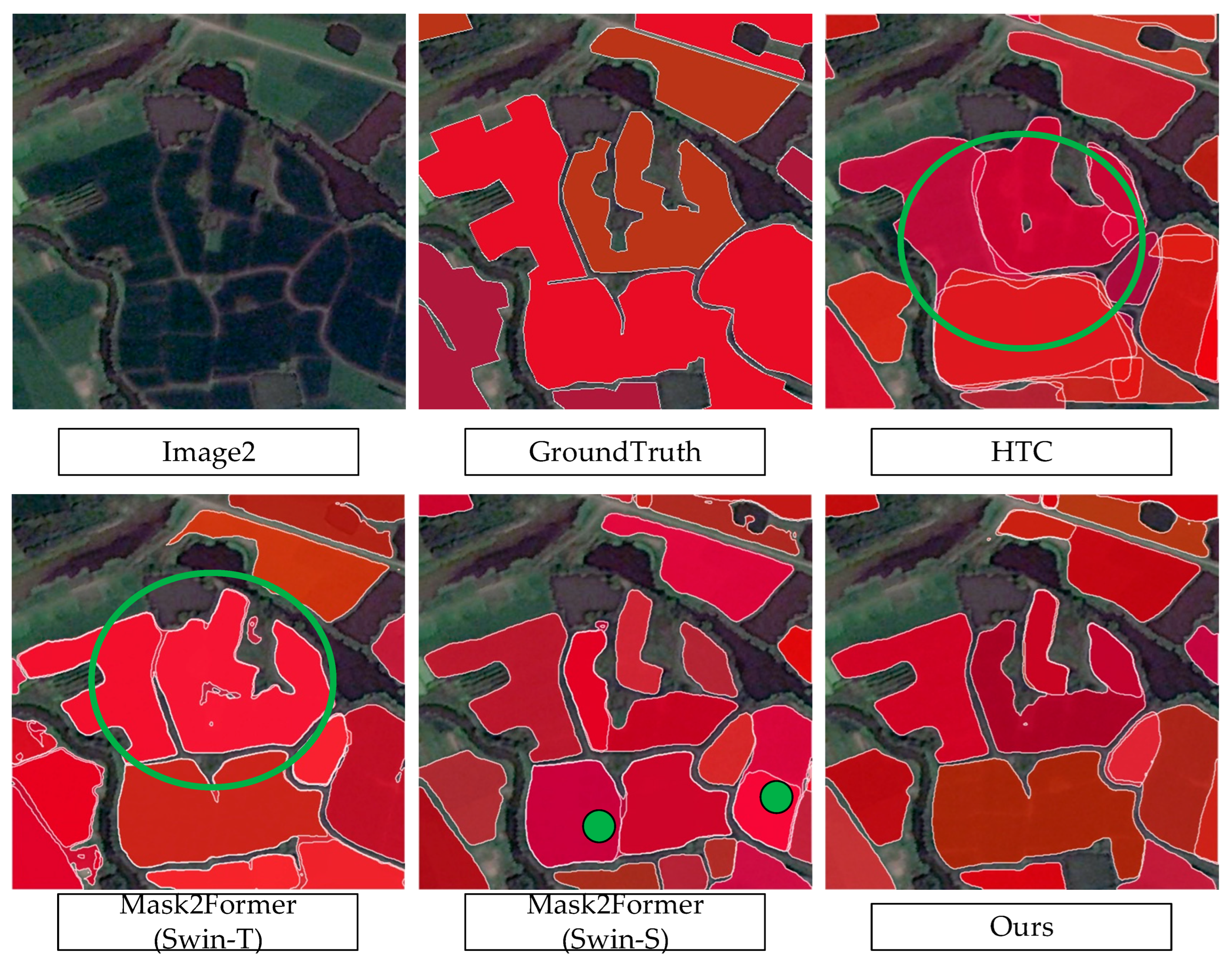
3.2. Visual Comparison

Since the quantitative comparison of these models shows very little difference, the visual difference better represents the results. Subsequently, a visual comparison is designed and the results are shown in Figure 7, Figure 8 and Figure 9. HTC (integrated with the FPN DCN module) is the champion in the competition held in 2021. Our baseline MaskFormer is the SOTA model in the COCO dataset, and the backbones employing Swin-T and Swin-S, respectively, are also shown in the visual comparisons.

Figure 7 shows an example with very large-sized fields. It can be found that the HTC cannot identify the fields of very large size, but the others are quite good at this. Among the networks, our proposed network shows the best segmentation. In addition, the fields have different planting status. The yellow and brown fields are the unplanted bare soil and the green ones are the planted areas. It seems that the HTC finds it difficult to identify the planted fields. Although some of the planted ones are identified, the boundaries are far from the the ground truth. MaskFormer with Swin-T is a little better than HTC, but it still cannot identify most of the planted fields. However, MaskFormer with Swin-S and our proposed model are better at this, and our proposed model shows the best result. The segmentation differences are indicated using green circles and ellipses. Therefore, our proposed network is better for instance segmentation at multiple scales and it is also insensitive to the color of the instance, such as planted and unplanted fields.

From the comparison results of irregular fields in Figure 8, it can be found that HTC performs the worst. The fields’ boundaries overlap and they are very difficult to separate from one another. MaskFormer (Swin-T) contains many very small fields within large ones, and the small ones are clearly wrong. MaskFormer (Swin-S) and our model show better results, and our results are more complete. The pond at the bottom right is misidentified by all the networks except ours. Thus, the proposed network is more competent in the case of irregular fields.

In the comparison of dense and regular fields in Figure 9, HTC did not extract the information of small-scale fields. MaskFormer with both Swin-T and Swin-S show more overlapping effects, resulting in a poor visual effect. The two very small adjacent fields indicated with the yellow dot at the upper left corner were identified by our model only. Consequently, although all the models were good in the case of regular fields of very similar size, ours showed the best segmentation.

Based on the visual comparisons above, the segmentation differences are very large, although the quantitative difference looks small. HTC shows the worst results and our model shows the best results in all the three of the cases. Among the three cases, all the models show the best segmentation on the regular fields of similar size. None of the models, except ours, is good in the cases with very large size differences and irregular fields. Thus, the proposed model is very effective and has higher accuracy.

3.3. Multi-Scale Target Results

Due to the introduction of the idea of multi-scale parallelism, our model achieves better results at different scales of fields than baseline. Among the COCO instance segmentation evaluation indicators, there are three indicators (AP small, AP medium, and AP large) which are used to evaluate the sizes smaller than 32 × 32; 32 × 32~96 × 96; and over 96 × 96, respectively.

It can be found from the comparison in

Table 2. Results of case segmentation at different scales. Our improved network achieves good results at all scales. The maximum improvement is reflected in the Bounding Box AP Small, up 1.5 percentage points.

Model	Bounding Box AP			Segmentation AP
	Small	Medium	Large	Small	Medium	Large
Mask2Former (Swin-T-7)	0.210	0.554	0.636	0.198	0.546	0.656
Mask2Former (Swin-T-12)	0.210	0.554	0.626	0.195	0.531	0.650
Mask2Former (Swin-S-7)	0.195	0.553	0.623	0.187	0.541	0.657
Ours (5-7-11)	0.220	0.569	0.649	0.203	0.545	0.670

that simply changing the window size of different scales and using Swin-S (at the third stage, the number of blocks stacked is tripled) will not bring better results, especially after using S. All scales are harmful to the results, which indicates that simply lengthening the network will give the model worse generalization ability. The advantages of our multi-scale window parallel mechanism are fully reflected.

3.4. More Window Exploration

We also further explored the window parallel mechanism. Considering the large difference in the size distribution of the fields, we increased the number of windows in parallel to four to enable better adaptability in feature extraction. This resulted in the consumption of about 10 m parameters. Compared with the baseline, this result is slightly improved, which is shown in

Table 3. Results of parallel connection of four scale windows, our results are still higher than baseline, but lower than those of our previous model.

Model	AP (bbox)	AP50 (bbox)	AP75 (bbox)	AP (segm)	AP50 (segm)	AP75 (segm)	Param (M)
Mask2Former (Swin-T-7)	0.522	0.742	0.562	0.523	0.754	0.566	47.40
Mask2Former (Swin-T-12)	0.518	0.740	0.559	0.513	0.745	0.555	47.45
Mask2Former (Swin-S-7)	0.515	0.743	0.557	0.517	0.747	0.564	68.72
Ours (5-7-11-13)	0.527	0.748	0.570	0.525	0.759	0.569	73.49
Ours (5-7-12-16)	0.526	0.747	0.571	0.525	0.759	0.570	73.54
Ours (5-7-11)	0.535	0.749	0.583	0.527	0.758	0.575	64.76

, but it is lower than our original design of three parallel windows (this is consistent with the fact that the accuracy of Swin-S is lower than that of Swin-T). Therefore, the principle of moderation should be adopted in the number of parallel connections, which can be adjusted flexibly according to the size of the dataset.

4. Discussion

4.1. Overlapping Problem

From the comparison of experimental results, it can be seen that the MSMTransformer’s multi-scale window parallel mechanism has improved the indicators of COCO. Since the basic network used is an end-to-end instance segmentation network, it will inevitably bring about overlapping problems. DETR is the first end-to-end target detection network, and the detection task is regarded as a set prediction problem [27]. This new idea is simple and clear and, more importantly, it cuts the processes of the anchor and NMS. However, border overlapping between some adjacent objects is induced. On the one hand, the problem can be attributed to the incomplete feature map extracted by the backbone network, which cannot distinguish objects of different scales. On the other hand, the object queries [27] of the detection head do not have explicit mutual exclusion operation in the process of cross-attention. Therefore, this kind of end-to-end target detection network still has room for improvement in dense scenes. For convolutional neural networks, the development of multi-scale modules such as Feature Pyramid Networks (FPN) [36], Inception [28], Atrous Spatial Pyramid Pooling (ASPP) [37], etc., is very rapid but it has not been applied to the Transformer. In this paper, multi-scale feature extraction and a Transformer are used to improve the accuracy of case segmentation and alleviate the overlap effect of end-to-end networks (as shown in Figure 9).

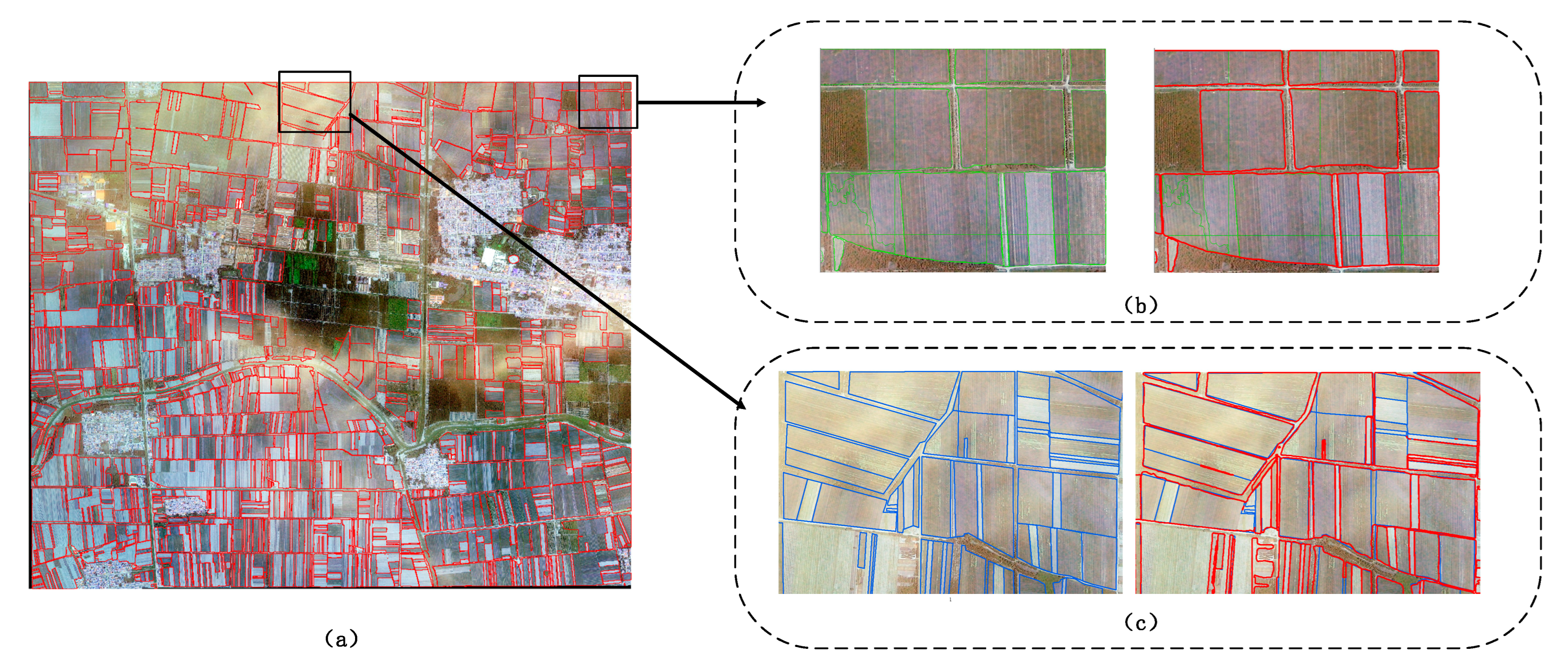
4.2. Merging the Outputted Small Images into One Single Vector File

In the field of computer vision, the results of instance segmentation are evaluated according to each small-sized image. In the field of remote sensing, the size of a remote sensing image is usually very large compared to the cropped input image. Because each large image is divided into a set of 512 × 512 small images, the outputs form the network are often not what we need. For example, many field extraction competitions require the contestants to submit a vector map corresponding to the size of the original image. It is very necessary to merge the outputs into a single vector file.

Two problems need to be solved in the process of merging all outputted small images. One is the overlapping problem mentioned above, that is, one area belongs to multiple field objects. The other is that one field is in two images due to truncation in the process of splitting small images. Here, we propose a buffer-based post-processing strategy. The whole process is divided into two stages. The first stage is to obtain overlapping vector files, and the second stage is to merge polygons based on the buffer. Figure 10 shows the complete process and the input of each operation more clearly. The process is described in detail as follows:

Step 1. For an original image, the partition is performed according to the overlapping strategy, so that there is a certain size of overlap between two adjacent small images (the size set in the experiment is 256). The small images with overlapping areas are then inputted into the model for prediction to achieve image segmentation. Subsequently, each small image is segmented in a fixed order, so the relative position is fixed. The model result is converted into a whole vector file according to its coordinates in the original large image. When a field is divided into two small images, the model can output two results with a certain degree of overlap; subsequently, the results are merged according to the subsequent merging strategy.

Step 2. The results from step 1 have many overlaps, part of which comes from the overlap strategy of small graph partition, and part of which comes from the overlap problem caused by the model itself. At this time, a simple consolidation strategy cannot be adopted, because the field dataset is very dense between fields, and the polygon objects outputted by the model will be adjacent or very close. If the two fields are merged directly, they are likely to be merged. Here, we propose a buffer-based shrinkage and expansion strategy. First, all polygonal objects are etched at a small distance. Because a large enough overlap area is reserved in step 1, a truncated field will still give overlapping results. Then, merge all polygons with overlap into one polygon, which can most probably ensure that a correct result is obtained for the field. However, due to the overlapping problem of the network itself, this operation will inevitably merge some fields that should not have been merged. Finally, inflate all new polygon objects to the same distance as above to recover the boundaries as predicted.

Figure 11a shows one of the remote sensing images and its corresponding merged results. In the figure, the blue lines indicate the ground truth from the official released dataset; the green lines indicate the initial retrieved fields before the merging process; the red lines indicate the final fields after the merging process. Therefore, Figure 11b shows an example of merged fields being better than the initial retrieved fields; Figure 11c shows that the final fields after post-processing still have some errors compared with the ground truth. The application of this post-processing strategy has achieved a very good field merging effect, although a few of overlapping fields still exist, as shown in Figure 11c.

5. Conclusions

In this paper, we propose an instance segmentation model called the MSMTransformer, which innovatively designs a multi-scale parallel shift-window structure (Multi-Swin block), and introduces the concept of multi-scale into the Swin Transformer to better extract features with largely different scales. The application of this model to field extraction has been very successful, not only bringing about the overall improvement of indicators, but also effectively alleviating the overlapping problem caused by the end-to-end instance segmentation framework. It proves that Transformer architecture has excellent performance in field extraction from remote sensing images, and the success of our model makes it possible to introduce more multi-scale modules into the Transformer.

References

1. Carfagna, E.; Gallego, F.J. Using remote sensing for agricultural statistics. Int. Stat. Rev. 2005, 73, 389–404. [Google Scholar] [CrossRef] [Green Version]
2. Graesser, J.; Ramankutty, N. Detection of cropland field parcels from Landsat imagery. Remote Sens. Environ. 2017, 201, 165–180. [Google Scholar] [CrossRef] [Green Version]
3. Johnson, D.M. A 2010 map estimate of annually tilled cropland within the conterminous United States. Agric. Syst. 2013, 114, 95–105. [Google Scholar] [CrossRef]
4. Rudel, T.K.; Schneider, L.; Uriarte, M.; Turner, B.L.; Grauj, R. Agricultural Intensification and Changes in Cultivated Areas. 2005. Available online: https://xueshu.baidu.com/usercenter/paper/show?paperid=c7de4819aa39593de58f99ec0510d8b6&site=xueshu_se&hitarticle=1 (accessed on 2 December 2022).
5. Taravat, A.; Wagner, M.P.; Bonifacio, R.; Petit, D. Advanced Fully Convolutional Networks for Agricultural Field Boundary Detection. Remote Sens. 2021, 13, 722. [Google Scholar] [CrossRef]
6. Fw, A.; Fid, B. Deep learning on edge: Extracting field boundaries from satellite images with a convolutional neural network—ScienceDirect. Remote Sens. Environ. 2020, 245, 111741. [Google Scholar]
7. De Wit, A.J.W.; Clevers, J.G.P.W. Efficiency and accuracy of per-field classification for operational crop mapping. International J. Remote Sens. 2004, 25, 4091–4112. [Google Scholar] [CrossRef]
8. Canny, J. A computational approach to edge detection. IEEE Trans. Pattern Anal. Mach. Intell. 1986, PAMI-8, 679–698. [Google Scholar] [CrossRef]
9. Hong, R.; Park, J.; Jang, S.; Shin, H.; Song, I. Development of a Parcel-Level Land Boundary Extraction Algorithm for Aerial Imagery of Regularly Arranged Agricultural Areas. Remote Sens. 2021, 13, 1167. [Google Scholar] [CrossRef]
10. Cheng, T.; Ji, X.; Yang, G.; Zheng, H.; Ma, J.; Yao, X.; Zhu, Y.; Cao, W. DESTIN: A new method for delineating the boundaries of crop fields by fusing spatial and temporal information from WorldView and Planet satellite imagery—ScienceDirect. Comput. Electron. Agric. 2020, 178, 105787. [Google Scholar] [CrossRef]
11. Uijlings, J.R.; Sande, K.E.; Gevers, T.; Smeulders, A.W. Selective Search for Object Recognition. Int. J. Comput. Vis. 2013, 104, 154–171. [Google Scholar] [CrossRef] [Green Version]
12. Soille, P.J.; Ansoult, M.M. Automated basin delineation from digital elevation models using mathematical morphology. Signal Process. 1990, 20, 171–182. [Google Scholar] [CrossRef]
13. Hossain, M.; Chen, D. Segmentation for Object-Based Image Analysis (OBIA): A review of algorithms and challenges from remote sensing perspective. ISPRS J. Photogramm. Remote Sens. 2019, 150, 115–134. [Google Scholar] [CrossRef]
14. Watkins, B.; Niekerk, A.V. A comparison of object-based image analysis approaches for field boundary delineation using multi-temporal Sentinel-2 imagery. Comput. Electron. Agric. 2019, 158, 294–302. [Google Scholar] [CrossRef]
15. Long, J.; Shelhamer, E.; Darrell, T. Fully Convolutional Networks for Semantic Segmentation. IEEE Trans. Pattern Anal. Mach. Intell. 2017. [Google Scholar] [CrossRef]
16. He, K.; Gkioxari, G.; Dollar, P.; Girshick, R. Mask R-CNN. In Proceedings of the International Conference on Computer Vision, Venice, Italy, 22–29 October 2017. [Google Scholar] [CrossRef]
17. Cheng, B.; Misra, I.; Schwing, A.G.; Kirillov, A.; Girdhar, R. Masked-attention Mask Transformer for Universal Image Segmentation. arXiv 2021, arXiv:2112.01527. [Google Scholar]
18. Wang, D.; Liu, Z.; Gu, X.; Wu, W.; Chen, Y.; Wang, L. Automatic Detection of Pothole Distress in Asphalt Pavement Using Improved Convolutional Neural Networks. Remote Sens. 2022, 14, 3892. [Google Scholar] [CrossRef]
19. Liu, Z.; Gu, X.; Chen, J.; Wang, D.; Chen, Y.; Wang, L. Automatic recognition of pavement cracks from combined GPR B-scan and C-scan images using multiscale feature fusion deep neural networks. Autom. Constr. 2023, 146, 104698. [Google Scholar] [CrossRef]
20. Han, K.; Wang, Y.; Chen, H.; Chen, X.; Guo, J.; Liu, Z.; Tang, Y.; Xiao, A.; Xu, C.; Xu, Y. A Survey on Vision Transformer. IEEE Trans. Pattern Anal. Mach. Intell. 2022. [Google Scholar] [CrossRef] [PubMed]
21. Chen, Y.; Gu, X.; Liu, Z.; Liang, J. A Fast Inference Vision Transformer for Automatic Pavement Image Classification and Its Visual Interpretation Method. Remote Sens. 2022, 14, 1877. [Google Scholar] [CrossRef]
22. Li, X.; Xu, F.; Xia, R.; Li, T.; Chen, Z.; Wang, X.; Xu, Z.; Lyu, X. Encoding Contextual Information by Interlacing Transformer and Convolution for Remote Sensing Imagery Semantic Segmentation. Remote Sens. 2022, 14, 4065. [Google Scholar] [CrossRef]
23. Yang, L.; Yang, Y.; Yang, J.; Zhao, N.; Wu, L.; Wang, L.; Wang, T. FusionNet: A Convolution–Transformer Fusion Network for Hyperspectral Image Classification. Remote Sens. 2022, 14, 4066. [Google Scholar] [CrossRef]
24. Zhao, Z.; Liu, Y.; Zhang, G.; Tang, L.; Hu, X. The Winning Solution to the iFLYTEK Challenge 2021 Cultivated Land Extraction from High-Resolution Remote Sensing Image. In Proceedings of the 2022 14th International Conference on Advanced Computational Intelligence (ICACI), Wuhan, China, 15–17 July 2022. [Google Scholar] [CrossRef]
25. Kai, C.; Pang, J.; Wang, J.; Yu, X.; Lin, D. Hybrid Task Cascade for Instance Segmentation. In Proceedings of the IEEE/CVF Conference on Computer Vision & Pattern Recognition, Long Beach, CA, USA, 15–20 June 2019. [Google Scholar] [CrossRef]
26. Cai, Z.; Vasconcelos, N. Cascade R-CNN: Delving into High Quality Object Detection. arXiv 2017, arXiv:1712.00726. [Google Scholar] [CrossRef]
27. Nicolas, C.; Francisco, M.; Gabriel, S.; Nicolas, U.; Alexander, K.; Sergey, Z. End-to-End Object Detection with Transformers. arXiv 2020, arXiv:2005.12872. [Google Scholar]
28. Szegedy, C.; Liu, W.; Jia, Y.; Sermanet, P.; Reed, S.; Anguelov, D.; Erhan, D.; Vanhoucke, V.; Rabinovich, A. Going Deeper with Convolutions. In Proceedings of the 2015 IEEE Conference on Computer Vision and Pattern Recognition (CVPR), Boston, MA, USA, 7–12 May 2015; pp. 1–9. [Google Scholar] [CrossRef]
29. Lin, T.Y.; Maire, M.; Belongie, S.; Hays, J.; Zitnick, C.L. Microsoft COCO: Common Objects in Context. In European Conference on Computer Vision; Springer: Cham, Switzerland, 2014; pp. 740–755. [Google Scholar] [CrossRef] [Green Version]
30. Dosovitskiy, A.; Beyer, L.; Kolesnikov, A.; Weissenborn, D.; Houlsby, N. An Image is Worth 16 × 16 Words: Transformers for Image Recognition at Scale. arXiv 2020, arXiv:2010.11929. [Google Scholar]
31. Liu, Z.; Lin, Y.; Cao, Y.; Hu, H.; Wei, Y.; Zhang, Z.; Lin, S.; Guo, B. Swin Transformer: Hierarchical Vision Transformer using Shifted Windows. arXiv 2021, arXiv:2103.14030. [Google Scholar]
32. Technicolor, T.; Related, S.; Technicolor, T.; Related, S. ImageNet Classification with Deep Convolutional Neural Networks; ACM: New York, NY, USA, 2012; Volume 60, pp. 84–90. [Google Scholar]
33. Luo, W.; Li, Y.; Urtasun, R.; Zemel, R. Understanding the Effective Receptive Field in Deep Convolutional Neural Networks. arXiv 2017, arXiv:1701.04128. [Google Scholar]
34. Vaswani, A.; Shazeer, N.; Parmar, N.; Uszkoreit, J.; Jones, L.; Gomez, A.N.; Kaiser, L.; Polosukhin, I. Attention Is All You Need. arXiv 2017, arXiv:1706.03762. [Google Scholar]
35. Liu, Z.; Yeoh, J.K.W.; Gu, X.; Dong, Q.; Chen, Y.; Wu, W.; Wang, L.; Wang, D. Automatic pixel-level detection of vertical cracks in asphalt pavement based on GPR investigation and improved mask R-CNN. Autom. Constr. 2023, 146, 104689. [Google Scholar] [CrossRef]
36. Lin, T.Y.; Dollar, P.; Girshick, R.; He, K.; Hariharan, B.; Belongie, S. Feature Pyramid Networks for Object Detection. In Proceedings of the 2017 IEEE Conference on Computer Vision and Pattern Recognition (CVPR), Honolulu, HI, USA, 21–26 July 2017. [Google Scholar] [CrossRef]
37. Chen, L.C.; Papandreou, G.; Kokkinos, I.; Murphy, K.; Yuille, A.L. DeepLab: Semantic Image Segmentation with Deep Convolutional Nets, Atrous Convolution, and Fully Connected CRFs. IEEE Trans. Pattern Anal. Mach. Intell. 2018, 40, 834–848. [Google Scholar] [CrossRef]
Figure 1. (a) One of the original images and its corresponding labels provided with the original dataset. (b) The visualization result after conversion of the dataset to COCO format with its size fixed at 512 × 512.
Remotesensing 15 00549 g001
Figure 2. The field area is counted according to three scales: small, medium, and large. The proportion of fields of each scale is about 1:3:2.
Remotesensing 15 00549 g002
Figure 3. The overall architecture of the MSMTransformer and image merging process. The purple area is the Multi-Swin Transformer block, which is used to extract multi-scale information.
Remotesensing 15 00549 g003
Figure 4. The Multi-Swin Transformer block is built by replacing the multi-head self-attention modules that have a regular (shift) window (W-MSA, SW-MSA) with a multi-scale (shift) window parallel module (MW-MSA, SMW-MSA). The LayerNorm (LN) and Multi-Layer Perceptron (MLP) are applied to the block.
Remotesensing 15 00549 g004
Figure 5. Schematic of multi-scale window based multi-head self-attention (MW-MSA) module. The windows of different sizes are designed to extract fields with different scales. Q. K and V are operation elements of self-attention. The design of the SMW-MSA module is the same.
Remotesensing 15 00549 g005
Figure 6. Network architecture of the MSMTransformer and the layer settings.
Remotesensing 15 00549 g006
Figure 7. Visualization results of different models on fields with large-scale transformation. Green circles highlight areas of poor extraction.
Remotesensing 15 00549 g007
Figure 8. Visual comparison of different models for segmenting irregular fields. Green circles highlight areas of poor extraction.
Remotesensing 15 00549 g008
Figure 9. Visual comparison of different models on regular fields of similar size. Green circles highlight areas of poor extraction. Yellow circles highlight areas of small-scale fields in groundtruth.
Remotesensing 15 00549 g009
Figure 10. A flowchart for post-processing of merged fields from instance segmentation into a single vector file. The input is a large-sized remote sensing image and the output is the corresponding vector file.
Remotesensing 15 00549 g010
Figure 11. Full image output after post-processing and some of the zoomed-in details. (a) The original remote sensing image and the results obtained by our network through post-processing. (b,c) Detail drawing of local area.
Remotesensing 15 00549 g011