Optimizing Back-Propagation Neural Network to Retrieve Sea Surface Temperature Based on Improved Sparrow Search Algorithm

Abstract

Sea surface temperature (SST) constitutes a pivotal physical parameter in the investigation of atmospheric, oceanic, and air–sea exchange processes. The retrieval of SST through satellite passive microwave (PMW) technology effectively mitigates the interference posed by cloud cover, addressing a longstanding challenge. Nevertheless, conventional functional representations often fall short in capturing the intricate interplay of factors influencing SST. Leveraging neural networks (NNs), known for their adeptness in tackling nonlinear and intricate problems, holds great promise in SST retrieval. Nonetheless, NNs exhibit a high sensitivity to initial weights and thresholds, rendering them susceptible to local optimization issues. In this study, we present a novel machine learning (ML) approach for SST retrieval using PMW measurements, drawing from the Sparrow Search Algorithm (SSA) and Back-Propagation neural network (BPNN) methodologies. The core premise involves the optimization of the BP neural network’s initial weights and thresholds through an enhanced SSA algorithm employing various optimization strategies. This optimization aims to provide superior parameters for the training of the BP neural network. Employing AMSR2 brightness temperature data, sea surface wind speed data, and buoy SST measurements, we construct the ISSA-BP model for sea surface temperature retrieval. The validation of the ISSA-BP model against the test data is conducted and compared against the multiple linear regression (MLR) model, an unoptimized BP model, and an unimproved SSA-BP model. The results manifest an impressive R-squared (R²) value of 0.9918 and a root-mean-square error (RMSE) of 0.8268 °C for the ISSA-BP model, attesting to its superior accuracy. Furthermore, the ISSA-BP model was applied to retrieve global sea surface temperatures on 15 July 2022, yielding an R² of 0.9926 and an RMSE of 0.7673 °C for the OISST product on the same day, underscoring its excellent concordance. The results indicate that SST can be efficiently and accurately retrieved using the model proposed in this paper, based on satellite PMW measurements. This finding underscores the potential of employing machine learning algorithms for SST retrieval and offers a valuable reference for future studies focusing on the retrieval of other sea surface parameters.

1. Introduction

Oceans constitute a pivotal component of the Earth’s hydrosphere, encompassing approximately 71% of the planet’s surface. They serve as the primary absorber of solar radiation on a global scale, functioning as a crucial conduit for atmospheric energy propagation. Variations in sea temperature wield significant influence over local weather patterns and can induce discernible alterations in the global environment [1].

Sea surface temperature (SST), denoting the thermal state of the water immediately adjacent to the ocean’s surface, encapsulates the intricate interplay between oceanic and atmospheric dynamics. Its fluctuations signify exchanges of atmospheric heat, movements of ocean currents, and manifestations of climate change, among other phenomena. SST emerges as a paramount parameter in the realm of global oceanography and climate research [2], and the quest to measure SST boasts a legacy exceeding 150 years. Early SST measurements primarily relied upon shipborne and buoy-based observations [3]. However, these methods fell short of satisfying the demands of large-scale, real-time monitoring. Satellite remote sensing technology has emerged as a transformative tool, offering expansive coverage, high spatial resolution, and prolonged, repetitive observations, thus earning its ubiquitous role in global SST monitoring endeavors [4]. Satellite-based SST monitoring predominantly employs infrared (IR) and passive microwave (PMW) remote sensing techniques. While IR methods offer superior spatial resolution, they falter in the presence of cloud cover and are susceptible to daily fluctuations in solar radiation, atmospheric water vapor content, and aerosol conditions [5]. In contrast, PMW techniques surmount the aforementioned limitations of IR methods, facilitating all-weather observations, albeit at the cost of reduced spatial resolution and sensitivity to variations in sea surface roughness, primarily induced by high wind velocities [6].

Currently, common methods for retrieving SST from PMW measurements are statistical algorithms and physical algorithms. Statistical algorithms are used to calculate the corresponding parameters based on relationships obtained directly from the regression of synchronized observations of ships or buoys with satellites. Milman et al. carried out a retrieval study of SST based on measurements from the first satellite-borne scanning microwave radiometer, SMMR, and proposed a statistical regression retrieval method for ocean parameters [7]. Wenz et al. [8] established a statistical regression retrieval algorithm in logarithmic form for the SSM/I and AMSR microwave radiometers. Hao et al. [9] used AMSR-E microwave data and MODIS optical data to retrieve SST in the Northern Indian Ocean through multiple linear regression. The root-mean-square error (RMSE) between the retrieval results and the in situ SST was 0.32 °C. The physical algorithms were based on radiative transfer modeling, which requires consideration of all influential physical mechanisms during microwave emission and microwave transmission at the sea surface. All sea–air parameters that would have an impact on the measurement of the microwave signal are also considered. Shibata et al. [10] corrected the effect of wind speed in the algorithm to improve the accuracy of sea surface temperature retrieval. Wang et al. retrieved the SST with an RMSE of 0.73 K using the radiative transfer method [11].

Although many scholars have conducted extensive research on SST retrieval through PMW remote sensing and achieved fruitful results, there are still many problems in the retrieval process. Firstly, the retrieval models used in these studies are often designed for specific sea areas, making them inapplicable on a global scale and lacking portability. Secondly, the derivation of coefficients for these retrieval models mostly relies on the traditional statistical regression method, which is cumbersome. Machine learning (ML) algorithms exhibit enhanced flexibility in discerning intricate patterns and structures within complex problem domains when compared to traditional physical and statistical algorithms. It was found that ML has the potential to enhance existing PMW SST retrieval algorithms. A neural network (NN) is a system inspired by biological neural networks, typically comprising multilayers of neurons connected by weights that can be iteratively optimized by combining error back-propagation and gradient-based optimization. This process allows the system to approximate the underlying relationship between its inputs and outputs. Compared to linear fitting, a neural network has much stronger fitting capabilities when the data relationship is nonlinear, making it very useful for oceanic satellite retrievals [12,13]. Krasnopolsky et al. [14] employed an NN approach to simultaneously obtain wind speed, column water vapor, column liquid water, and SST using brightness temperatures from SSM/I. Lei Meng et al. [15] utilized SSM/I observations of brightness temperature to retrieve sea surface parameters using an NN, with the RMSE between the retrieved and measured values of SST being 1.54 °C. Emy Alerskans et al. [16] evaluated the ability of a multilayer perceptron neural network machine learning model for retrieving SST and demonstrated that the neural network machine learning approach has a great potential for inverting sea surface temperature in PMW satellite observations. However, neural networks are applied in a process where the initial weights and thresholds of the neural network are assigned randomly, and different initial values have a large impact on the prediction results [17]. The Sparrow Search Algorithm (SSA) takes into account all the possible factors of the group’s behavior, allowing it to quickly converge to the neighborhood of the optimum [18,19]. Therefore, this paper proposes a machine learning model based on the Improved Sparrow Search Algorithm (ISSA) to optimize the Back-Propagation neural network (BPNN) for SST retrieval. A novel swarm intelligence optimization algorithm is used to optimize the performance of the widely used BPNN model, which improves the optimization efficiency and accuracy of the BPNN. The experimental results demonstrate that, when compared with the common multiple linear regression and BPNN methods, the method proposed in this paper achieves higher accuracy in SST retrieval. The SSTs retrieved using the model presented in this paper also exhibit good agreement with the commonly available SST products today.

2. Data and Preprocessing

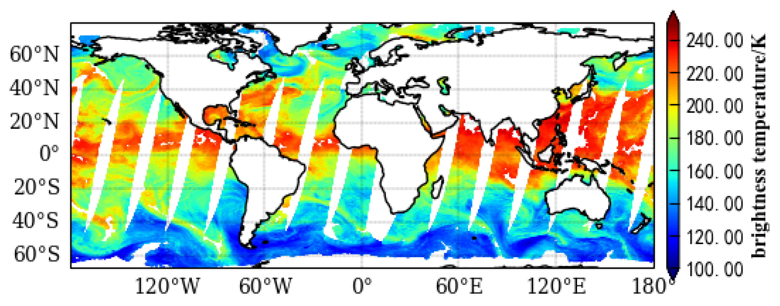
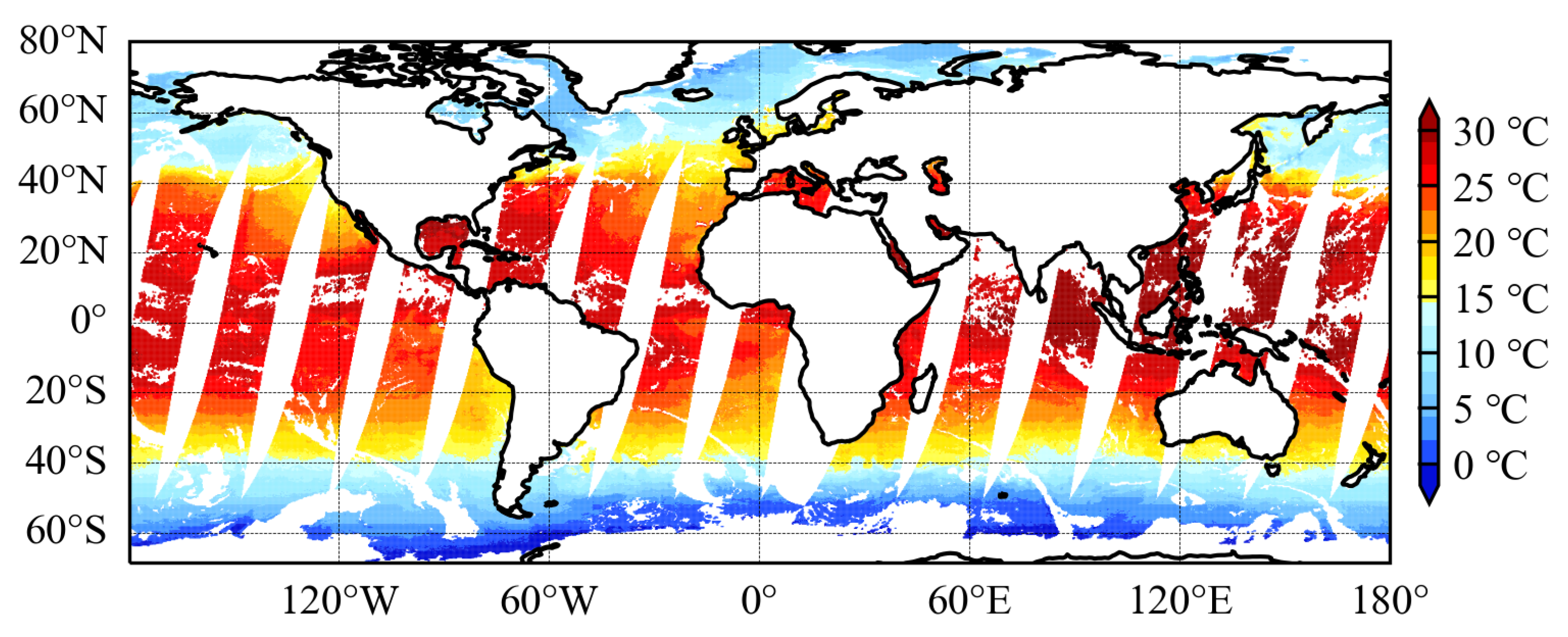
2.1. Data Presentation

The basis for the development of the retrieval algorithm proposed in this paper is the Multisensor Matchup Dataset (MMD) established in the European Space Agency’s (ESA) Climate Change Initiative project [20,21]. The MMD has been constructed as a generalized dataset for algorithm development rather than a dataset dedicated to a specific algorithm [22]. The MMD is available from the Center for Environmental Data Archives (CEDA) at https://gws-access.jasmin.ac.uk/public/esacci-sst/matchup_data/, accessed on 20 November 2022. The MMD data type we use is the matching data of the AMSR2 brightness temperature data, ERA5 wind speed data, and ARGO buoy data.

The AMSR2 sensor is an advanced cone-scanning microwave radiometer aboard the Global Change Observation Mission-1 Water (GCOM-W1) satellite. AMSR2 commenced real-time global surface microwave brightness temperature observations in July 2012, succeeding the AMSR-E microwave radiometer, which ceased operations in October 2011. It is considered a tool for measuring weak microwave emissions from the surface of the atmosphere and the surface of the Earth [23]. AMSR2 is about 700 km above the Earth, and its antenna rotates every 1.5 s to capture remote sensing data over 1450 km, giving it a global set of data every two days. It measures brightness temperatures at 6.9 GHz, 7.3 GHz, 10.7 GHz, 18.7 GHz, 23.8 GHz, 36.5 GHz, and 89.0 GHz at both horizontal and vertical polarizations. For sea surface temperature, the low-frequency channel is significantly more sensitive than the medium and high frequencies. Specifically, within the microwave frequency range of 4–8 GHz, the dielectric constant for water changes with physical temperature, resulting in emissivity values changing by up to ~50%. A recent study has indicated that the 6.9 GHz vertically polarized frequency channel’s brightness temperature data exhibit the highest sensitivity to SST [24]. In the retrieval of SST, it was necessary to include the 10.7 GHz channel’s brightness temperature in addition to the 6.9 GHz data to eliminate radio-frequency interference (RFI)-contaminated brightness temperatures. While higher-frequency (18.7–36.5 GHz) brightness temperatures are not very sensitive to changes in SST, they provide important information about the near-surface atmosphere and thus need to be incorporated into the retrieval algorithm. For instance, the water vapor content of the atmosphere can affect the penetration of microwave radiation. Alsweiss et al. [25] subsequently developed an SST retrieval algorithm utilizing AMSR2’s 12 frequency channels of brightness temperatures (6.9–36.5 GHz). Studies have also identified the four optimal frequencies (6.9, 7.3, 10.7, and 36.5 GHz) of AMSR2 for SST retrievals [26]. In order to fully leverage the information contained in all AMSR2 channels, we utilized 14 channels from 6.9 to 89.0 GHz to retrieve SST in this study. Figure 1 shows a schematic diagram of the brightness temperatures for horizontal polarization at 23.8 GHz. The detailed parameters of the AMSR2 sensor are given in

Table 1. Main technical parameters of AMSR2.

Frequency (GHz)	Resolution (km × km)	Polarization Mode	Incidence Angle	Swath Width
6.9	62 × 35	Horizontal and vertical polarization	55°	1450 km
7.3	62 × 35
10.7	42 × 24
18.7	22 × 14
23.8	19 × 11
36.5	12 × 7
89.0	5 × 3

.

ARGO buoys constitute a globally distributed array of drifting buoys, enabling real-time monitoring of ocean temperature and salinity profiles, as well as water depth within the 0 to 2000 m range. These buoys also track their movement trajectories to deduce seawater speed and direction. Positioned at intervals of approximately 300 km, each buoy autonomously surfaces every 10 days, transmitting precise temperature and salinity profiles, along with positional data, to terrestrial receiving stations via satellite links. The temperature measurement range of the ARGO buoy spans from −3 to 32 °C, boasting an impressive measurement accuracy within a range of ±0.005 °C [27]. Within the framework of the MMD, satellite-measured brightness temperatures are temporally and spatially synchronized with the measured data. The matching criteria involve identifying valid satellite data points within a 0.2° × 0.2° radius centered on the actual data point. Furthermore, the time constraint stipulates that the time of observation for the actual point and the detection time of the satellite point should not differ by more than 4 h. Additional data included in the MMD are information from both the ERA-Interim reanalysis [28] and the ERA5 reanalysis [29] on SST, total column water vapor (TCWV), total cloud liquid water (TCLW), wind speed (WS), and sea ice concentration (SIC). Previous studies have demonstrated that the uncertainty in retrieved SST increases at higher wind speeds [20]. The sensitivity of brightness temperature to wind speed increases with higher wind speeds (i.e., surface roughness) and when white foam appears on the surface, which may be related to surface roughness and physical properties [30]. Therefore, the wind speed data in the MMD were chosen to be added to the matched data created.

2.2. Preprocessing

In order to ensure the precision of the retrieval algorithm, it is imperative to conduct fundamental data quality control within the Multiple Microwave Data (MMD) dataset prior to algorithm development. The initial step involves the elimination of abnormal brightness temperature values. In this study, it has been determined that the valid range for brightness temperatures falls within 70–320 K. Consequently, any AMSR2 observations of brightness temperature data falling outside this specified range have been systematically excluded from our dataset. Following the criteria laid out by Wu and Weng in 2011 [31], the brightness temperature data from AMSR2 underwent a processing step utilizing 6.9 GHz and 10.7 GHz brightness temperature measurements to alleviate the effects of radio frequency interference (RFI) contamination.

$$\mathrm{RFI}=\mathrm{Tb}\left(6.9\mathrm{GHz}\right)-\mathrm{Tb}\left(10.7\mathrm{GHz}\right)>5\mathrm{K}.$$

(1)

In addition, rainfall-affected AMSR2 data (18.7 GHz vertically polarized channel greater than 240 K) are to be excluded, as the microwave scattering effect due to precipitation particles can have a large impact on the SST retrieval results. Data were excluded if the difference between the vertical and horizontal polarizations for the 18–36 GHz brightness temperatures was negative, as this indicates invalid oceanographic retrievals. In situ data outside the range of −2–34 °C were also excluded, with the lower limit of −2 °C applied to eliminate matchups potentially contaminated by sea ice. Additional checks are necessary, as both atmospheric and surface effects can contaminate the signal and lead to erroneous retrievals. Sea ice and land affect retrieval due to antenna side-lobe contamination. Furthermore, matchups with a sea surface wind speed greater than 15 m/s were removed. The upper wind speed limit is based on the fact that extreme surface roughness and the existence of foam on the surface caused by high wind speeds impact brightness temperatures and make SST retrievals uncertain [30].

In this paper, the July and August 2016 matched datasets were selected for the retrieval study, and 14,252 sets of valid matches were used. Differences in input element scales and substantial variations in data scales can increase the complexity of model training. Therefore, data standardization plays a crucial role in the preprocessing of retrieved data before inputting them into the retrieval model. This process aligns the data’s outline and magnitude to create a more reasonable data distribution suitable for training retrieval models. We employed standard deviation standardization, also known as z-score standardization, which relies on the mean and standard deviation values of the original data. The standardized data follow a normal distribution with a mean of zero and a standard deviation of one. The formula for this process is as follows:

$$z=\frac{x-\mu }{\sigma },$$

(2)

where z represents the normalized data, x represents the original data, µ is the mean of the original dataset, and σ is the standard deviation of the original dataset.

3. Methods

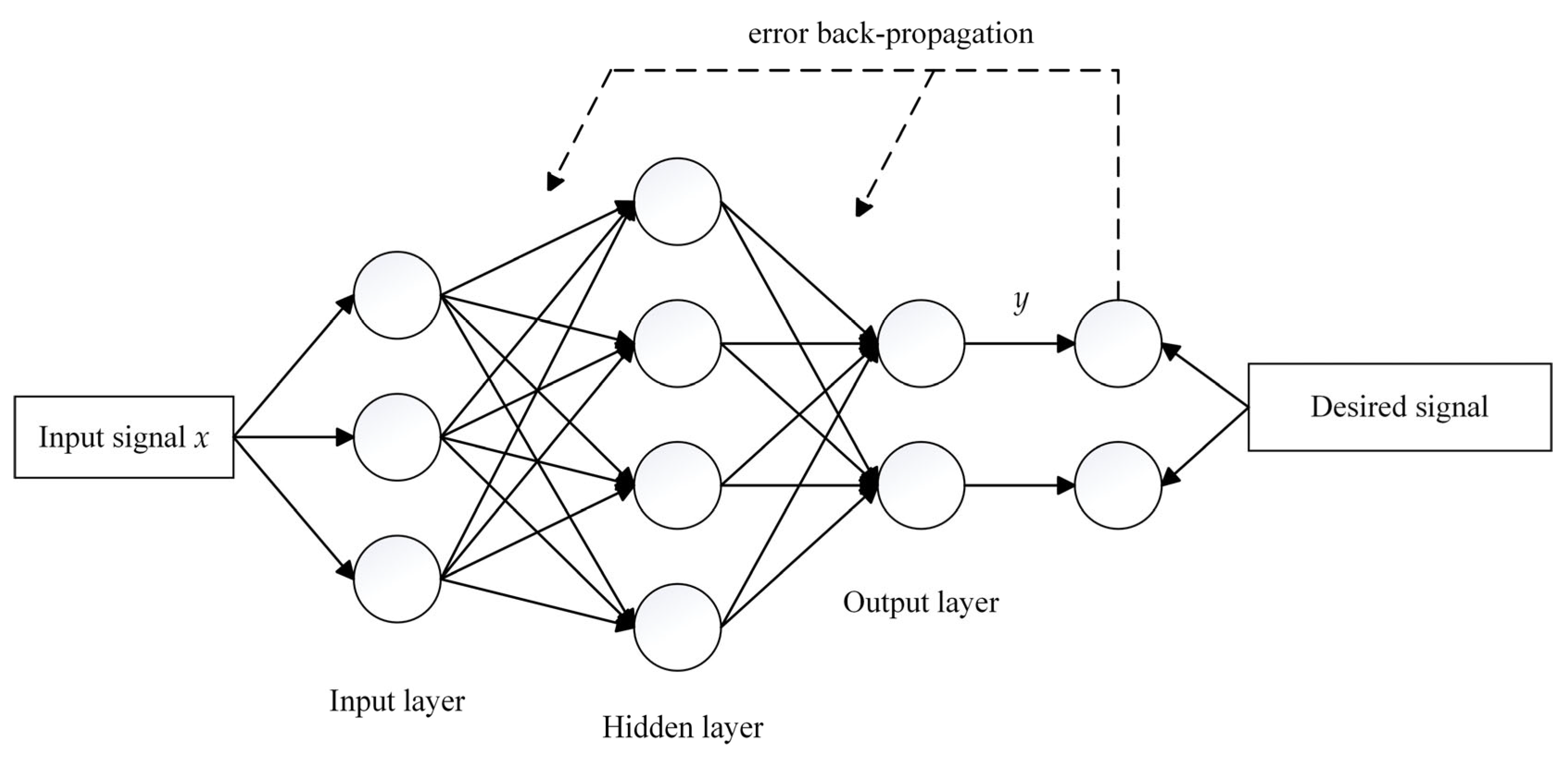
3.1. BP Neural Network

The Back-Propagation (BP) neural network is a multilayer feed-forward network trained using the error back-propagation algorithm, which was first proposed by scientists led by Rumelhart and McClelland in 1986 [32]. Its simple structure has found applications in a wide range of fields. The BP neural network comprises three layers: the input layer, the hidden layer(s), and the output layer. It operates on the principles of forward information propagation and backward error correction. External information enters through the input layer, undergoes processing and transmission within each neuron of the hidden layer(s), and, eventually, the output layer produces the results of information processing, completing the forward propagation of information. If the output information does not match the actual results or falls outside an acceptable error range, all weights and thresholds are adjusted following the “gradient descent” principle. Multiple iterations of forward and back-propagation can be performed until the error reaches an acceptable range or a predetermined number of learning cycles is completed. The structure of the BP neural network is depicted in Figure 2, and it can consist of one or more hidden layers.

Typically, the BP neural network model is a nonlinear function model in which the input values represent independent variables while the output values represent dependent variables of the function. In the prediction model, the input values correspond to the processed data samples, and the output values correspond to the corresponding predictions. When there are n input nodes and m output nodes, the prediction model captures the functional mapping relationship from n independent variables, denoted as “x”, to m dependent variables, resulting in the prediction results represented as “y”.

3.2. Sparrow Search Algorithm (SSA)

The Sparrow Search Algorithm (SSA) is the latest swarm optimization algorithm, introduced by Xue et al. in 2020 [19]. This algorithm draws its main inspiration from sparrows’ foraging and anti-predation behaviors, and it boasts strong optimization capabilities, rapid convergence, and high stability. SSA classifies sparrow flocks into distinct roles based on their foraging processes. Within these flocks, there are “finders” with superior adaptive values responsible for identifying shared foraging areas and exploring new directions. Meanwhile, “followers” rely on the finders to locate food and follow suit. Additionally, a portion of the sparrow flock is tasked with scouting during foraging. If the warning threshold surpasses the safety threshold, the flock decides to abandon the food source, establishing an early warning mechanism during foraging. Based on these principles, it becomes evident that position plays a crucial role in guiding the behavior of the sparrow flock. The algorithmic flow of the Sparrow Search Algorithm has been summarized in the following subsections.

3.2.1. Determine the Fitness Value of Each Position

The sparrow population is represented by an n × d dimensional matrix X, where d is the dimension of the variable to be optimized and n is the number of sparrows. Then, the initial position of the sparrows is as in Formula (3):

$$X=\left[\begin{array}{cccc}{x}_{11}& x_{12}& \cdots & x_{1d}\\ x_{21}& x_{22}& \cdots & x_{2d}\\ ⋮& ⋮& \ddots & ⋮\\ x_{n1}& x_{n2}& \cdots & x_{nd}\end{array}\right].$$

(3)

The fitness value F of the sparrow population is expressed as Formula (4):

$$F=[f\left(X_1\right),f\left(X_2\right)\cdots f\left(X_n\right){]}^{\mathrm{T}} ,$$

(4)

where F is the fitness function, $X_i$ is the position of the ith sparrow, and $f\left(X_i\right)$ is the fitness value of the ith individual sparrow. During the foraging process, the location of the sparrow with a high fitness value indicates that the food in this area will attract other sparrows to forage. Sparrows with high fitness values become the finders of the population, leading the foraging and movement direction of the population.

3.2.2. Updating Finder Locations

Finders can locate food and guide populations during migration, enabling them to forage over a wider range compared to other sparrows. In each iteration, the position of the finder is updated as follows:

$$X_{i,j}^{t+1}=\left\{\begin{array}{c}{X}_{i,j}^t·\mathit{exp}\left(\frac{-i}{\alpha ·ie{r}_{max}}\right),R_2<ST\hfill \\ X_{i,j}^t+Q,{ R}_2\ge ST \end{array}\right. ,$$

(5)

where α is a uniform random number with a range of (0, 1]; Q is a standard normally distributed random number; $X_{i,j}^{t+1}$ represents the new position of the t generation in the population; $R_2$ is the warning value, and the range is [0, 1]; and ST is a safe value. When $R_2$ is greater than ST, the sparrow will randomly move to the safe position according to the normal distribution and gradually converge to the optimal position. When $R_2$ is less than ST, there is no predator threat, and the finder will move in the optimized direction.

3.2.3. Update Follower Position

The follower’s position moves with the finder. When the finder finds food in a better location, the follower abandons its current position and flies around the finder to feed. The follower position is updated as follows:

$$X_{i,j}^{t+1}=\left\{\begin{array}{c}Q·exp\left(\frac{X_{worst}-X_{i,j}^t}{i^2}\right),i>n/2\\ X_p^{t+1}+| X_{i,j}^t-X_p^{t+1} |· A^{+}·L,i\le n/2 \end{array}\right.,$$

(6)

where t is the number of iterations; $X_{worst}$ indicates the current worst position in the sparrow flock; $X_p^{t+1}$ represents the best position of the sparrow group; A is a 1 × d matrix (random numbers with values of 1 and −1); and $A^{+}$ = A^T (AA^T)⁻¹. When i > n/2, it means that the ith follower with the worst adaptation needs to immediately go to other places to forage for food because it did not acquire food. When i ≤ n/2, it means that the ith follower is searching for food at a specific location near the best location $X_p^{ }$.

3.2.4. Detection and Early Warning

A typical 15 to 30 percent of a sparrow flock goes to watch for predators. When danger approaches, sparrows at the edge of the population move closer to the interior of the population; individuals already in the interior move closer to their peers as a way to protect themselves. This process is shown in Formula (7).

$$X_{i,j}^{t+1}=\left\{\begin{array}{c}\hspace{1em}{X}_b^t+\beta ·\left(X_{i,j}^t-X_b^t\right),f_i\ne f_{ b}\\ X_{i,j}^t+K·\left(\frac{X_{i,j}^t-X_w^t}{|{ f}_i-f_w |+\epsilon }\right),f_i=f_b \end{array}\right. ,$$

(7)

where $X_b^{ }$ is the global optimal position; β is a random number conforming to the standard normal distribution; K is a uniform random number within [−1, 1], indicating the moving direction of the sparrow; $f_i$ is the fitness of the ith sparrow; $f_b$ is the current optimal fitness value; and $f_w$ is the current worst fitness value. When $f_i\ne f_{ b}$, it means that the sparrow is at the periphery of the group and needs to move closer to the inside of the group; when $f_i=f_b$, it means that the sparrow is already on the inside of the group and needs to move closer to the other sparrows in order to minimize the risk of its predation.

3.3. Multistrategy Improved Sparrow Search Algorithm (ISSA)

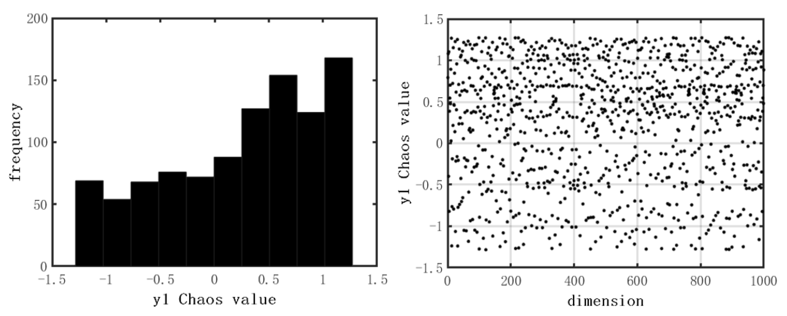
3.3.1. Hénon Chaotic Mapping

Since the sparrow population is randomly generated during the initialization of the population by the original SSA algorithm, this leads to a lack of diversity in the sparrow population, which in turn leads to a decrease in the global search ability of the algorithm and a poor convergence rate. The chaotic phenomenon refers to the existence of some irregular variables in a definite system, and these variables are not repeatable, unpredictable, or uncertain. Given the stochastic nature of chaotic variables, they can be used to increase the population diversity of the original SSA algorithm and enhance the algorithm’s ability to leapfrog local optima and global searches.

In this paper, Hénon chaotic mapping is used to initialize the population of the SSA algorithm, as shown in Formula (8):

$$\left\{\begin{array}{c}{y}_1\left(t\right)=1-a\left(y_1\right(t-1){)}^2+y_2(t-1)\\ y_2\left(t\right)=b{y}_1\left(t\right)\end{array}\right. ,$$

(8)

where t represents the number of chaotic iterations. The research results show that when $a$ = 1.4 and b = 0.3, the function enters the chaotic state, and the generated chaotic sequence has strong randomness [33]. Figure 3 shows the distribution histogram and evolutionary scatter plot of the values of the Hénon chaotic sequence.

In this paper, the Hénon chaotic sequence $y_1\left(t\right)$ is used to regulate it from the range [−1.28, 1.27] to [0, 1] according to Formula (9).

$$z\left(t\right)=\mathit{abs}\left(\omega y_1\left(t\right)\right),t=\mathrm{1,2},\cdots ,n.$$

(9)

Finally, the position of the initial sparrow is obtained through Formula (10).

$$x_i^t=l{b}_i+z\left(t\right)\left(u{b}_i-l{b}_i\right),$$

(10)

where $u{b}_i$ and $l{b}_i$ are the upper and lower bounds in the corresponding solution space, respectively.

3.3.2. Multidirectional Learning Strategies

In the SSA algorithm, each follower selects only one finder with a higher fitness value than itself to learn from at a time, without considering the information from other individuals. Although this random learning approach facilitates the exploration of the search space, it significantly reduces the population’s diversity. Consequently, there is a higher likelihood of the algorithm getting trapped in local extremum regions, ultimately limiting its ability to find the global optimum. To provide disadvantaged sparrow individuals with more opportunities to explore areas that may go unnoticed by the population within the search space, we employ multidirectional learning strategies to enhance follower positions. The updated formula is as follows:

$$X_{i,j}^{t+1}=\left\{\begin{array}{c}\hspace{1em}Q·\exp \left(\frac{X_{\mathrm{worst}}-X_{i,j}^t}{i^2}\right),i>\frac{n}{2}\\ \frac{{\tau }_a·X_{a,j}^t+{\tau }_b·X_{b,j}^t+{\tau }_c·X_{c,j}^t}{{\tau }_a+{\tau }_b+{\tau }_c},i\le \frac{n}{2}\end{array}\right.,$$

(11)

where ${\tau }_a$, ${\tau }_b$, and ${\tau }_c$ denote the weights of individual sparrows at points a, b, and c, respectively, and the specific expression is:

$$\left\{\begin{array}{c}\begin{array}{c}{\tau }_a=\frac{f_a+f_b+f_c}{f_a}\\ {\tau }_b=\frac{f_a+f_b+f_c}{f_b}\\ {\tau }_c=\frac{f_a+f_b+f_c}{f_c}\end{array}\end{array}\right.,$$

(12)

where $f_a$, $f_b$, and $f_c$ denote the fitness values of the sparrows located at points a, b, and c, respectively. The weights assigned to the three sparrows are calculated based on the fitness values, so that the sparrow with the better fitness value has a greater weight. The follower at this point synthesizes the positional information of the other three sparrows to detect undetected areas of the current search space with greater probability, further improving the population’s ability to explore the search space.

3.3.3. Crossover and Mutation

The iterative process of the SSA algorithm is a process of constantly approaching the optimal individual. If the current optimal individual is a local optimal individual, the SSA algorithm is very prone to local optimal stagnation. In this paper, crossover and mutation operations are performed on the optimal values of the finder population with a certain probability. The crossover probability (pc) is a critical parameter that influences the balance between operator exploitation and exploration. Commonly used probabilities are fixed values, but setting them too high can increase the randomness of the population after crossover, disrupt the population’s balance, and result in the algorithm’s inability to converge. Conversely, setting them too low can affect the convergence capability of the population and slow down the evolutionary speed of the population. Therefore, this article adopts an adaptive adjustment of the pc value, as shown in Formula (13).

$$pc=p{c}_{min}+\left(p{c}_{max}-p{c}_{min}\right)\times \frac{1}{1+\mathit{exp}\left(\frac{{f^{\prime }}_{min}^{ }-f_{avg}}{{f^{\prime }}_{max}^{ }-f_{avg}}\right)},$$

(13)

where $p{c}_{min}$ and $p{c}_{\mathrm{m}\mathrm{a}\mathrm{x}}$ are the minimum and maximum probabilities of crossover; $f_{avg}$ is the average fitness value of the population in each generation; and ${f\prime }_{\mathrm{m}\mathrm{a}\mathrm{x}}^{}$ and ${f\prime }_{\mathrm{m}\mathrm{i}\mathrm{n}}^{}$ are the individuals with the largest and smallest fitness values in the two populations to be crossover, respectively.

Randomly select an individual from the finder population and, with a certain mutation probability (pm), make a random change in the structural data of the selected individual. The mutation probability (pm) is a critical parameter that affects the solution quality and convergence of the operator. A too large pm can lead to significant changes in the evolutionary direction of the population, which is detrimental to convergence, while a too small pm can result in the insufficient generation of new individuals, leading to a lack of diversity in the population. This paper adopts an adaptive adjustment of pm, as shown in Formula (14).

$$pm=\left\{\begin{array}{c}p{m}_{\mathrm{m}\mathrm{a}\mathrm{x}}-\left(p{m}_{\mathrm{m}\mathrm{a}\mathrm{x}}-p{m}_{\mathrm{m}\mathrm{i}\mathrm{n}}\right)\times \frac{f-f_{\mathrm{a}\mathrm{v}\mathrm{g}}}{f_{\mathrm{m}\mathrm{a}\mathrm{x}}-f_{\mathrm{a}\mathrm{v}\mathrm{g}}},f>p{m}_{\mathrm{a}\mathrm{v}\mathrm{g}}\hfill \\ p{m}_{\mathrm{m}\mathrm{a}\mathrm{x}} , f\le p{m}_{\mathrm{a}\mathrm{v}\mathrm{g}}\end{array}\right.,$$

(14)

where $f_{\mathrm{m}\mathrm{a}\mathrm{x}}$ and $f_{\mathrm{a}\mathrm{v}\mathrm{g}}$ are the maximum individual fitness and average fitness of the population, respectively; $f$ is the current individual fitness of the population; and $p{m}_{\mathrm{m}\mathrm{i}\mathrm{n}}$ and $p{m}_{\mathrm{m}\mathrm{a}\mathrm{x}}$ are the minimum and maximum probability of variation, respectively. Mutation is the process by which a new species randomly generates new genes to increase the abundance of a genetic population.

3.4. ISSA-BP Neural Network Approach for SST Retrieval

The improved SSA algorithm is used to optimize the BP neural network, and then the ISSA-BP model is obtained. The basic idea is to take the initial weights and thresholds of the BP neural network algorithm as the optimization target of the SSA algorithm and the mean squared error in the prediction algorithm as the adaptation value of the SSA algorithm. After several iterations, the results are assigned to the BP neural network algorithm to enhance its optimization ability and improve the retrieval SST accuracy of the ISSA-BP model. The preprocessed 14,252 datasets were divided into training and test sets in a 7:3 ratio. The dual-polarized (vertically and horizontally polarized) brightness temperature data from AMSR2 satellites at 6.9, 7.3, 10.7, 18.7, 23.8, 36.5, and 89.0 GHz, sea surface winds, and latitude/longitude information at the matched positions serve as the input elements. The output element is the SST derived from the ARGO buoy-measured data. The SST retrieval flow is shown in Figure 4.

3.4.1. Neural Network Algorithm Initialization

There are two general types of parameters in a machine learning model: parameters used during training and hyperparameters assigned prior to training. Hyperparameters can be tuned to improve model performance. To determine the specific values of hyperparameters in BP neural networks, we used the GridSearchCV method of cross-validation provided by the sklearn library in Python [34]. Grid search is a common method for parameter tuning in machine learning, and its primary purpose is to explore different combinations of hyperparameters to optimize the model. Based on the grid search results, we determined the following hyperparameter values: 15 neurons in the hidden layer, 1000 iterations, and the ReLU activation function.

The Sigmoid function and Tanh function, which are commonly used in BP neural networks as activation functions, are prone to situations where the derivative tends to 0. This can make gradient descent slower and is not conducive to the propagation of gradients in the network. Instead, the model uses the ReLU function as the activation function expression: $f\left(x\right)=\mathrm{m}\mathrm{a}\mathrm{x}(0, x)$. The ReLU function’s local gradient is never 0, which is beneficial for the propagation of gradient flow. Furthermore, it does not have a saturation region, to some extent resisting the vanishing gradient problem to ensure training speed. The model employs an Adam optimizer to further improve training efficiency. The Adam optimizer corrects the first-order moment and second-order moment estimates, which are initialized from the origin. Compared to the RMSProp algorithm, it also corrects bias to ensure a dynamically adjusted range of learning rates at each iteration. In this experiment, the initial learning rate is set to 0.01, and when the error loss in the test set decreases slowly, the learning rate decays by a factor of (1/2)n, so that it is finally reduced to 0.00125. In order to prevent the overfitting problem due to the small number of training samples, in this study, with the help of the Dropout algorithm [35], the neurons are randomly deactivated with a certain probability, and the experimental selection is 0.5. The specific parameters of the experiment are shown in

Table 2. Neural network parameter settings.

Parameters	Model Settings	Parameters	Model Settings
Number of input layers	17	Dropout location	Between the hidden layer and the activation function
Number of output layers	1	Dropout loss ratio	0.5
Number of hidden layers	15	Learning rate	0.1 attenuation to 0.00125
Activation function	ReLU	Number of iterations	1000
Optimizer	Adam	Number of batch processes	50

.

3.4.2. SSA Parameter Initialization

Using the whole population to represent the initial weights and thresholds in the BP neural network, the initial coding length can be obtained based on the number of neurons in the input, hidden, and output layers. The calculation is shown in Formula (15), and the final optimized number of population dimensions, dim = 286, is obtained.

$$dim=n\times h+h\times m+h+m,$$

(15)

where n is the number of neurons in the input layer in the BP neural network algorithm; h is the number of neurons in the hidden layer in the BP neural network algorithm; and m is the number of neurons in the output layer in the BP neural network algorithm.

In the experiment, the initial sparrow population size was 50; the maximum number of iterations was 30; the upper- and lower-boundary values for thresholds and weights were 5 and −5, respectively; the proportion of finders in the population was 0.2; the proportion of vigilantes was 0.1; and the safety threshold ST was 0.6.

The mean squared error (MSE) is the average of the sum of the squares of the deviations of the sample data from the true values. In other words, it represents the average of the sum of the squared errors. It can measure the relationship between the sample data and the true value; the smaller the MSE value, the higher the accuracy of the prediction algorithm, and the higher the fit between the predicted value and the true value. Therefore, the mean squared error is used as the individual fitness value of the SSA algorithm, and its calculation formula is shown in Formula (16).

$$MSE=\frac{1}{n}\sum _{i=1}^n(c_i-y_i{)}^2,$$

(16)

where n is the number of samples, $c_i$ is the predicted value, and $y_i$ is the actual value.

4. Experiments and Results

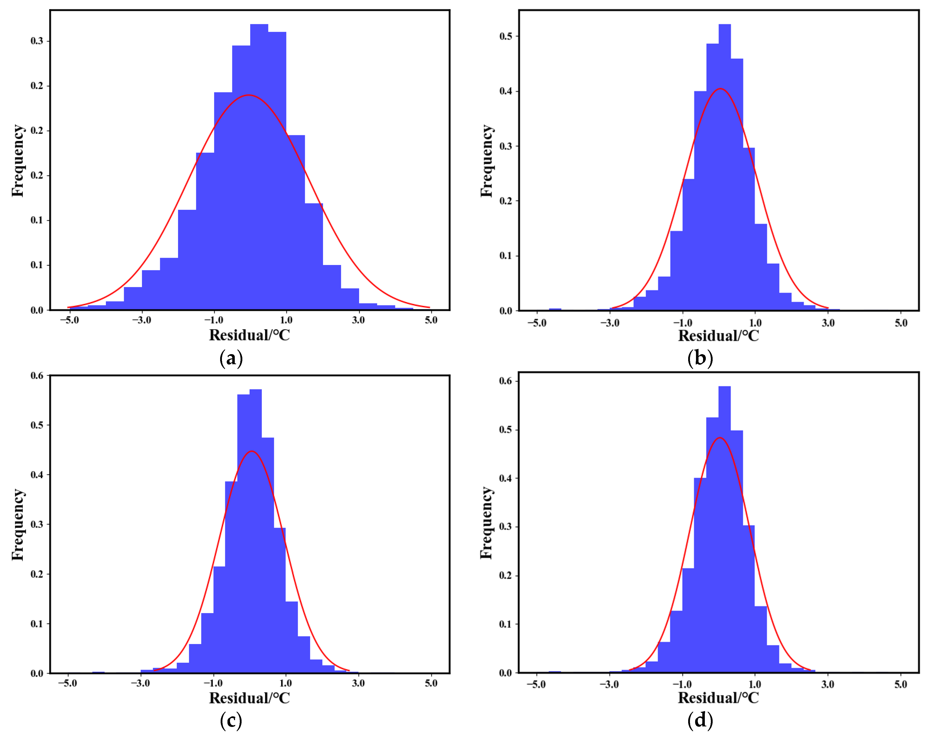
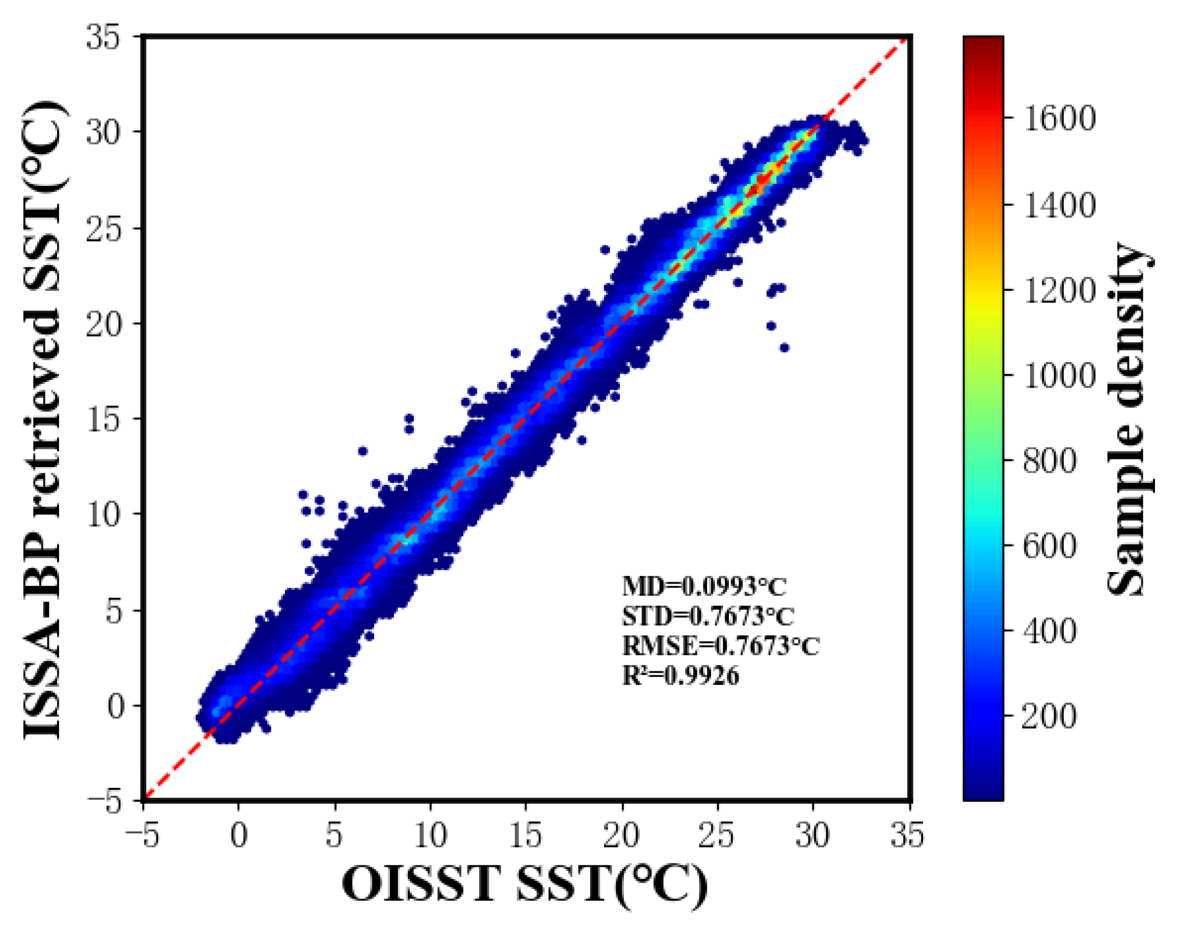
4.1. Comparing Multiple Models to Retrieve SST with In Situ SST

Based on the test set of matched datasets, a multiple linear regression (MLR) model was constructed as a benchmark for comparing the performance of the ISSA-BP model. The MLR algorithm is a common operational retrieval algorithm for satellite-borne microwave radiometers that inverts the sea–air covariates using linear combinations or disguised linear combinations of the observed brightness temperature values of multiple channels of the microwave radiometer. The algorithm is summarized as:

$$\mathrm{S}\mathrm{S}\mathrm{T}=a_0+\sum _{i=1}^n a_i\times T_{Bi} ,$$

(17)

where $a_0$ and $a_i$ are the fitting coefficients, $T_{Bi}$ is the value of the brightness temperatures of a certain channel, and n is the number of channels. This method assumes a certain linear relationship between ocean parameters such as sea surface temperature, sea surface wind speed, and the brightness temperatures observed by each channel of the radiometer, and a set or groups of coefficients are obtained by statistically regressing the time-matched starboard radiometer measurements on the buoy data and the reanalyzed data for the retrieval of ocean parameters.

In addition, in order to evaluate the performance of the ISSA-BP neural network model constructed in this paper more comprehensively, the algorithm in this paper is also compared with the base BP neural network and the BP neural network model optimized by the unimproved SSA algorithm (SSA-BP) on test set data. Four indexes (the root-mean-square error (RMSE), the mean absolute error (MAE), the mean absolute percentage error (MAPE), and the R²) are used for evaluation. The formulas are as follows, and the results are shown in

Table 3. Overall performance of the four algorithms.

Error Assessment Indicators	Retrieval Model
	MLR	BP	SSA-BP	ISSA-BP
RMSE (°C)	1.6674	0.9882	0.8952	0.8268
MAE (°C)	1.1103	0.6623	0.6010	0.5801
MAPE (%)	30.2298	20.0492	18.7003	15.1603
R2	0.9647	0.9882	0.9903	0.9918

.

$$RMSE=\sqrt{\frac{1}{n}\sum _{i=1}^n (X_i-Y_i{)}^2},$$

(18)

$$\mathit{MAE}=\frac{1}{n}\sum _{i=1}^n |X_i-Y_i|,$$

(19)

$$\mathit{MAPE}=\frac{1}{n}\sum _{i=1}^n \frac{ |X_i-Y_i| }{X_i} ,$$

(20)

$$R^2=1-\frac{\sum _{i=1}^n (Y_i-X_i{)}^2}{\sum _{i=1}^n (X_i-\overline{X_i}{)}^2} ,$$

(21)

where n is the number of samples, $Y_i$ is the predicted value, and $X_i$ is the actual value.

As can be seen from Table 3, the ISSA-BP neural network model constructed in this paper outperforms other models in all the evaluation indexes, proving the effectiveness of the ISSA-BP neural network model in retrieving sea surface temperature.

(1)

ISSA-BP model compared to the MLR model: the RMSE decreased by 50.41%, the MAE decreased by 47.75%, the MAPE decreased by 49.85%, and the R² increased by 2.81%.

(2)

ISSA-BP model compared to the base BP neural network model: the RMSE decreased by 16.33%, the MAE decreased by 12.41%, the MAPE decreased by 24.38%, and the R² increased by 0.36%.

(3)

ISSA-BP model compared to the SSA-BP model: the RMSE decreased by 7.64%, the MAE decreased by 3.48%, the MAPE decreased by 8.93%, and the R² increased by 0.15%.

In order to visualize the deviation of the retrieved SST value from the measured value for each checkpoint, for each algorithm, the measured SST value is used as the horizontal vertical axis of the planar right-angled coordinate system, and the retrieved SST value is used as the vertical axis, and all the checkpoints are plotted in this coordinate system. The deviation of the retrieved values from the measured values for the various algorithms is obtained, as shown in Figure 5. Most of the scatter points of the four models are near the reference line. The figure shows that the ISSA-BP neural network model has the least number of anomalous scatter points and the best retrieval results.

Figure 6a–d show the histograms of the residual distribution of the multiple linear regression, BP neural network, SSA-BP neural network, and ISSA-BP neural network models, respectively. The overall trend of the four plots conforms to the normal distribution, with more data in the intervals of smaller residual values and a significant decrease in the range of intervals of larger residual values on both sides. Most of the retrieval errors in the ISSA-BP neural network model are concentrated in the range of small errors with the highest accuracy.

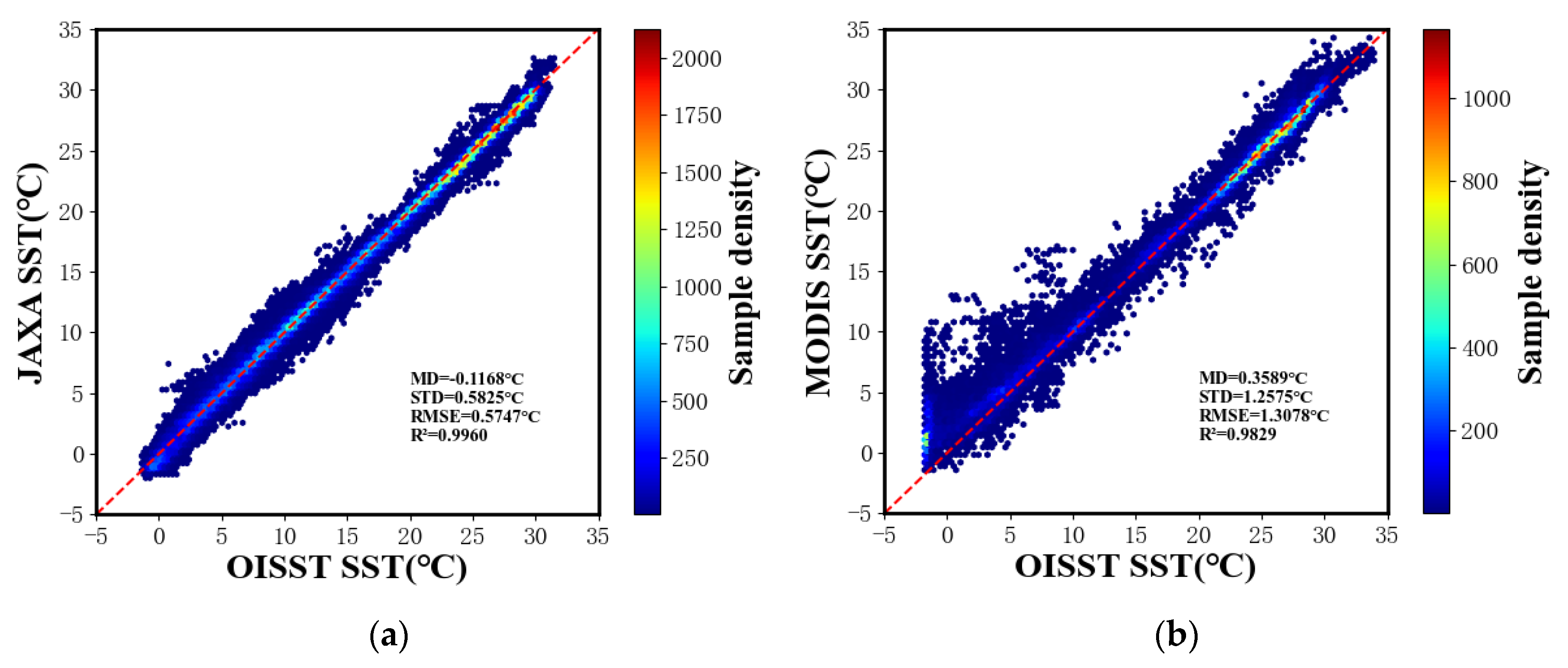
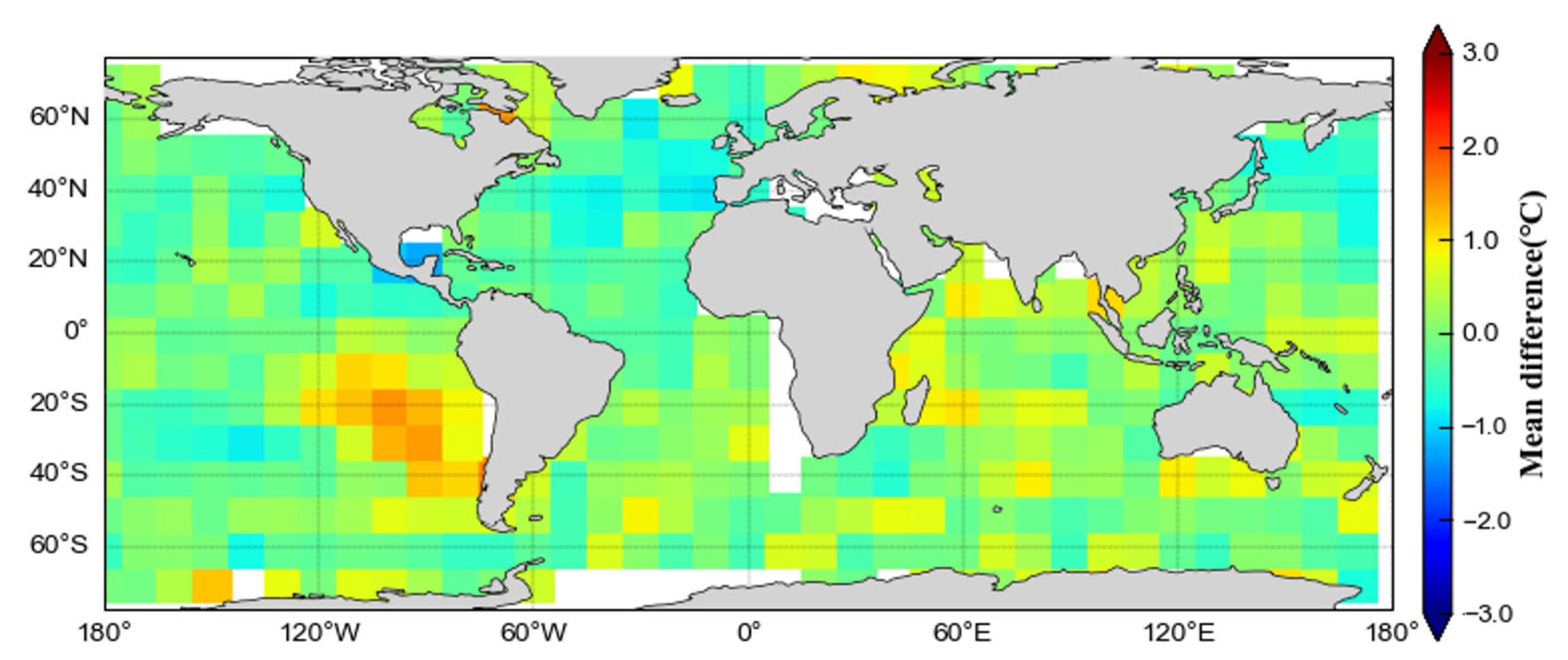
4.2. Comparison of ISSA-BP Model Retrieval Results with Multiple SST Products

Global SSTs were retrieved, and spatial distribution maps were generated by inputting into the ISSA-BP retrieval model (Figure 7) JAXA AMSR2 Level-3 descending orbit brightness temperature data at a 0.25° spatial resolution on 15 July 2022 and AMSR2 Level-3 sea surface wind speed data at a 0.25° resolution on the same date. The retrieved SSTs were compared with the optimum interpolation sea surface temperature (daily OISST) for the same date (Figure 8), and the results are presented in Figure 9. The 0.25° daily OISST is an analysis constructed by blending measurements from different platforms (satellites, ships, buoys) on a regular global grid. A spatially complete global map of SST is produced by interpolation to fill gaps, offering the advantages of timeliness and global coverage [36]. The coefficient of determination of OISST versus SST retrieved by the ISSA-BP model was 0.9926, with a root-mean-square error of 0.7673 °C.

To further validate the retrieval effectiveness of the resulting model, we compared the JAXA AMSR2 Level-3 SST standard product (Figure 10) and the MODIS Aqua Level-3 SST product (Figure 11) with the OISST, respectively. Since the spatial resolution of MODIS SST data is 4 km and the spatial resolution of the OISST is 0.25° × 0.25°, we employed mean spatial aggregation of MODIS SST data for dimensionality reduction. Please refer to Figure 12 for the comparison results. The mean deviations of the JAXA SST and the MODIS SST compared with the OISST are −0.1168 °C and 0.3589 °C, with root-mean-square errors of 0.5747 °C and 1.3078 °C, respectively. Using the OISST as the reference benchmark, the SST accuracy retrieved by the model in this paper is much higher than that of the MODIS SST and comparable to that of the JAXA SST product.

Since the SST retrieved by the ISSA-BP model has the same resolution as the OISST, which is 0.25° × 0.25°, the values at the corresponding grid points were selected. The SST obtained from the retrieval was then used to subtract the OISST. The results were calculated on a spatial grid of 10° × 10° in terms of the mean deviation (Figure 13) and the standard deviation of the error (Figure 14). It can be clearly seen that the global regional mean deviations are concentrated in a smaller range, mostly within 2 °C. The geographical distribution of the error standard deviation is clearly related to latitude.

5. Discussion

In this paper, we chose the BPNN as the fundamental model for SST retrieval because it can extract “rules” between input features and output objects through learning and store this knowledge in network weights, demonstrating high self-learning and self-adaptability. However, as the scope of its application expands, the BPNN algorithm has revealed several shortcomings. When the number of training sets remains constant, the main factors influencing prediction accuracy are the two parameters of BPNN initialization: weights and thresholds. Typically, these parameters are randomly generated within a fixed range, and the selection of initial weights can significantly impact the prevention of local minima and the convergence speed of the network. Improperly selected parameters, such as weights and thresholds, can hinder network convergence. To address this issue, we optimized the weight and threshold parameters using an Improved Sparrow Search Algorithm (ISSA). This algorithm retains the advantages of the original version while incorporating enhancements. Firstly, during the initialization stage, we improved the quality of the initial solution by introducing the Hénon chaos strategy. Secondly, we employed a multidirectional learning strategy to enhance the exploration capabilities of the sparrow and its followers across the entire search space. Finally, we invoked the mutation operator from genetic algorithms to transform locally optimal solutions into new solutions. As a result, we obtained the ISSA-BP SST retrieval model.

The model was tested and analyzed using the test dataset reserved from the matched datasets. The coefficient of determination (R²) between the SST retrieved by the ISSA-BP model and the measured data from the ARGO buoys is 0.9918, and the root-mean-square error (RMSE) is 0.8268 °C. Several scholars have previously employed the NN approach for SST retrieval. Lei Meng et al. [15] utilized SSM/I observations of brightness temperature to retrieve SST using an NN, with an RMSE of 1.54 °C between the retrieved and measured values of SST. Biao Zhang et al. [37] used the 12 frequency channels of AMSR2’s brightness temperature (6.9–36.5 GHz) to simultaneously retrieve sea surface wind speed, SST, near-surface air temperature, and dewpoint temperature based on a BPNN model. The RMSE of the retrieved SSTs compared with the NDBC and TAO buoy measurements is 1.02 °C. Wang et al. [38] applied a radial basis function neural network (RBFNN) method to retrieve SST in global coastal waters using PMW radiometer measurements. The model retrieved global coastal sea SST with an average deviation of 0.071 °C and an RMSE of 1.18 °C. Ai Bo et al. [39] proposed an infrared remote sensing retrieval model of SST based on a deep NN using moderate-resolution imaging spectroradiometer (MODIS) infrared remote sensing data in Bohai. The standard error was 0.71 °C, and the mean absolute deviation was 0.85 °C. Zheng et al. [40] used the artificial neural network (ANN) integration (ANNE) method to construct the scanning microwave radiometer SST retrieval algorithm. The RMSE of the ANNE algorithm compared with the global iQuam SSTs is 1.46 °C. According to the results in Figure 5d, there is a good correlation between the ISSA-BP retrieval results and the buoy-measured data with an excellent fit. The ISSA-BP model also demonstrates excellent accuracy compared with the results of previous studies using NN methods to retrieve SST, indicating that the established method model is suitable for retrieving global sea surface temperature. The multiple linear regression model achieved a coefficient of determination R² of 0.9647 and an RMSE of 1.6673 °C, which represents the lowest accuracy among all models. This illustrates the superiority of the machine learning method over the traditional statistical regression approach. In Figure 6d, the residual distribution of the ISSA-BP model is concentrated in the range of less than 1 °C compared with other models, and the amount of data within this error range decreases almost exponentially as the retrieval error increases, so the overall error of the SSTs retrieved by using the model in this paper is on the small side. Due to its more powerful nonlinear regression prediction ability, the ISSA-BP model exhibits better retrieval accuracy compared to the traditional model.

Overall, most of the sea surface temperature retrievals from all models are larger than the “true value” when the sea surface temperature is low (<5 °C). This is consistent with the conclusion of Gentemann and Hilburn [41] that bias and uncertainty increase at lower temperatures when retrieving sea surface temperatures with AMSR2. This phenomenon may result from the fact that the sensitivity of brightness temperatures to sea surface temperature decreases in cold water, as suggested by previous studies [42,43]. The best retrieval results were obtained when the sea surface temperature was in the range of 5–20 °C. At higher sea surface temperatures (>25 °C), most of the sea surface temperature retrieval results from all models were basically consistent with the measured values, except for the multiple linear regression model, which had more discrete points. The difference between the sea surface temperatures retrieved by the ISSA-BP model and the buoy observations may be related to several factors. First, AMSR2 retrieves sea surface temperatures based on averages over its resolution cells, whereas the buoys provide temporal averages over a single localization point. Therefore, there is an unavoidable error in matching the AMSR2 brightness temperature data with the buoy observations. Secondly, AMSR2 senses the surface temperature of the ocean (to a depth of a few millimeters), whereas the ARGO buoys measure the temperature of the seawater at a depth of 0.2–1.5 m, and the phenomenon of daily warming of the seawater can cause the temperature difference between this surface and the surface during the daytime. Finally, the AMSR2 brightness temperatures can be contaminated by RFI, which in turn affects the accuracy of sea surface temperature retrieval. Although in this study we use the 6.9 and 10.7 GHz channel brightness temperatures to eliminate RFI contamination, this effect cannot be eliminated by this operation.

Retrieving global sea surface temperatures on 15 July 2022, according to the ISSA-BP model, the coefficient of determination between the retrieved SST and the OISST reaches 0.9926, with a deviation of 0.0993 °C and a root-mean-square error of 0.7673 °C. Using the OISST as a reference, the SST retrieved by the model in this paper is significantly more effective than the MODIS SST. The root-mean-square error of the SST retrieved by the model in this paper is comparable to that of the JAXA SST in terms of “release accuracy” (0.8 °C), but higher than that of “standard accuracy” (0.5 °C) [37]. We believe that this may be related to the amount of data used to train the model. If there is insufficient training data for a specific range of SSTs, such as very cold and hot SSTs, it will be challenging for the ML model to learn how to retrieve these SSTs. Therefore, the uneven distribution of the training data might explain part of the retrieval error. Training separate instances of the ML models for very cold and very warm SSTs might result in better performance. The trend of the global SST distribution retrieved from the ISSA-BP model is reasonable, and the retrieval results are basically consistent with the actual situation, with the high-value areas concentrated in the middle and low latitudes, while the low-value areas are distributed in the high latitudes. The characteristics of oceanic fronts in the region of the Japanese Warm Current and the Gulf Stream are also clearly shown in Figure 7, with a temperature difference of about 8 °C on both sides of the fronts. Higher sea surface temperatures (28–31 °C) are found in the north-west Pacific, North Indian Ocean, north-east Pacific, and equatorial regions. Lower sea surface temperatures (15–20 °C) are found in two equatorial subregions, including the southeastern Atlantic Ocean and the southeastern Pacific Ocean. This phenomenon may be attributed to the presence of cold currents, specifically the Peru and Benguela currents, which transport cold water from the South Pacific and the South Atlantic Ocean to these subregions, consequently leading to lower sea surface temperatures. In addition, two sub-Arctic currents (the Thousand Islands Current and the Labrador Current) transport cold water from the Arctic Ocean to Japan and northeastern Newfoundland, resulting in cooler sea surface temperatures (about 5–10 °C).

According to the results of Figure 13, at high latitudes, especially in the Southern Ocean, there are large positive deviations, which, near the poles, are confirmed to be related to the effects of sea ice [16]. It is also believed that the effect of sea surface winds may play a role in the large deviations. Since the Southern Ocean is characterized by very high wind speeds, the results of the retrieval may be affected [44]. Large negative biases can be seen in the tropical western Pacific, Mexico regions, and the Arabian Sea, all of which are characterized by higher temperatures. This suggests that the ISSA-BP model has a cold bias towards SSTs with high temperatures. According to the results of Figure 14, the geographical distribution of the error standard deviation shows an obvious relationship with latitude, exhibiting a higher standard deviation in high-latitude regions and a lower standard deviation in low-latitude regions. The lowest standard deviation bias occurs between 40° north and south latitudes, and the standard deviation tends to increase with higher latitudes. The PMW SST validation results of Alerskans et al. [20] and Nielsen-Englyst et al. [22] both show the same latitudinal dependence as shown in Figure 14. Gentemann reported similar results [45], with the lowest standard deviation between 40°S and 40°N and higher values for increasing latitude. The larger standard deviations near the poles can be attributed to the presence of sea ice, which can contaminate microwave observations, as well as the fact that brightness temperature is less sensitive to SST at colder temperatures than at warmer temperatures [46]. In this paper, the ISSA-BP model retrieves SSTs with an increased bias and standard deviation for very warm and very cold regions. It is well known that machine learning models often face challenges in predicting extreme values [47]. In NN algorithms, optimization is performed based on the minimization of a loss function. Since this loss function measures the average performance of the model over a range of target variables, the richest cases have the greatest impact on the model’s performance. The effect of rare cases is almost negligible, so the model’s performance in these cases may suffer. Consequently, it is difficult for machine learning models to accurately retrieve SSTs from very cold and very hot cases due to a lack of sufficient training data for these extremes.

Sea surface temperature retrieval is a complex problem that has caused extensive and in-depth research from all walks of life. Machine learning is currently at the peak of vigorous development and has a wide range of applications in various fields of research. The fitting effect of the BPNN for modeling the nonlinear relationships among multiple variables is not always optimal, particularly in complex problems with large datasets. Previous studies have shown that deep learning [48] algorithms have strong modeling and generalization capabilities in regression prediction problems and are especially suitable for processing large-scale, complex, and nonlinear data. However, they also require a substantial amount of data and computing resources and may not perform as well as traditional machine learning methods on some small datasets or with limited resources. Exploring different methods for achieving high-precision sea surface temperature retrieval is a research problem that warrants further investigation.

6. Conclusions

Based on research involving the Back-Propagation neural network (BPNN) and the Sparrow Search Algorithm (SSA), a new method for retrieving sea surface temperature (SST) using passive microwave measurements is proposed. Addressing the issue that an improper selection of weights and thresholds in the BPNN model may adversely affect the results, the parameters of weights and thresholds are optimized using the Improved Sparrow Search Algorithm, resulting in the ISSA-BP model. The ISSA-BP combines the advantages of both physical process-based and statistical methods, providing a strong ability to handle nonlinear problems and good fault tolerance. Additionally, it avoids the complexities associated with using radiative transfer models, making it an effective method for sea surface temperature retrieval. This study represents a preliminary exploration into the use of machine learning methods for the simple and efficient retrieval of sea surface temperature from passive microwave observations. The comparison and analysis of the retrieval results of the ISSA-BP model with the buoy-measured data show that the model has higher accuracy results. Its retrieval effect is significantly better than that of the traditional multiple linear regression method, the basic BPNN model, and the BPNN optimized by the unimproved Sparrow Search Algorithm. Meanwhile, the model-retrieved results are cross-validated with OISST products and found to be in good agreement. It also demonstrates good accuracy compared to the MODIS SST product and the JAXA SST product. The experimental results illustrate that the established methodology model is suitable for retrieving SST, indicating significant potential for using machine learning models in sea surface parameter retrieval. This study can serve as a reference for subsequent research. By incorporating more in situ observations from the global ocean into the training dataset and considering other parameters that affect SST or satellite brightness temperature as additional input elements, we believe the existing BPNN model can be further improved.

References

1. Kawai, Y.; Wada, A. Diurnal sea surface temperature variation and its impact on the atmosphere and ocean: A review. J. Oceanogr. 2007, 63, 721–744. [Google Scholar] [CrossRef]
2. Chelton, D.B.; Wentz, F.J. Global microwave satellite observations of sea surface temperature for numerical weather prediction and climate research. Bull. Am. Meteorol. Soc. 2005, 86, 1097–1116. [Google Scholar] [CrossRef]
3. Kent, E.C.; Kennedy, J.J.; Smith, T.M.; Hirahara, S.; Huang, B.; Kaplan, A.; Parker, D.E.; Atkinson, C.P.; Berry, D.I.; Carella, G. A call for new approaches to quantifying biases in observations of sea surface temperature. Bull. Am. Meteorol. Soc. 2017, 98, 1601–1616. [Google Scholar] [CrossRef]
4. Hu, X.; Zhang, C.; Shang, S. Validation and inter-comparison of multi-satellite merged sea surface temperature products in the South China Sea and its adjacent waters. J. Remote Sens. 2015, 19, 328–338. [Google Scholar]
5. Sun, L.; Wang, J.; Cui, Y.; Hao, Y.; Zhang, J. Statistical retrieval algorithms of the sea surface temperature (SST) and wind speed (SSW) for FY-3B Microwave Radiometer Imager (MWRI). J. Remote Sens. 2012, 16, 1262–1271. [Google Scholar]
6. Wang, Y.; Fu, Y.; Liu, Q.; Liu, G.; Liu, X.; Cheng, J. An algorithm for sea surface temperature retrieval based on TMI measurements. Acta Meteorol. Sin. 2011, 69, 149–160. [Google Scholar]
7. Milman, A.; Wilheit, T. Sea surface temperatures from the scanning multichannel microwave radiometer on Nimbus 7. J. Geophys. Res. Oceans 1985, 90, 11631–11641. [Google Scholar] [CrossRef]
8. Wentz, F.J.; Gentemann, C.; Smith, D.; Chelton, D. Satellite measurements of sea surface temperature through clouds. Science 2000, 288, 847–850. [Google Scholar] [CrossRef]
9. Han, Z.; Huo, W.; Wang, S. Retrieval of sea surface temperature from AMSR-E and MODIS in the northern Indian ocean. In Proceedings of the 2012 2nd International Conference on Remote Sensing, Environment and Transportation Engineering, Nanjing, China, 1–3 June 2012; pp. 1–4. [Google Scholar]
10. Shibata, A. Improvement of AMSR-E SST by considering an elaborate correction of wind effect. In Proceedings of the 2005 IEEE International Geoscience and Remote Sensing Symposium (IGARSS’05), Seoul, Republic of Korea, 29 July 2005; pp. 2612–2613. [Google Scholar]
11. Wang, Z.; Li, Y. Retrieval of marine geophysical parameters using spaceborne microwave radiometer AMSR-E data. J. Remote Sens. 2009, 13, 363–370. [Google Scholar] [CrossRef]
12. Krasnopolsky, V.M. Neural network emulations for complex multidimensional geophysical mappings: Applications of neural network techniques to atmospheric and oceanic satellite retrievals and numerical modeling. Rev. Geophys. 2007, 45, 3. [Google Scholar] [CrossRef]
13. Krasnopolsky, V.; Breaker, L.; Gemmill, W. A neural network as a nonlinear transfer function model for retrieving surface wind speeds from the special sensor microwave imager. J. Geophys. Res. Oceans 1995, 100, 11033–11045. [Google Scholar] [CrossRef]
14. Krasnopolsky, V.M.; Gemmill, W.H.; Breaker, L.C. A neural network multiparameter algorithm for SSM/I ocean retrievals: Comparisons and validations. Remote Sens. Environ. 2000, 73, 133–142. [Google Scholar] [CrossRef]
15. Meng, L.; He, Y.; Chen, J.; Wu, Y. Neural network retrieval of ocean surface parameters from SSM/I data. Mon. Weather Rev. 2007, 135, 586–597. [Google Scholar] [CrossRef]
16. Alerskans, E.; Zinck, A.-S.P.; Nielsen-Englyst, P.; Høyer, J.L. Exploring machine learning techniques to retrieve sea surface temperatures from passive microwave measurements. Remote Sens. Environ. 2022, 281, 113–220. [Google Scholar] [CrossRef]
17. Qi, G.; Wei, D. Prediction of hydroelectric engineering cost index based on GA-BP neural network. Water Resour. Power 2018, 36, 162–164. [Google Scholar]
18. Shi, L.; Ding, X.; Li, M.; Liu, Y. Research on the capability maturity evaluation of intelligent manufacturing based on firefly algorithm, sparrow search algorithm, and BP neural network. Complexity 2021, 2021, 5554215. [Google Scholar] [CrossRef]
19. Xue, J.; Shen, B. A novel swarm intelligence optimization approach: Sparrow search algorithm. Syst. Sci. Control Eng. 2020, 8, 22–34. [Google Scholar] [CrossRef]
20. Alerskans, E.; Høyer, J.L.; Gentemann, C.L.; Pedersen, L.T.; Nielsen-Englyst, P.; Donlon, C. Construction of a climate data record of sea surface temperature from passive microwave measurements. Remote Sens. Environ. 2020, 236, 111–485. [Google Scholar] [CrossRef]
21. Block, T.; Embacher, S.; Merchant, C.J.; Donlon, C. High-performance software framework for the calculation of satellite-to-satellite data matchups (MMS version 1.2). Geosci. Model Dev. 2018, 11, 2419–2427. [Google Scholar] [CrossRef]
22. Nielsen-Englyst, P.; Høyer, J.L.; Toudal Pedersen, L.; Gentemann, C.L.; Alerskans, E.; Block, T.; Donlon, C. Optimal estimation of sea surface temperature from AMSR-E. Remote Sens. 2018, 10, 229. [Google Scholar] [CrossRef]
23. Imaoka, K.; Maeda, T.; Kachi, M.; Kasahara, M.; Ito, N.; Nakagawa, K. Status of AMSR2 instrument on GCOM-W1. In Proceedings of the Earth Observing Missions and Sensors: Development, Implementation, and Characterization II, Kyoto, Japan, 30 October–1 November 2012; pp. 201–206. [Google Scholar]
24. Hihara, T.; Kubota, M.; Okuro, A. Evaluation of sea surface temperature and wind speed observed by GCOM-W1/AMSR2 using in situ data and global products. Remote Sens. Environ. 2015, 164, 170–178. [Google Scholar] [CrossRef]
25. Alsweiss, S.O.; Jelenak, Z.; Chang, P.S. Remote sensing of sea surface temperature using AMSR-2 measurements. IEEE J. Sel. Top. Appl. Earth Obs. Remote Sens. 2017, 10, 3948–3954. [Google Scholar] [CrossRef]
26. Pearson, K.; Merchant, C.; Embury, O.; Donlon, C. The role of advanced microwave scanning radiometer 2 channels within an optimal estimation scheme for sea surface temperature. Remote Sens. 2018, 10, 90. [Google Scholar] [CrossRef]
27. Argo Data Management Team. Argo User’s Manual v3.3; Argo Data Management Team: Brest, France, 2019. [Google Scholar]
28. Dee, D.; Uppala, S.; Simmons, A.; Berrisford, P.; Poli, P.; Kobayashi, S.; Andrae, U.; Balmaseda, M.; Balsamo, G.; Bauer, P.; et al. The ERA-Interim reanalysis: Configuration and performance of the data assimilation system. Q. J. R. Meteor. Soc. 2011, 137, 553–597. [Google Scholar] [CrossRef]
29. Hersbach, H.; Bell, B.; Berrisford, P.; Hirahara, S.; Horányi, A.; Muñoz-Sabater, J.; Nicolas, J.; Peubey, C.; Radu, R.; Schepers, D. The ERA5 global reanalysis. Q. J. R. Meteorol. Soc. 2020, 146, 1999–2049. [Google Scholar] [CrossRef]
30. Kilic, L.; Prigent, C.; Aires, F.; Boutin, J.; Heygster, G.; Tonboe, R.T.; Roquet, H.; Jimenez, C.; Donlon, C. Expected performances of the Copernicus Imaging Microwave Radiometer (CIMR) for an all-weather and high spatial resolution estimation of ocean and sea ice parameters. J. Geophys. Res. Oceans 2018, 123, 7564–7580. [Google Scholar] [CrossRef]
31. Wu, Y.; Weng, F. Detection and correction of AMSR-E radio-frequency interference. Acta Meteorol. Sin. 2011, 25, 669–681. [Google Scholar] [CrossRef]
32. McCelland, J.; Rumelhart, D. Backprop; PDP Group: Hunt Valley, MD, USA, 1986; Volume 1, p. V2. [Google Scholar]
33. Marotto, F.R. Chaotic behavior in the Hénon mapping. Commun. Math. Phys. 1979, 68, 187–194. [Google Scholar] [CrossRef]
34. Yang, L.; Shami, A. On hyperparameter optimization of machine learning algorithms: Theory and practice. Neurocomputing 2020, 415, 295–316. [Google Scholar] [CrossRef]
35. Srivastava, N. Improving neural networks with dropout. Univ. Tor. 2013, 182, 7. [Google Scholar]
36. Reynolds, R.W.; Smith, T.M.; Liu, C.; Chelton, D.B.; Casey, K.S.; Schlax, M.G. Daily high-resolution-blended analyses for sea surface temperature. J. Clim. 2007, 20, 5473–5496. [Google Scholar] [CrossRef]
37. Zhang, B.; Yu, X.; Perrie, W.; Zhou, F. Air–Sea Interface Parameters and Heat Flux from Neural Network and Advanced Microwave Scanning Radiometer Observations. Remote Sens. 2022, 14, 2364. [Google Scholar] [CrossRef]
38. Wang, S.; Zhou, W.; Li, Y.; Yin, X.; Lv, X.; Xiang, K. Coastal Sea Surface Temperature Inversion from Microwave Radiometer using Radial Basis Function Neural Network. In Proceedings of the 2021 CIE International Conference on Radar (Radar), Haikou, China, 15–19 December 2021; pp. 455–459. [Google Scholar]
39. Ai, B.; Wen, Z.; Jiang, Y.; Gao, S.; Lv, G. Sea surface temperature inversion model for infrared remote sensing images based on deep neural network. Infrared Phys. Technol. 2019, 99, 231–239. [Google Scholar] [CrossRef]
40. Zheng, G.; Yang, J.; Li, X.; Zhou, L.; Ren, L.; Chen, P.; Zhang, H.; Lou, X. Using artificial neural network ensembles with crogging resampling technique to retrieve sea surface temperature from HY-2A scanning microwave radiometer data. IEEE Trans. Geosci. Remote Sens. 2018, 57, 985–1000. [Google Scholar] [CrossRef]
41. Gentemann, C.L.; Hilburn, K.A. In situ validation of sea surface temperatures from the GCOM-W 1 AMSR 2 RSS calibrated brightness temperatures. J. Geophys. Res. Oceans 2015, 120, 3567–3585. [Google Scholar] [CrossRef]
42. Gentemann, C.L.; Meissner, T.; Wentz, F.J. Accuracy of satellite sea surface temperatures at 7 and 11 GHz. IEEE Trans. Geosci. Remote Sens. 2009, 48, 1009–1018. [Google Scholar] [CrossRef]
43. Shibata, A. Features of ocean microwave emission changed by wind at 6 GHz. J. Oceanogr. 2006, 62, 321–330. [Google Scholar] [CrossRef]
44. Young, I. Seasonal variability of the global ocean wind and wave climate. Int. J. Climatol. A J. R. Meteorol. Soc. 1999, 19, 931–950. [Google Scholar] [CrossRef]
45. Gentemann, C.L. Three way validation of MODIS and AMSR-E sea surface temperatures. J. Geophys. Res. Oceans 2014, 119, 2583–2598. [Google Scholar] [CrossRef]
46. Prigent, C.; Aires, F.; Bernardo, F.; Orlhac, J.C.; Goutoule, J.M.; Roquet, H.; Donlon, C. Analysis of the potential and limitations of microwave radiometry for the retrieval of sea surface temperature: Definition of MICROWAT, a new mission concept. J. Geophys. Res. Oceans 2013, 118, 3074–3086. [Google Scholar] [CrossRef]
47. Ribeiro, R.P.; Moniz, N. Imbalanced regression and extreme value prediction. Mach. Learn. 2020, 109, 1803–1835. [Google Scholar] [CrossRef]
48. LeCun, Y.; Bengio, Y.; Hinton, G. Deep learning. Nature 2015, 521, 436–444. [Google Scholar] [CrossRef] [PubMed]
Figure 1. AMSR2 brightness temperature diagram.
Remotesensing 15 05722 g001
Figure 2. Structure of BP neural network. where x is the input variable and y is the output variable. The solid line is the process of forward computation of the neural network, and the dashed line is the process of reverse correction of the error.
Remotesensing 15 05722 g002
Figure 3. Distribution histogram and scatter plot of y 1 ( t ) values in Hénon chaos map.
Remotesensing 15 05722 g003
Figure 4. Flowchart of the proposed ISSA-BP algorithm.
Remotesensing 15 05722 g004
Figure 5. Scatter of retrieved SST and measured SST values: (a) is the multiple linear regression model; (b) is the BP neural network model; (c) is the SSA-BP neural network model; and (d) is the ISSA-BP neural network model. The blue scatter plot represents the comparison between the retrieved SST values and the measured SST values. The y-axis denotes the retrieved SST values, while the x-axis corresponds to the measured SST values of the buoy.
Remotesensing 15 05722 g005
Figure 6. Histogram of residual distribution: (a) is the multiple linear regression model; (b) is the BP neural network model; (c) is the SSA-BP neural network model; and (d) is the ISSA-BP neural network model. Each blue bar represents the probability density of the retrieval error within a specific interval range, while the red line depicts the fitted normal distribution curve.
Remotesensing 15 05722 g006
Figure 7. SST retrieved by ISSA-BP model.
Remotesensing 15 05722 g007
Figure 8. Daily OISST.
Remotesensing 15 05722 g008
Figure 9. Comparison between ISSA-BP model’s retrieved SST and OISST. The red line in the figure represents y = x and is plotted as a reference.
Remotesensing 15 05722 g009
Figure 10. JAXA SST products.
Remotesensing 15 05722 g010
Figure 11. MODIS SST products.
Remotesensing 15 05722 g011
Figure 12. Comparison between different SST products and OISST: (a) JAXA SST; (b) MODIS SST. The red line in the figure represents y = x and is plotted as a reference.
Remotesensing 15 05722 g012
Figure 13. Mean deviation of ISSA-BP model retrieved SST and OISST in 10° × 10° spatial grid.
Remotesensing 15 05722 g013
Figure 14. Standard deviation of error of ISSA-BP model retrieved SST and OISST in 10° × 10° spatial grid.
Remotesensing 15 05722 g014