Article

Evaluating Feature Selection Methods and Machine Learning Algorithms for Mapping Mangrove Forests Using Optical and Synthetic Aperture Radar Data

1
School of Architecture and Urban Planning, Shenzhen University, Shenzhen 518060, China
2
Key Laboratory of Wetland Ecology and Environment, Northeast Institute of Geography and Agroecology, Chinese Academy of Sciences, Changchun 130102, China
3
MNR Key Laboratory for Geo-Environment Monitoring of Great Bay Area, Shenzhen University, Shenzhen 518060, China
4
Department of Geography, University at Buffalo, the State University of New York, 105 Wilkeson Quad, Buffalo, NY 14261, USA
5
College of Life Sciences and Oceanography, Shenzhen University, Shenzhen 518060, China
*
Author to whom correspondence should be addressed.
Remote Sens. 2023, 15(23), 5621; https://doi.org/10.3390/rs15235621
Submission received: 8 October 2023 / Revised: 28 November 2023 / Accepted: 30 November 2023 / Published: 4 December 2023
(This article belongs to the Special Issue GIS and Remote Sensing in Ocean and Coastal Ecology)

Abstract

:
Mangrove forests, mostly found in the intertidal zone, are among the highest-productivity ecosystems and have great ecological and economic value. The accurate mapping of mangrove forests is essential for the scientific management and restoration of mangrove ecosystems. However, it is still challenging to perform the rapid and accurate information mapping of mangrove forests due to the complexity of mangrove forests themselves and their environments. Utilizing multi-source remote sensing data is an effective approach to address this challenge. Feature extraction and selection, as well as the selection of classification models, are crucial for accurate mangrove mapping using multi-source remote sensing data. This study constructs multi-source feature sets based on optical (Sentinel-2) and SAR (synthetic aperture radar) (C-band: Sentinel-1; L-band: ALOS-2) remote sensing data, aiming to compare the impact of three feature selection methods (RFS, random forest; ERT, extremely randomized tree; MIC, maximal information coefficient) and four machine learning algorithms (DT, decision tree; RF, random forest; XGBoost, extreme gradient boosting; LightGBM, light gradient-boosting machine) on classification accuracy, identify sensitive feature variables that contribute to mangrove mapping, and formulate a classification framework for accurately recognizing mangrove forests. The experimental results demonstrated that using the feature combination selected via the ERT method could obtain higher accuracy with fewer features compared to other methods. Among the feature combinations, the visible bands, shortwave infrared bands, and the vegetation indices constructed from these bands contributed the greatest to the classification accuracy. The classification performance of optical data was significantly better than SAR data in terms of data sources. The combination of optical and SAR data could improve the accuracy of mangrove mapping to a certain extent (0.33% to 4.67%), which is essential for the research of mangrove mapping in a larger area. The XGBoost classification model performed optimally in mangrove mapping, with the highest overall accuracy of 95.00% among all the classification models. The results of the study show that combining optical and SAR remote sensing data with the ERT feature selection method and XGBoost classification model has great potential for accurate mangrove mapping at a regional scale, which is important for mangrove restoration and protection and provides a reliable database for mangrove scientific management.

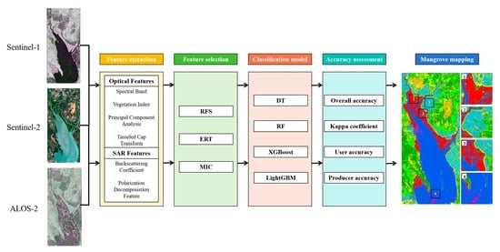
Graphical Abstract

1. Introduction

Mangroves are woody vegetation communities distributed along the tropical and subtropical intertidal zones, with high productivity and large carbon stocks [1]. They are found at the marine–terrestrial interface and are known as a specific ecosystem that provide great ecosystem services, such as climate regulation, biodiversity conservation, and water purification [2]. Despite their ecological importance and value, the total area of mangrove forests continues to decline due to human activities and climate change [3]. In the last two decades of the 20th century, about 35% of the world’s mangrove forests were lost [4]. A mangrove forest is also vulnerable to a variety of threats, including invasion by non-native species, human activities, and natural disasters, which have led to ecological imbalances and declined biodiversity. Therefore, accurate and timely spatial distribution information of mangrove forests is of great significance for mangrove conservation and restoration.
Due to the harsh mangrove growing environment and the poor accessibility caused by frequent tidal inundation, dense aboveground roots, and muddy soils, collecting observations through field surveys is challenging [5]. Remote sensing technology provides a new way and is considered effective in mangrove mapping. Selecting the appropriate remote sensing data source is crucial to the mapping of mangroves. Currently, the remote sensing data used for mangrove mapping mainly include optical and synthetic aperture radar (SAR) data [6]. Although multispectral data in optical imagery have the advantages of long time series and a large scale, their spectral resolution is usually lower, and they are susceptible to adverse meteorological conditions such as cloud cover. Hyperspectral data are suitable for the fine classification of mangrove forests, but currently, insufficient data are available for long-term and large-scale observation. SAR data are sensitive to the dielectric properties of objects and can provide unique information that optical imagery lacks. Additionally, SAR data are not affected by cloud cover; however, noise is often observed, and the number of available polarization modes is limited. Hence, some scholars have conducted research on mangrove mapping using multi-source remote sensing data. For example, Jhonnerie et al. [7] combined spectral reflectance, spectral transformation, and SAR features to map mangroves, achieving a highest overall accuracy of 81.1%. Ghorbanian et al. [8] demonstrated the effectiveness of multi-source remote sensing data (i.e., Sentinel-2 + Sentinel-1) in mangrove mapping. Abdel-Hamid et al. [9] assessed the contributions of various features derived from optical datasets, including vegetation indices, principal component analysis (PCA), and gray-level co-occurrence matrix (GLCM) textures and polarimetric SAR (PolSAR) parameters extracted from the ALOS/PALSAR data. The inclusion of texture features and PolSAR parameters improved the overall accuracy of the classification, achieving a highest overall accuracy (OA) of 84.30%. In summary, utilizing multi-source remote sensing data to extract the spectral, texture, and structural features of mangroves can improve the accuracy of mangrove recognition. However, despite the potential advantages of multi-source data, these studies often utilized traditional feature extraction and classification methods, lacking novel algorithms and techniques for multi-source data analysis. In addition, the lack of effective feature selection methods may lead to data redundancy and dimensionality issues, which can affect both the accuracy and interpretability of the extraction results. Therefore, the accurate mapping of mangrove forests over large-scale areas remains a challenging task in terms of combining multi-source remote sensing data.
Identifying and selecting classification features represent a decisive factors for the success of mangrove remote sensing classification. With the increased support of multi-source remote sensing big data, the feature variables currently used for mangrove forest recognition include electromagnetic spectral features, spatial features, temporal features, as well as other auxiliary geoscientific features such as digital elevation models (DEMs) [10]. On the one hand, a single type or source of data is insufficient to effectively express the complex features of mangrove forests and cannot fully meet the requirements. On the other hand, using an excessive number of feature variables can negatively impact the classification accuracy and efficiency [11]. Therefore, it can be seen that the extraction and optimization of multiple feature variables through the integration of multi-source remote sensing information will be one of the key and challenging areas for the intelligent extraction of mangrove information in the future. Suitable feature selection methods can be applied to address these problems. Regarding evaluation criteria, feature selection methods can be broadly divided into three categories: filter, embedded, and wrapper methods (Table 1). Filter methods score individual features based on relevance and set the number of features to be selected, and the wrapper methods are based on machine learning algorithms to evaluate the effectiveness of feature subsets [12]. These methods can detect the interrelationships between multiple features and select the optimal feature subset. Some researchers have explored the application of these algorithms in mangrove classification. Tang et al. [13] utilized the maximal information coefficient (MIC) to measure the nonlinear and non-functional relationships between features and eliminate redundant and irrelevant features, thereby improving diagnostic accuracy. Fei et al. [14] used random forest (RFS) to screen the extracted features and determine the optimal number of features and sensitive bands in classifying cotton. In general, current research on feature selection for mangrove classification mostly focuses on selecting the optimal feature set through methods such as multifactor variable participation and single-feature selection. The applicability of different classification features and combination modes, as well as feature selection methods, for the identification of mangroves has been rarely reported [15].
An appropriate algorithm is also a key step for mangrove mapping. In terms of classification methods, machine learning (ML) algorithms have been widely used in mangrove mapping due to their efficient computational ability and excellent classification results. Previous studies have utilized a range of classification techniques (Table 1), such as maximum likelihood classification (MLC) [16], decision tree (DT) [17], random forest (RF) [18], and support vector machine (SVM) [19]. Compared to other ML algorithms, ensemble learning (EL) algorithms led by DT and RF stand out in terms of their more significant generalization performance and more accurate results. Jhonnerie et al. [7] used RF and MLC algorithms to map mangroves and found that the RF algorithm produced better results and could also reduce noise in the classification results compared to MLC algorithms. Abdel-Hamid et al. [9] tested three non-parametric ML algorithms for mangrove mapping: RF, SVM, and DT. They found that RF had the highest performance in the integrated optical and SAR data classification, followed by DT and SVM in last place. Extreme gradient boosting (XGBoost) and light gradient-boosting machine (LightGBM) are new EL algorithms that have been developed in recent years. These algorithms have been successfully employed in some remote sensing ecological evaluations due to high accuracy, great computational power, and extremely fast computational speed [20]. Miao et al. [21] compared three machine learning models (XGBoost, RF, and LightGBM) in estimating three leaf nutrients (carbon, nitrogen, and phosphorus) in mangroves. The results showed that XGBoost had great potential for accurately estimating mangrove leaf nutrients using seasonal Sentinel-2 images. Su et al. [22] utilized the LightGBM algorithm to estimate time series chlorophyll-a (chl-a) concentration in Fujian’s coastal waters using multitemporal Ocean and Land Color Instrument (OLCI) data and in situ data. The results confirmed that the LightGBM model outperforms the traditional methods and OLCI chl-a products. However, XGBoost and LightGBM have rarely been applied in mangrove mapping [23], and their performance and applicability need to be further evaluated further to determine their superiority over traditional algorithms.
Based on the above analysis, this study took the Zhanjiang Mangrove National Nature Reserve, China, as the study area, aiming to extract mangrove information and map mangroves with high precision. The specific objectives were as follows: (1) comparing the effects of three feature selection methods (RFS, ERT, and MIC) and four machine learning algorithms (DT, RF, XGBoost, and LightGBM) on the classification accuracy of mangrove forests; (2) identifying the sensitive features of multi-source remote sensing data (Sentinel-2 optical multispectral data, and C-band Sentinel-1 and L-band ALOS-2 SAR data) for mangrove classification; (3) providing recommendations regarding the appropriateness of remote sensing data and the selection of the classification methods for mapping mangroves accurately and efficiently. Our study will contribute to the formulation of policies related to the protection and management of mangrove resources. The detailed workflow is shown in Figure 1.

2. Materials

2.1. Study Area

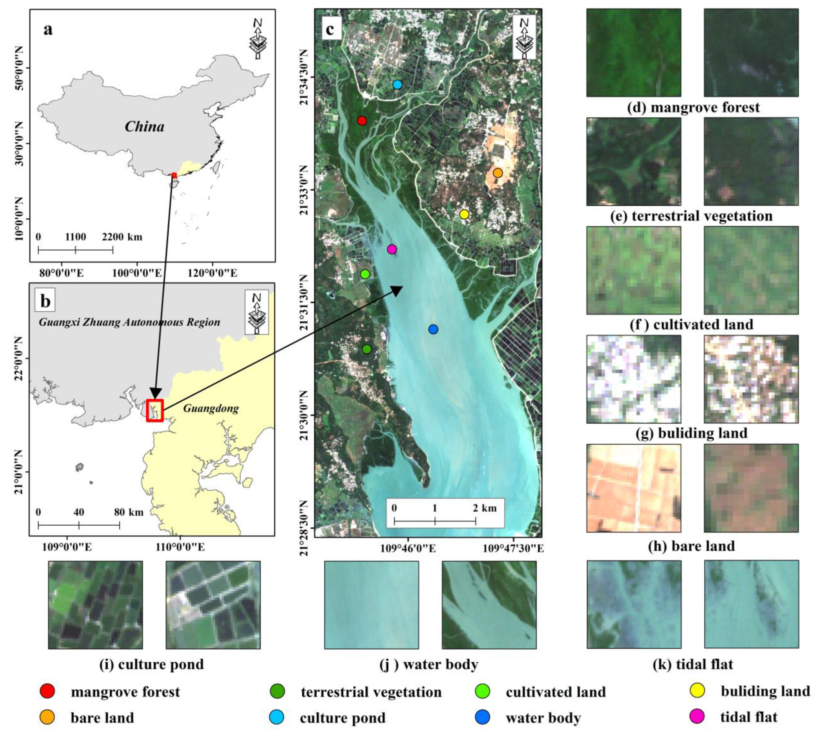
The Gaoqiao Mangrove Reserve (GMR) is the largest mangrove nature reserve in China and is located in Zhanjiang City, Guangdong Province. South subtropical monsoon marine climate is prevalent in this area. The annual average temperature is 23 °C, with an extreme maximum temperature of 38 °C in July and an extreme minimum temperature of 15 °C in January. The average annual precipitation is 1700~1800 mm, mainly concentrated from May to September. The area spans three types of tidal patterns: diurnal, semidiurnal, and mixed tides. This area has clay sediments and complex tidal channels that provide good environmental conditions for mangrove plants and other marine organisms. The mangroves of the reserve are mainly located in the eastern estuary of Yingluo Bay, from freshwater to open bay coastal areas. There are 8 true mangrove species, 13 semi-mangrove species, and 5 introduced mangrove species in the reserve. The GMR and its adjacent areas were selected for our study (Figure 2).

2.2. Data

2.2.1. Satellite Data and Preprocessing

Sentinel-2 (S2) is a high-resolution multispectral satellite mission, which consists of two satellites (2A and 2B) and was launched by Vega in June 2015 and March 2017, respectively. The Sentinel-2 satellite carries a multispectral imaging instrument, which has 13 spectral bands and provides images with resolutions of 10 m, 20 m, and 60 m. It has been widely used in ecological environment monitoring, vegetation health monitoring, and crop yield assessment [21].
Sentinel-1 (S1) is an earth observation satellite in the Copernicus Program of the European Space Agency. It consists of two satellites (1A and 1B) and carries a C-band dual-polarized synthetic aperture radar with VV (vertical transmit and vertical receive) and VH (vertical transmit and horizontal receive) polarization modes. Sentinel-1’s data products are acquired in multiple imaging models and are distributed at three levels of processing. It is mainly used in flood monitoring, ground surface settlement, and deformation monitoring [30].
ALOS-2 (A2) radar satellite was launched in May 2014 by the Japan Aerospace Exploration Agency (JAXA). It is equipped with a PALSAR-2 sensor, operates in the L-band, and has three observation modes (spotlight, stripmap, and scanSAR) with varying spatial resolutions and single, dual, and quad polarization. It can work all day under any weather conditions and is widely used in natural disaster monitoring, soil parameter inversion, and other fields [31].
The details of the data used in this study are shown in Table 2. The Sentinel-2B Level-1C data were acquired from the United States Geological Survey (USGS) (http://earthexplorer.usgs.gov, accessed on 22 August 2022) and were processed to Level-2A data using the Sen2Cor module. All the multispectral bands were resampled to 10 m spatial resolution using the Sen2Res module in SNAP9.0. The Sen2Res is a super-resolution image reconstruction method proposed for Sentinel-2 using shared geometric information between adjacent pixels, which not only maintains spectral consistency but also improves image sharpness and spatial detail. SNAP 9.0 software was used to process the Sentinel-1A data, including orbit correction, radiometric calibration, multi-looking, speckle filtering, and polarization decomposition, and finally, we used SRTM (Shuttle Radar Topography Mission) DEM data for terrain correction and resampled to 10 m spatial resolution. The preprocessing of ALOS-2 data is similar to that of Sentinel-1A data.

2.2.2. Sample Datasets

In this study, samples were selected via visual interpretation from high-resolution Google Earth images and were collected in a field survey, which included eight classes: mangrove forest, terrestrial vegetation, cultivated land, building land, bare land, culture pond, water body, and tidal flat. ArcGIS10.4 software was utilized to select 1000 sample points and determine the category attribute of each point based on high-resolution images and field survey data. To ensure sufficient data for both training and testing sets based on the random numbers and maintain consistency across all experimental schemes, a 7:3 ratio was selected to divide the training and testing sets, which is a commonly used ratio in the field of machine learning [32]. The distribution and number of sample points for each class are shown in Figure 2 and Table 3.

3. Methods

3.1. Feature Extraction

3.1.1. Multispectral Image Features

A total of 12 spectral bands and 15 indices (Table 4) of S2 were selected as spectral features in our study. Moreover, the first three bands of the principal component analysis (PCA) and brightness, greenness, and wetness components of the Tasseled Cap Transform (TCT) were also extracted from the Sentinel-2 data to improve the mangrove classification accuracy.

3.1.2. Polarimetric SAR Features

Polarimetric SAR data can provide the spatial structure features of mangroves. Related studies showed that the backscattering coefficient and polarization decomposition parameters of polarimetric SAR can be used to improve the accuracy of mangrove extraction [19]. In this study, SNAP 9.0 was used to extract the backscattering coefficients of two different polarization modes and three polarization decomposition features of two different bands of polarimetric SAR data (Table 5).

3.2. Feature Selection

In order to identify the features sensitive to mangrove extraction, in this study, the performance of three feature selection algorithms was compared: random forest (RFS), extremely randomized tree (ERT), and maximal information coefficient (MIC).

3.2.1. Random Forest (RFS)

RFS is an ML algorithm that integrates multiple decision trees, which can utilize the importance of features to evaluate features [47]. The basic idea is to calculate the contribution value of each feature to each tree in the RF, then take the average value to compare and sort the contribution value between the features, which can be measured with the Gini index and out-of-bag error rate. In this study, the Gini index was used to measure the importance of features; the details are as follows:
V I and G I indicate the feature importance and the Gini index; there are m features ( X 1 ,   X 2 ,   X 3 , ,   X m ). Then, they calculate the Gini index V I j G i n i for each feature X j , which is the average change in the j th feature’s splitting impurity across all nodes in the RF. The Gini index is defined as follows:
G I m = k = 1 K k k p m k p m k = 1 k = 1 K p m k 2
where K represents the number of categories; p m k indicates the proportion of the k th category in node m .
The importance of feature X j in node m   , that is, the change in the Gini index before and after node m branches, is defined as follows:
V I j G i n i = G I m G I l G I r
where G I l and G I r represent the Gini index of the two new nodes after branching.

3.2.2. Extremely Randomized Tree (ERT)

ERT is an EL-based algorithm; similar to RFS [48], it integrates multiple decision trees for scoring, votes according to the average of the predicted values of each decision tree, and calculates the branch contribution of features to each tree to evaluate feature importance. This method addresses the problem of decision tree similarity in RFS. Each tree of ERT is based on all training samples, which ensures the utilization of training samples. ERT introduces greater randomness in node partitioning by selecting a subset of features randomly at each node during segmentation to ensure the difference between each decision tree. Therefore, the variance of the decision tree is reduced, and the generalization ability is improved [49].

3.2.3. Maximal Information Coefficient (MIC)

Proposed by Reshef et al. [50], MIC is a method to measure the correlation between variables. For other correlation measures, it has better fairness and extensiveness, so it is neither affected by outliers nor limited to specific function types, and can explore potentially related variable pairs [51]. MIC is calculated using mutual information and mesh generation, where mutual information is the amount of information contained in one random variable about another random variable. In this study, the mutual information I Y ; X between ground object categories ( Y ) and classification features ( X ) is defined as follows:
I Y ; X = P Y , X l o g 2 P Y , X P Y P X
where P Y , X is the joint probability density Y and X ; P Y indicates the marginal probability density of Y ; and P X indicates the marginal probability density of X .
With Equation (3), the MIC is defined as follows:
M I C Y ; X = max ab < B n I Y ; X l o g 2 m i n a , b
where a is the number of grids divided in the Y direction; b is the number of grids divided in the X direction; n indicates the sample number; and B n ’s default setting is n 0.6 .

3.2.4. Determining the Optimal Number of Features

The optimal number of features is determined based on the feature importance (RFS and ERT) and maximal mutual information value (MIC). The details are as follows:
Step 1: Obtain the feature importance or maximal mutual information value based on the divided validation sets and training sets.
Step 2: Sort the importance or maximum mutual information values from high to low and select the first m features in turn.
Step 3: Based on the first m features and training sets, construct the classification model and use the validation sets to calculate its overall accuracy (OA). The OA will change with the increasing number of features. Take the number corresponding to its maximum value as the optimal number of features.

3.3. Image Classification with Machine Learning Algorithms

In this study, four ML algorithms were employed for image classification: decision tree (DT), random forest (RF), extreme gradient boosting (XGBoost), and light gradient-boosting machine (LightGBM).

3.3.1. Decision Tree (DT)

A DT is a non-parametric classification method that progressively subdivides the data into a decision tree structure in the form of a binary tree through recursive analysis [52]. Because it is simple and easy to explain, it has been widely used in remote sensing classification studies. The process of classification with a DT is to start from the root node and select the output branch according to the value of the corresponding feature attributes of the sample until it reaches the leaf node, and take the result of the leaf node as the final result. To characterize the merit of attribute selection at branching in the DT, the indicator information gain is often introduced, defined as the difference between the information entropy E n t D of set D and the information conditional entropy E n t D a of D under the condition of a given feature a; the formula is defined as follows:
G a i n D , a = E n t D E n t D a = E n t D v = 1 V D v D E n t D v
E n t D = k = 1 K P k l o g 2 P k
where P k is the proportion of samples of category k in sample set D ; D v indicates the number of samples contained in the v th branch node in the feature a .

3.3.2. Random Forest (RF)

RF is an EL algorithm proposed based on the bagging method; consisting of multiple decision trees, it treats each decision tree as an estimator and selects the optimal estimator with the highest votes as the final prediction result of the model [29]. Multiple decision trees are used to complete the task together, which can effectively solve the problems of the underfitting and overfitting of single-decision-tree classification results and achieve better accuracy [47]. Its final prediction result can be expressed as follows:
H x = a r g m a x y i = 1 K I h i X = Y
where H x is the final prediction result, I h i X = Y indicates the characteristic function, h i indicates the single DT, and Y represents the output variable.

3.3.3. Extreme Gradient Boosting (XGBoost)

XGBoost was proposed based on the gradient-boosting decision tree (GBDT) [53]. Compared to the traditional GBDT algorithm, XGBoost carries out improvements such as a second-order Taylor expansion of the loss function and adding a regularization item to make the algorithm faster and more accurate. XGBoost uses a DT as a weak classifier and splits by continuously adding DTs to form a new function to fit the residuals of previous predictions based on the newly generated DT [53]. The sample input to each DT will find the corresponding leaf nodes that can obtain a prediction result, and the scores of each DT will be summed up to obtain the final prediction result. Its objective function is as follows:
O b j = i = 1 N L y i , y ^ i + j = 1 T Ω f j
where i is the i th sample in the sample dataset, N presents the total number of samples, T represents all established trees, y i and y ^ i are the true and predicted values of the samples, L y i , y ^ i indicates the loss function, and Ω f j indicates the complexity of the j th tree, also known as the regularization item, which is used to control the complexity of the model to prevent overfitting. Its complexity is defined as follows:
Ω f = Υ T + 1 2 λ j = 1 T ω J 2
where Υ and λ are hyperparameters, T is the number of leaf nodes, and ω J 2 represents the square of the value of each leaf node.

3.3.4. Light Gradient-Boosting Machine (LightGBM)

LightGBM is a gradient-boosting framework proposed based on a decision tree, which supports efficient parallel training and has the advantages of faster training speed, less memory consumption, and higher accuracy [20]. The traditional GBDT algorithm needs to traverse all the data in each iteration, which is highly space- and time-consuming. In order to avoid these shortcomings and speed up the model training without affecting the accuracy, LightGBM performs the following optimizations: (1) the histogram algorithm, replacing the XGBoost pre-sorting algorithm, reduces the number of candidate classification points; gradient-based one-side sampling (GOSS), which reduces the complexity of calculating the gain of the objective function by sampling the samples; (2) exclusive feature bunding (EFB), which reduces the calculation complexity by reducing the number of features used to construct the histogram. The objective function of LightGBM is the same as XGBoost, which uses the greedy algorithm to select the one with the largest information gain after splitting, and the gain function is as follows:
G a i n = 1 2 G L 2 H L + λ + G R 2 H R + λ G L + G R 2 H L + H R + λ Υ
where G L and G R are the first derivative statistics of the loss function of the left and right leaf nodes; H L and H R indicate the second derivative statistics of the loss function of the left and right leaf nodes.

3.4. Accuracy Assessment

In this study, the confusion matrix is used to evaluate the accuracy of the classification results, and the specific evaluation indexes include the overall accuracy (OA), producer accuracy (PA), user accuracy (UA), and kappa coefficient. The specific formulas are as follows:
O A = i = 1 n x i i N
P A = x i i x + i
U A = x i i x i +
K a p p a = N i = 1 n x i i i = 1 n x i + x + i N 2 i = 1 n x i + x + i
where n is the number of categories, N is the total number of samples, x i i   indicates the number of samples in row i   and column i , x i +   indicates the sum of category i in the classification result, and x + i indicates the sum of true samples in category i .

4. Results

4.1. Classification with a Single Data Source

4.1.1. Feature Selection Results

In this study, a total of 43 features were extracted from S2, S1, and A2 data sources, three feature selection methods (RFS, ERT, and MIC) were employed to rank all features, and finally, the performance of the three methods was evaluated based on four ML models (DT, RF, XGBoost, and LightGBM).
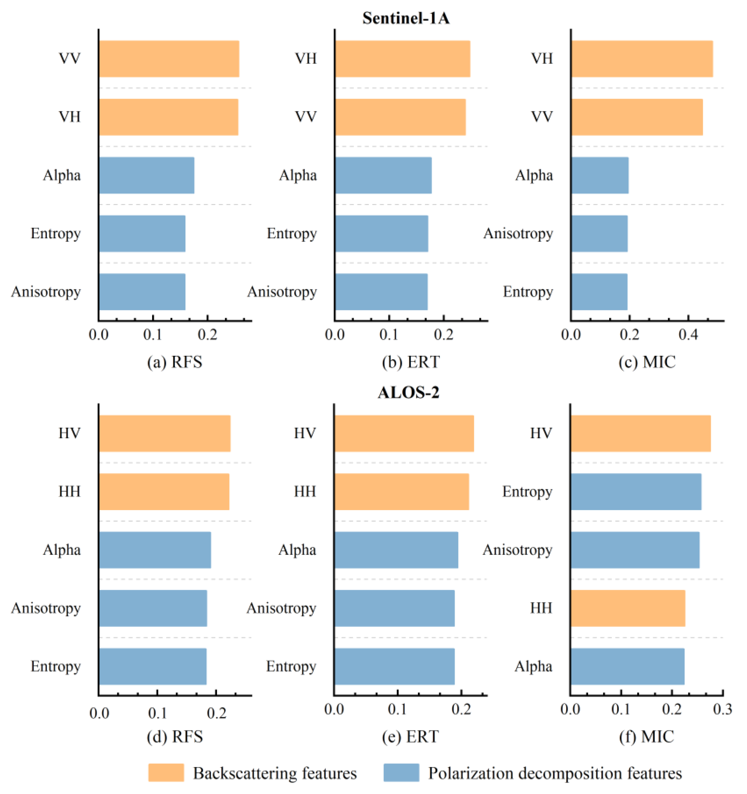
As shown in Figure 3, among the top ten features, more spectral features were selected than indices and other features: RFS filtered six spectral features and four vegetation and water indices; ERT filtered six spectral properties, three vegetation and water indices, and one TCT component; and MIC filtered nine vegetation and water indices and one TCT component. Table 6 shows that ERT and RFS produced better accuracy results than MIC, which indicates that spectral bands have a significant impact on classification, while vegetation and water indices have a minimal impact. Among the top ten features screened by RFS and ERT, all six spectral features were B1, B2, B3, B4, B11, and B12, among which B2 and B12 were more important than the other four bands, and MNDWI was the most important spectral index. In terms of polarimetric SAR features (Figure 4), the features screened via all three methods, the importance of backscattering features was higher than that of polarization decomposition features, but in the ALOS-2 data, the difference between these two types of features was not obvious.
Table 6 shows the accuracy when using the optimal number of features selected via three feature selection methods for the four ML models. The performance of RFS and ERT was better than that of MIC. RFS and ERT had similar classification performance because they are both ML algorithms based on the decision tree. In the DT and RF classification models, the ERT method achieved higher accuracy compared to RFS when the number of selected features was similar. In contrast, for the XGBoost and LightGBM classification models, the accuracy of the ERT method was slightly lower than that of the RFS, but the ERT algorithm reduced the number of selected features significantly, resulting in a more optimized classification model. Hence, ERT was considered the best feature selection method among the three feature selection methods evaluated in this study.

4.1.2. The Accuracy of Classification for a Single Data Source

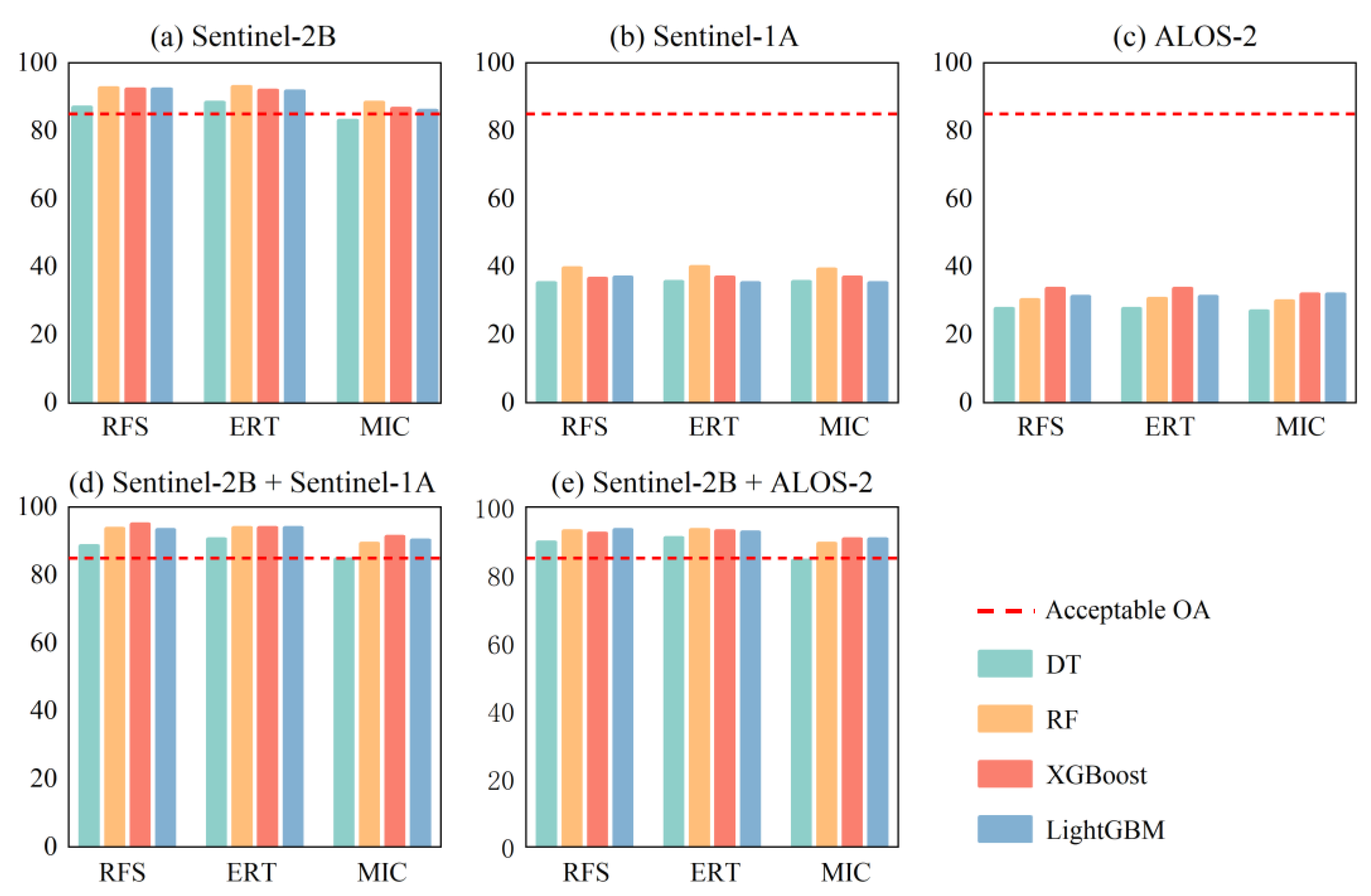
Table 6 and Figure 5a–c summarize the accuracy results for using a single data source. The results show that the S2 data all outperformed the acceptable OA, except in the MIC and DT methods, where the accuracy was below the acceptable OA, and for the SAR data, where the results were significantly lower than the acceptable OA, the S2 data had better performance than both SAR data. Specifically, the OA of the S2 data ranged from 83.00% to 93.00%, and the kappa ranged from 0.804 to 0.915. Based on the ERT and RF methods, using the S2 data achieved the highest accuracy (OA = 93.00%; kappa = 0.919). In the case of SAR data, the classification accuracy decreased substantially: the highest OA of the S1 data with the ERT and RF methods was only 40.00%, and the highest OA of the A2 data with the ERT and XGBoost methods was 33.67%.

4.2. Classification with Combined Data

Two combination schemes (SC: Sentinel-2B and Sentinel-1A; SL: Sentinel-2B and ALOS-2) were used to explore the potential of combining optical and dual polarimetric SAR for mangrove classification.
The accuracy results derived from the two schemes are summarized in Table 7 and Figure 5d,e. All results in both schemes exceeded the acceptable OA, except in the DT and MIC methods, and the results from the combined data were better than the single-data-source results. Combining the S2 and S1 data increased the OA by 1–4.67%, and the kappa increased by 0.012–0.054 compared to using S2 data in isolation. The best classification result was generated with RFS feature selection and the XGBoost model (OA = 95%; kappa = 0.942).
For the SL scheme, the OA and kappa increased by 0.33–4.67%, 0.004–0.054, respectively. The classification result achieved by the RFS feature selection and LightGBM model and ERT feature selection and RF model had the highest OA and kappa of 93.33% and 0.923, respectively. In both schemes SC and SL, the MIC feature selection method and DT model performed the worst among all classification results, with the lowest OA and kappa of 84.33% and 0.819, respectively. Although the XGBoost classification model combined with the RFS method produced the highest classification accuracy, the ERT method consistently performed well across all four classification models. Moreover, when considering the feature numbers and classification accuracy, the overall performance of the ERT method was better than that of the RFS method.
The combination with the highest accuracy of the two schemes was selected separately to calculate their feature importance scores (Figure 6). In the two schemes, the importance of the multispectral features was significantly higher than that of dual-polarized SAR features. Overall, this was not as much as the contribution of multispectral data, yet the addition of dual-polarized SAR data could improve the classification accuracy to some degree.

4.3. Comparison between C-Band and Dual-Polarized SAR and L-Band Dual-Polarized SAR

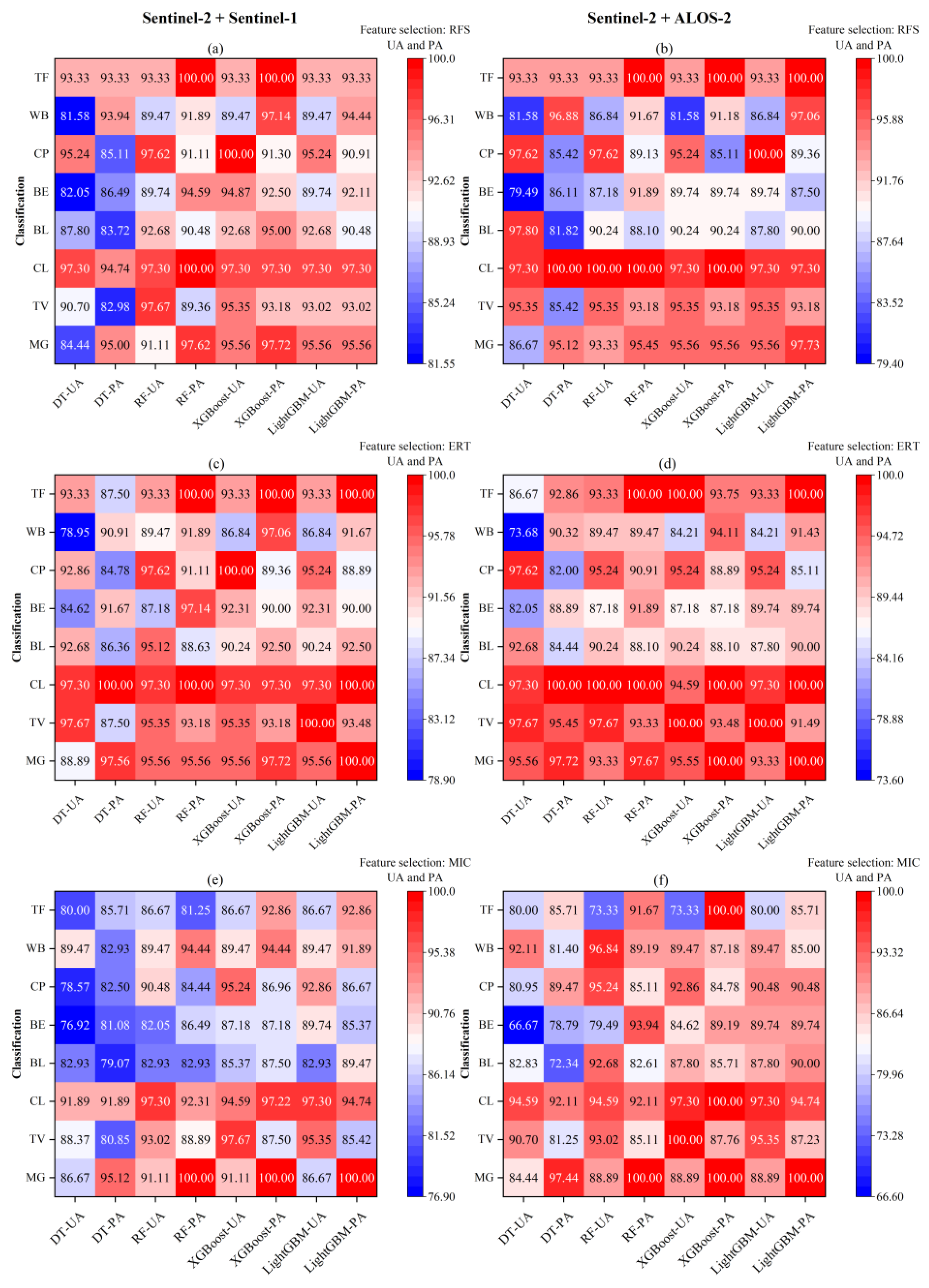
The PA and UA for each class in the two schemes (SC and SL) were calculated based on the combined features of the three feature selection methods and four ML algorithms, respectively, which are presented in the heat maps (Figure 7). For scheme SC, the PA and UA of each class by ERT were overall better than RFS and MIC. For scheme SL, RFS and ERT performed better than MIC, with little difference.
It can be seen from Figure 7 that almost all categories in the two schemes achieved a high PA and UA of more than 80%, which demonstrated the high applicability of both proposed schemes. In terms of mangrove forests, SL obtained the highest accuracy (PA = 97.72%, 97.67, 100.00%, and 100.00% for DT, RF, XGBoost, and LightGBM, respectively), followed by SC (PA = 97.56%, 95.56%, 97.72%, and 100.00% for DT, RF, XGBoost, and LightGBM, respectively). For terrestrial forest, the PA and UA of scheme SL were also higher than SC. The cultivated land had the highest PA and UA among the eight land cover categories for both schemes (97.00–100.00%), except for the UA of 94% for the XGBoost classification algorithms in SC. This may be because the scattering mechanism of cultivated land was mainly surface scattering, with a significantly lower backscattering coefficient than mangrove forest and terrestrial forest. Based on four ML algorithms, both schemes were moderately successful in distinguishing between building land and bare land. The PA and UA of building land and bare land in SC were higher than those of SL. Meanwhile, both schemes also produced a higher PA and UA (>80%) in distinguishing between culture ponds and water bodies in the three ML algorithms of RF, XGBoost, and LightGBM. However, SC produced a higher PA and UA compared to SL, except for the DT classification algorithm, which produced a slightly lower UA (92.86% for SC; 97.62% for SL) when differentiating culture ponds. For tidal flats, which had an insufficient number of sample points selected due to their small area in this region, the PA and UA of both schemes were not significantly different, but a higher classification accuracy could be maintained.
In general, both schemes performed well in the classification. The result proved that the SL scheme outperformed SC in distinguishing vegetation (mangrove forest, terrestrial forest, and cultivated land), and SC was slightly better at distinguishing building land, bare land, culture ponds, and water bodies.

4.4. Mapping the Classification Results of Two Schemes Based on Four Machine Learning Algorithms

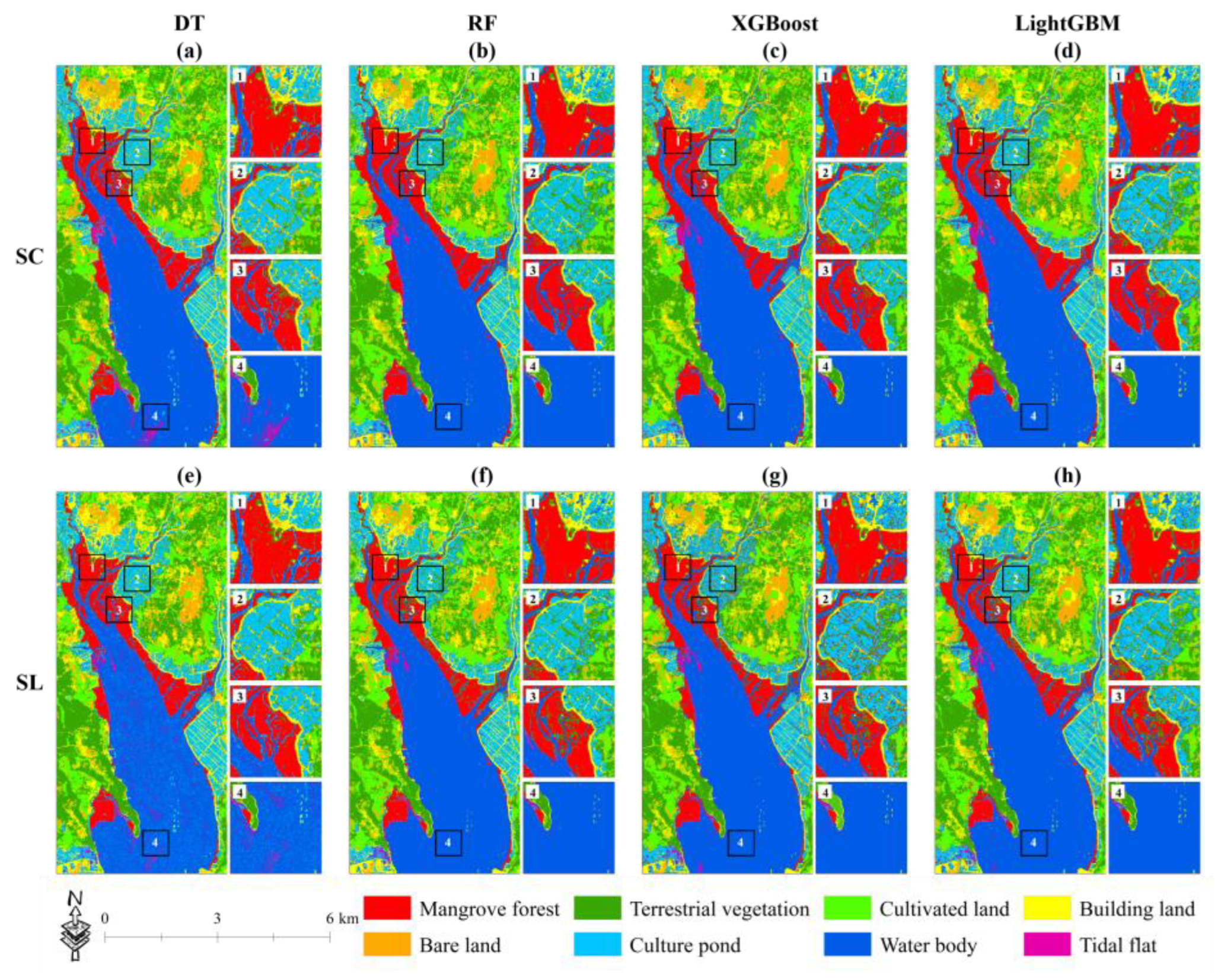
Based on the features selected via the ERT feature selection method, the classification results of the two schemes were mapped using four ML algorithms, respectively (Figure 8). The visual assessment showed high consistency with our field survey. In this study area, mangrove forests were mainly distributed near the central coast, and a small portion were distributed in the southern part of the study area, whose outer sides were surrounded by water bodies and most of the inner sides were enclosed by culture ponds. The classification results with combined data of both SC and SL were satisfactory. However, the results were not perfect. In the SC scheme, for the result of the DT model (Figure 8a), there were some obvious misclassifications: mangrove forests were misclassified as terrestrial vegetation in the central region, water bodies were misclassified as tidal flats and culture ponds in the southern region, and the other three models were better than the DT model for the classification of water bodies. In the results of LightGBM (Figure 8e), there was some terrestrial vegetation near culture ponds that was misclassified as mangrove forests. The results of RF and XGBoost were similar, while in the SL scheme, some mangrove forests were misclassified as terrestrial vegetation in the central region compared to the SC scheme. In the results of DT (Figure 8e), a large number of water bodies were misclassified as culture ponds and tidal flats. In the classification of culture ponds in the central region, the results were better than the other three classification models. In the results of XGBoost (Figure 8g), more land forests near culture ponds were misclassified as mangroves, and mangroves close to rivers were misclassified as land forests compared to the other three ML algorithms. In the extraction of mangrove interiors, RF and LightGBM were slightly better than DT and XGBoost. Combining the overall accuracy (Table 7) and classification results (Figure 8), the overall classification result of SC was better than SL. Among the four ML algorithms, DT performed the worst in two schemes, and LightGBM, RF, and XGBoost performed better in the two schemes.

5. Discussion

5.1. The Contribution and Sensitive Features of Optical and SAR Images

A comparative analysis of mangrove classification results using single optical or SAR remote sensing data shows that the S2 optical satellite data performed significantly better than S1 and A2 SAR data (Table 6). Hence, it is recommended that optical satellites with high spatial and temporal resolution should be preferred for mangrove monitoring and mapping whenever available. However, in cases where insufficient optical data are available, SAR data can serve as an effective supplementary data source for mangrove mapping. Our results show that combining optical and SAR data can improve the accuracy of mangrove mapping to a certain extent (0.33% to 4.67%). Although the degree of improvement in accuracy may not be significant, it is essential for the research of mangrove mapping in a larger area. This is consistent with some previous research findings. Aja et al. [54] evaluated mangrove classification performance in three scenarios: the classification of optical data only, radar data only, and a combination of optical and radar data. The results revealed that the scenario that combined optical and radar data performed better. Jhonnerie et al. [7] showed that the best result for mangrove mapping was obtained by the combination of Landsat 5 TM and ALOS PALSAR, with a 4.30% improvement in accuracy compared to optical data. It is worth noting that the effects of different wavelengths of SAR data on the identification of mangrove forests vary. Generally, longer wavelengths have a stronger capability to penetrate the vegetation canopy. C-band microwave signals interact more strongly with the upper leaves of the vegetation canopy. Their echoes are mainly from volume scattering in the vegetation canopy, which reflect more information about the canopy of grasses and crops [55]. L-band microwave signals penetrate through the upper layers of the canopy down to the tree trunks, and the scattering is largely from the multiple scattering caused by the ground and trunks; L-band signals are more sensitive to plant density, soil moisture, and inundation as compared to C-band signals [56]. Hess et al. [57] found that L-band SAR is mainly suitable for mapping forests, dense vegetation environments and woodland-dominated wetlands. This is consistent with the results of our study, where the combination of L-band data performed better in discriminating mangrove forests and terrestrial vegetation than C-band data (as shown in Figure 7), and was more effective in mapping and distinguishing forest vegetation.
Recognizing sensitive features extracted from mangrove information can effectively solve data redundancy and improve classification accuracy. In this study, 43 features were extracted from three types of remotely sensed data. Comparing the results of three feature selection methods (as shown in Table 6), it can be observed that the selection of preferred variables and their number are related to the classification algorithm chosen. The number of features preferred by the three feature selection methods in combination with the DT and RF classification strategies was almost equivalent. However, when combined with XGBoost and LightGBM, the ERT method reduced the number of features significantly, without having a considerable impact on accuracy. Additionally, ERT does not use random sampling, meaning that each decision tree uses the original training set, thus ensuring the stability of the data during training. Furthermore, ERT is able to select features with less variance compared to RFS, ensuring the validity and stability of the selected features [58]. Wang et al. [58] demonstrated the effectiveness of their feature selection method by screening the optimal feature subset based on the ERT algorithm with a higher classification accuracy than when all features were used. Both the XGBoost and LightGBM classification algorithms outperformed DT and RF in solving problems related to feature selection, overfitting, and local optimality. Therefore, combining XGBoost and LightGBM with ERT exhibits great potential for practical applications. The results of the feature selection process showed that ERT and RFS selected similar features with significantly better accuracy than the MIC method. In these two algorithms, the importance score ranking results (Figure 3) demonstrated that the visible band (B2, B3, B4) and shortwave infrared band (B11, B12) outperformed the other S2 bands in mangrove mapping, and the most sensitive vegetation indices were mainly constructed using these bands. The spectral response of the visible band is primarily associated with various pigments in vegetation, especially chlorophyll. Chlorophyll absorption peaks are observed in the blue (B2) and red (B4) bands, and a reflection peak appears in the green (B3) band, explaining why a significant amount of vegetation appears green. The sensitivity of the shortwave infrared band to the vegetation water content makes it particularly important in mangrove mapping. Compared to other vegetation cover, mangrove forests have a similar greenness, and the main difference lies in their leaf and canopy water contents. The amount of infrared wavelengths absorbed by vegetation primarily depends on the water content of the leaves. Due to the influence of environmental factors on mangrove survival, the water content of mangrove leaves and canopies is typically higher than that of most terrestrial vegetation cover. Therefore, mangrove forests and terrestrial vegetation can be distinguished well by using shortwave infrared bands, as is consistent with the findings of Yang et al. [59].

5.2. The Impact of Different Classification Algorithms on the Classification Accuracy

Based on the accuracy reported in Table 7, both the XGBoost and LightGBM algorithms achieved over 90.00% overall accuracy in all scenarios, demonstrating their superior performance in identifying mangrove forests. Additionally, it was found that the XGBoost and LightGBM algorithms outperformed the RF and DT algorithms in mapping mangrove forests. This is consistent with the findings of Jafarzadeh et al. [18] who used six EL methods, namely, adaptive boosting (AdaBoost), gradient-boosting machine (GBM), XGBoost, LightGBM, and RF, for the classification of remote sensing data. Their results indicated that in most cases, XGBoost and LightGBM provided more accurate results due to their improved version of EL algorithms. Remote sensing data possess complex spatial and spectral feature relationships. Both the XGBoost and LightGBM algorithms belong to the boosting EL category, which is adept at capturing complex nonlinear relationships and performs well in classification tasks. Furthermore, these boosting algorithms have been improved based on the gradient-boosting decision tree (GBDT), incorporating a second-order Taylor expansion of the loss function with an added regularization item, to achieve better accuracy while preventing overfitting. From Table 7, it can be observed that XGBoost and LightGBM had both high and low performance, which could be attributed to different selection features. However, in general, XGBoost outperformed LightGBM, which is in contrast to the findings of Fu et al. [60], who reported that LightGBM outperformed XGBoost in vegetation classification. This difference may be due to the different scales and sampling densities of the study area. However, most studies have shown that the XGBoost algorithm is more stable and performs better than LightGBM [21]. The basic principle of LightGBM is similar to XGBoost but has several improvements. The LightGBM algorithm utilizes a histogram-based approach to optimize the selection of split points, leading to reduced computational complexity and increased training speed, especially for large-scale datasets. Other optimization techniques, such as feature binding and parallel processing, are also biased towards large-scale datasets, which may not be as effective for sparse data. On the other hand, XGBoost uses a sparse-aware split lookup method that is more practical for processing sparse data, which is commonly encountered in the sampling of mangrove forest, as seen in this study.

5.3. Potential Application and Future Work

Based on the use of multi-source remote sensing data, the high-precision extraction of mangrove forests was achieved. However, our study also had some limitations and weaknesses. First, in our feature importance analysis of combining optical and SAR data (Figure 6), the features provided by both C-band and L-band SAR were found to be less useful in classification and did not fully utilize the advantages of multi-source data combination. Secondly, in our classification maps (Figure 8), due to image resolution issues, some of the terrestrial vegetation and culture pond categories were misclassified as mangrove forests in the central part of the study area where culture ponds intersected with terrestrial vegetation. The same problem occurred on some mangrove forests that were adjacent to bare land. For future work, other satellite images with similar or higher resolutions, such as qual-pol SAR images, OHS-1, and WorldView-2 images, could be explored for potential data for multi-source data combining. In addition, more variables closely related to plant functional trait characteristics, such as the water content of vegetation and the concentrations of C, N, and P, can be considered to further improve the accuracy and interpretability of the classification results.

6. Conclusions

This study demonstrated that the accurate mapping of mangrove forests in Gaoqiao Mangrove Reserve (GMR) can be achieved through the use of multi-source remote sensing data with feature selection methods and machine learning algorithms. Specifically, twenty-four classification schemes for mangrove forest mapping in GMR were established by combining Sentinel-2 optical data and SAR data from Sentinel-1 (C-band) and ALOS-2 (L-band) at different wavelengths, and three feature selection methods (RFS, ERT, and MIC) and four machine learning algorithms (DT, RF, XGBoost, and LightGBM) were applied. The main conclusions are as follows: (1) The ERT feature selection method was found to be the most suitable for selecting sensitive features in mangrove mapping. Among the features selected, the visible bands (blue, green, and red), shortwave infrared bands (SWIR1 and SWIR2), and vegetation indices (VARI and MNDWI) constructed from S2 images were found to contribute the most to the classification accuracy. (2) The XGBoost and LightGBM algorithms produced higher classification accuracy as compared to traditional algorithms (DT and RF), with an overall accuracy of above 90.00%. The XGBoost algorithm was found to perform optimally with the highest overall accuracy of 95.00% among all the classification algorithms. (3) The combination of multi-source data yielded better classification accuracy gains compared to using only a single data source alone. The overall effect of combining optical and C-band data was better than combining optical and L-band data. However, combining L-band data yielded better performance than C-band data in distinguishing between mangrove forests and terrestrial vegetation.

Author Contributions

Conceptualization and methodology, J.Z. and Z.S.; validation, J.Z., Z.S. and J.W.; formal analysis, J.Z., Z.S. and J.W.; investigation, J.W.; resources, J.Z., Z.S., J.W., J.M., D.Z. and A.T.; writing—original draft preparation, Z.S.; writing—review and editing, J.Z.; supervision, J.W.; project administration, J.Z.; funding acquisition, J.Z. and J.W. All authors have read and agreed to the published version of the manuscript.

Funding

This research was funded by the National Natural Science Youth Foundation of China, grant number 42301429, and the Shenzhen Science and Technology Program, grant number JCYJ 20210324093210029.

Data Availability Statement

Data are contained within the article.

Conflicts of Interest

The authors declare no conflict of interest. The funders had no role in the design of the study; in the collection, analyses, or interpretation of data; in the writing of the manuscript; or in the decision to publish the results.

References

  1. Thomas, N.; Lucas, R.; Bunting, P.; Hardy, A.; Rosenqvist, A.; Simard, M. Distribution and drivers of global mangrove forest change, 1996–2010. PLoS ONE 2017, 12, e0179302. [Google Scholar] [CrossRef] [PubMed]
  2. Abad-Segura, E.; Gonzalez-Zamar, M.D.; Vazquez-Cano, E.; Lopez-Meneses, E. Remote Sensing Applied in Forest Management to Optimize Ecosystem Services: Advances in Research. Forests 2020, 11, 969. [Google Scholar] [CrossRef]
  3. Son, N.T.; Chen, C.F.; Chang, N.B.; Chen, C.R.; Chang, L.Y.; Thanh, B.X. Mangrove Mapping and Change Detection in Ca Mau Peninsula, Vietnam, Using Landsat Data and Object-Based Image Analysis. IEEE J. Sel. Top. Appl. Earth Obs. Remote Sens. 2015, 8, 503–510. [Google Scholar] [CrossRef]
  4. Wang, L.; Jia, M.M.; Yin, D.M.; Tian, J.Y. A review of remote sensing for mangrove forests: 1956–2018. Remote Sens. Environ. 2019, 231, 111223. [Google Scholar] [CrossRef]
  5. Zhao, C.P.; Qin, C.Z. 10-m-resolution mangrove maps of China derived from multi-source and multi-temporal satellite observations. ISPRS J. Photogramm. Remote Sens. 2020, 169, 389–405. [Google Scholar] [CrossRef]
  6. Jia, M.M.; Wang, Z.M.; Zhang, Y.Z.; Mao, D.H.; Wang, C. Monitoring loss and recovery of mangrove forests during 42 years: The achievements of mangrove conservation in China. Int. J. Appl. Earth Obs. 2018, 73, 535–545. [Google Scholar] [CrossRef]
  7. Jhonnerie, R.; Siregar, V.P.; Nababan, B.; Prasetyo, L.B.; Wouthuyzen, S. Random Forest Classification for Mangrove Land Cover Mapping Using Landsat 5 TM and Alos Palsar Imageries. Procedia Environ. Sci. 2015, 24, 215–221. [Google Scholar] [CrossRef]
  8. Ghorbanian, A.; Zaghian, S.; Asiyabi, R.M.; Amani, M.; Mohammadzadeh, A.; Jamali, S. Mangrove Ecosystem Mapping Using Sentinel-1 and Sentinel-2 Satellite Images and Random Forest Algorithm in Google Earth Engine. Remote Sens. 2021, 13, 2565. [Google Scholar] [CrossRef]
  9. Abdel-Hamid, A.; Dubovyk, O.; Abou El-Magd, I.; Menz, G. Mapping Mangroves Extents on the Red Sea Coastline in Egypt using Polarimetric SAR and High Resolution Optical Remote Sensing Data. Sustainability 2018, 10, 646. [Google Scholar] [CrossRef]
  10. Zhao, C.P.; Jia, M.M.; Wang, Z.M.; Mao, D.H.; Wang, Y.Q. Identifying mangroves through knowledge extracted from trained random forest models: An interpretable mangrove mapping approach (IMMA). ISPRS J. Photogramm. Remote Sens. 2023, 201, 209–225. [Google Scholar] [CrossRef]
  11. Cheng, Q.; Varshney, P.K.; Arora, M.K. Logistic regression for feature selection and soft classification of remote sensing data. IEEE Geosci. Remote Sens. Lett. 2006, 3, 491–494. [Google Scholar] [CrossRef]
  12. Kohavi, R.; John, G.H. Wrappers for feature subset selection. Artif. Intell. 1997, 97, 273–324. [Google Scholar] [CrossRef]
  13. Tang, X.H.; Wang, J.C.; Lu, J.G.; Liu, G.K.; Chen, J.D. Improving Bearing Fault Diagnosis Using Maximum Information Coefficient Based Feature Selection. Appl. Sci. 2018, 8, 2143. [Google Scholar] [CrossRef]
  14. Fei, H.; Fan, Z.H.; Wang, C.K.; Zhang, N.N.; Wang, T.; Chen, R.G.; Bai, T.C. Cotton Classification Method at the County Scale Based on Multi-Features and Random Forest Feature Selection Algorithm and Classifier. Remote Sens. 2022, 14, 829. [Google Scholar] [CrossRef]
  15. Fu, B.; Liang, Y.; Lao, Z.; Sun, X.; Li, S.; He, H.; Sun, W.; Fan, D. Quantifying scattering characteristics of mangrove species from Optuna-based optimal machine learning classification using multi-scale feature selection and SAR image time series. Int. J. Appl. Earth Obs. 2023, 122, 103446. [Google Scholar] [CrossRef]
  16. Held, A.; Ticehurst, C.; Lymburner, L.; Williams, N. High resolution mapping of tropical mangrove ecosystems using hyperspectral and radar remote sensing. Int. J. Remote Sens. 2003, 24, 2739–2759. [Google Scholar] [CrossRef]
  17. Li, W.Z.; El-Askary, H.; Qurban, M.A.; Li, J.J.; ManiKandan, K.P.; Piechota, T. Using multi-indices approach to quantify mangrove changes over the Western Arabian Gulf along Saudi Arabia coast. Ecol. Indic. 2019, 102, 734–745. [Google Scholar] [CrossRef]
  18. Jafarzadeh, H.; Mahdianpari, M.; Gill, E.; Mohammadimanesh, F.; Homayouni, S. Bagging and Boosting Ensemble Classifiers for Classification of Multispectral, Hyperspectral and PolSAR Data: A Comparative Evaluation. Remote Sens. 2021, 13, 4405. [Google Scholar] [CrossRef]
  19. Zhen, J.N.; Liao, J.J.; Shen, G.Z. Mapping Mangrove Forests of Dongzhaigang Nature Reserve in China Using Landsat 8 and Radarsat-2 Polarimetric SAR Data. Sensors 2018, 18, 4012. [Google Scholar] [CrossRef]
  20. Ke, G.; Meng, Q.; Finley, T.; Wang, T.; Chen, W.; Ma, W.; Ye, Q.; Liu, T.-Y. LightGBM: A Highly Efficient Gradient Boosting Decision Tree. Adv. Neurol. 2017, 30, 52. [Google Scholar]
  21. Miao, J.; Zhen, J.N.; Wang, J.J.; Zhao, D.M.; Jiang, X.P.; Shen, Z.; Gao, C.J.; Wu, G.F. Mapping Seasonal Leaf Nutrients of Mangrove with Sentinel-2 Images and XGBoost Method. Remote Sens. 2022, 14, 3679. [Google Scholar] [CrossRef]
  22. Su, H.; Lu, X.M.; Chen, Z.Q.; Zhang, H.S.; Lu, W.F.; Wu, W.T. Estimating Coastal Chlorophyll-A Concentration from Time-Series OLCI Data Based on Machine Learning. Remote Sens. 2021, 13, 576. [Google Scholar] [CrossRef]
  23. Fu, B.; He, X.; Yao, H.; Liang, Y.; Deng, T.; He, H.; Fan, D.; Lan, G.; He, W. Comparison of RFE-DL and stacking ensemble learning algorithms for classifying mangrove species on UAV multispectral images. Int. J. Appl. Earth Obs. 2022, 112, 102890. [Google Scholar] [CrossRef]
  24. Guyon, I.; Elisseeff, A. An introduction to variable and feature selection. J. Mach. Learn. Res. 2003, 3, 1157–1182. [Google Scholar]
  25. You, M.; Liu, J.; Li, G.-Z.; Chen, Y. Embedded Feature Selection for Multi-label Classification of Music Emotions. Int. J. Comput. Intell. Syst. 2012, 5, 668–678. [Google Scholar] [CrossRef]
  26. Al-Ahmadi, F.S.; Al-Hames, A.S. Comparison of four classification methods to extract land use and land cover from raw satellite images for some remote arid areas, Kingdom of Saudi Arabia. Earth Sci. 2009, 20, 24. [Google Scholar] [CrossRef]
  27. Foody, G.M.; Mathur, A. A relative evaluation of multiclass image classification by support vector machines. IEEE Trans. Geosci. Remote Sens. 2004, 42, 1335–1343. [Google Scholar] [CrossRef]
  28. Maxwell, A.E.; Warner, T.A.; Fang, F. Implementation of machine-learning classification in remote sensing: An applied review. Int. J. Remote Sens. 2018, 39, 2784–2817. [Google Scholar] [CrossRef]
  29. Breiman, L. Random forests. Mach. Learn. 2001, 45, 5–32. [Google Scholar] [CrossRef]
  30. Shami, S.; Azar, M.K.; Nilfouroushan, F.; Salimi, M.; Reshadi, M.A.M. Assessments of ground subsidence along the railway in the Kashan plain, Iran, using Sentinel-1 data and NSBAS algorithm. Int. J. Appl. Earth Obs. 2022, 112, 102898. [Google Scholar] [CrossRef]
  31. Yamaguchi, Y.; Umemura, M.; Kanai, D.; Miyazaki, K.; Yamada, H. ALOS-2 polarimetric SAR observation of Hokkaido- Iburi-Tobu earthquake 2018. Ieice Commun. Express 2019, 8, 26–31. [Google Scholar] [CrossRef]
  32. Vrigazova, B. The Proportion for Splitting Data into Training and Test Set for the Bootstrap in Classification Problems. Bus. Syst. Res. J. 2021, 12, 228–242. [Google Scholar] [CrossRef]
  33. Datt, B. Remote sensing of chlorophyll a, chlorophyll b, chlorophyll a+b, and total carotenoid content in eucalyptus leaves. Remote Sens. Environ. 1998, 66, 111–121. [Google Scholar] [CrossRef]
  34. Huete, A.R.; Liu, H.Q.; Batchily, K.; van Leeuwen, W. A comparison of vegetation indices global set of TM images for EOS-MODIS. Remote Sens. Environ. 1997, 59, 440–451. [Google Scholar] [CrossRef]
  35. Sakamoto, T.; Van Nguyen, N.; Kotera, A.; Ohno, H.; Ishitsuka, N.; Yokozawa, M. Detecting temporal changes in the extent of annual flooding within the Cambodia and the Vietnamese Mekong Delta from MODIS time-series imagery. Remote Sens. Environ. 2007, 109, 295–313. [Google Scholar] [CrossRef]
  36. Rondeaux, G.; Steven, M.; Baret, F. Optimization of soil-adjusted vegetation indices. Remote Sens. Environ. 1996, 55, 95–107. [Google Scholar] [CrossRef]
  37. Tucker, C.J. Red and photographic infrared linear combinations for monitoring vegetation. Remote Sens. Environ. 1979, 8, 127–150. [Google Scholar] [CrossRef]
  38. Sripada, R.P.; Heiniger, R.W.; White, J.G.; Meijer, A.D. Aerial color infrared photography for determining early in-season nitrogen requirements in corn. Agron. J. 2006, 98, 968–977. [Google Scholar] [CrossRef]
  39. Huete, A.R. A soil-adjusted vegetation index (SAVI). Remote Sens. Environ. 1988, 25, 295–309. [Google Scholar] [CrossRef]
  40. McFeeters, S.K. The use of the normalized difference water index (NDWI) in the delineation of open water features. Int. J. Remote Sens. 1996, 17, 1425–1432. [Google Scholar] [CrossRef]
  41. Xu, H.Q. Modification of normalised difference water index (NDWI) to enhance open water features in remotely sensed imagery. Int. J. Remote Sens. 2006, 27, 3025–3033. [Google Scholar] [CrossRef]
  42. Gitelson, A.A.; Kaufman, Y.J.; Stark, R.; Rundquist, D. Novel algorithms for remote estimation of vegetation fraction. Remote Sens. Environ. 2002, 80, 76–87. [Google Scholar] [CrossRef]
  43. Crippen, R.E. Calculating the vegetation index faster. Remote Sens. Environ. 1990, 34, 71–73. [Google Scholar] [CrossRef]
  44. Roujean, J.-L.; Breon, F.-M. Estimating PAR absorbed by vegetation from bidirectional reflectance measurements. Remote Sens. Environ. 1995, 51, 375–384. [Google Scholar] [CrossRef]
  45. Gao, C.; Jiang, X.; Zhen, J.; Wang, J.; Wu, G. Mangrove species classification with combination of WorldView-2 and Zhuhai-1 satellite images. Natl. Remote Sens. Bull. 2022, 26, 1155–1168. [Google Scholar] [CrossRef]
  46. Cloude, S.R.; Pottier, E. A review of target decomposition theorems in radar polarimetry. IEEE Trans. Geosci. Remote Sens. 1996, 34, 498–518. [Google Scholar] [CrossRef]
  47. Saraswat, M.; Arya, K.V. Feature selection and classification of leukocytes using random forest. Med. Biol. Eng. Comput. 2014, 52, 1041–1052. [Google Scholar] [CrossRef]
  48. Geurts, P.; Ernst, D.; Wehenkel, L. Extremely randomized trees. Mach. Learn. 2006, 63, 3–42. [Google Scholar] [CrossRef]
  49. Wu, M.H.; Lin, N.; Li, G.J.; Liu, H.L.; Li, D.L. Hyperspectral estimation of petroleum hydrocarbon content in soil using ensemble learning method and LASSO feature extraction. Environ. Pollut. Bioavailab. 2022, 34, 308–320. [Google Scholar] [CrossRef]
  50. Reshef, D.N.; Reshef, Y.A.; Finucane, H.K.; Grossman, S.R.; McVean, G.; Turnbaugh, P.J.; Lander, E.S.; Mitzenmacher, M.; Sabeti, P.C. Detecting Novel Associations in Large Data Sets. Science 2011, 334, 1518–1524. [Google Scholar] [CrossRef] [PubMed]
  51. Sun, G.L.; Li, J.B.; Dai, J.; Song, Z.C.; Lang, F. Feature selection for IoT based on maximal information coefficient. Future Gener. Comput. Syst. 2018, 89, 606–616. [Google Scholar] [CrossRef]
  52. Friedl, M.A.; Brodley, C.E. Decision tree classification of land cover from remotely sensed data. Remote Sens. Environ. 1997, 61, 399–409. [Google Scholar] [CrossRef]
  53. Chen, T.; Guestrin, C. XGBoost: A Scalable Tree Boosting System. In Proceedings of the 22nd Acm Sigkdd International Conference on Knowledge Discovery and Datamining, San Francisco, CA, USA, 13–17 August 2016; pp. 785–794. [Google Scholar]
  54. Aja, D.; Miyittah, M.K.; Angnuureng, D.B. Quantifying Mangrove Extent Using a Combination of Optical and Radar Images in a Wetland Complex, Western Region, Ghana. Sustainability 2022, 14, 16687. [Google Scholar] [CrossRef]
  55. Tsyganskaya, V.; Martinis, S.; Marzahn, P.; Ludwig, R. SAR-based detection of flooded vegetation - a review of characteristics and approaches. Int. J. Remote Sens. 2018, 39, 2255–2293. [Google Scholar] [CrossRef]
  56. Mandianpari, M.; Salehi, B.; Mohammadimanesh, F.; Motagh, M. Random forest wetland classification using ALOS-2 L-band, RADARSAT-2 C-band, and TerraSAR-X imagery. ISPRS J. Photogramm. Remote Sens. 2017, 130, 13–31. [Google Scholar] [CrossRef]
  57. Hess, L.L.; Melack, J.M.; Simonett, D.S. Radar detection of flooding beneath the forest canopy: A review. Int. J. Remote Sens. 1990, 11, 1313–1325. [Google Scholar] [CrossRef]
  58. Wang, X.Z.; Tan, L.L.; Fan, J.C. Performance Evaluation of Mangrove Species Classification Based on Multi-Source Remote Sensing Data Using Extremely Randomized Trees in Fucheng Town, Leizhou City, Guangdong Province. Remote Sens. 2023, 15, 1386. [Google Scholar] [CrossRef]
  59. Yang, G.; Huang, K.; Sun, W.W.; Meng, X.C.; Mao, D.H.; Ge, Y. Enhanced mangrove vegetation index based on hyperspectral images for mapping mangrove. ISPRS J. Photogramm. Remote Sens. 2022, 189, 236–254. [Google Scholar] [CrossRef]
  60. Fu, B.L.; Zuo, P.P.; Liu, M.; Lan, G.W.; He, H.C.; Lao, Z.A.; Zhang, Y.; Fan, D.L.; Gao, E.R. Classifying vegetation communities karst wetland synergistic use of image fusion and object-based machine learning algorithm with Jilin-1 and UAV multispectral images. Ecol. Indic. 2022, 140, 108989. [Google Scholar] [CrossRef]
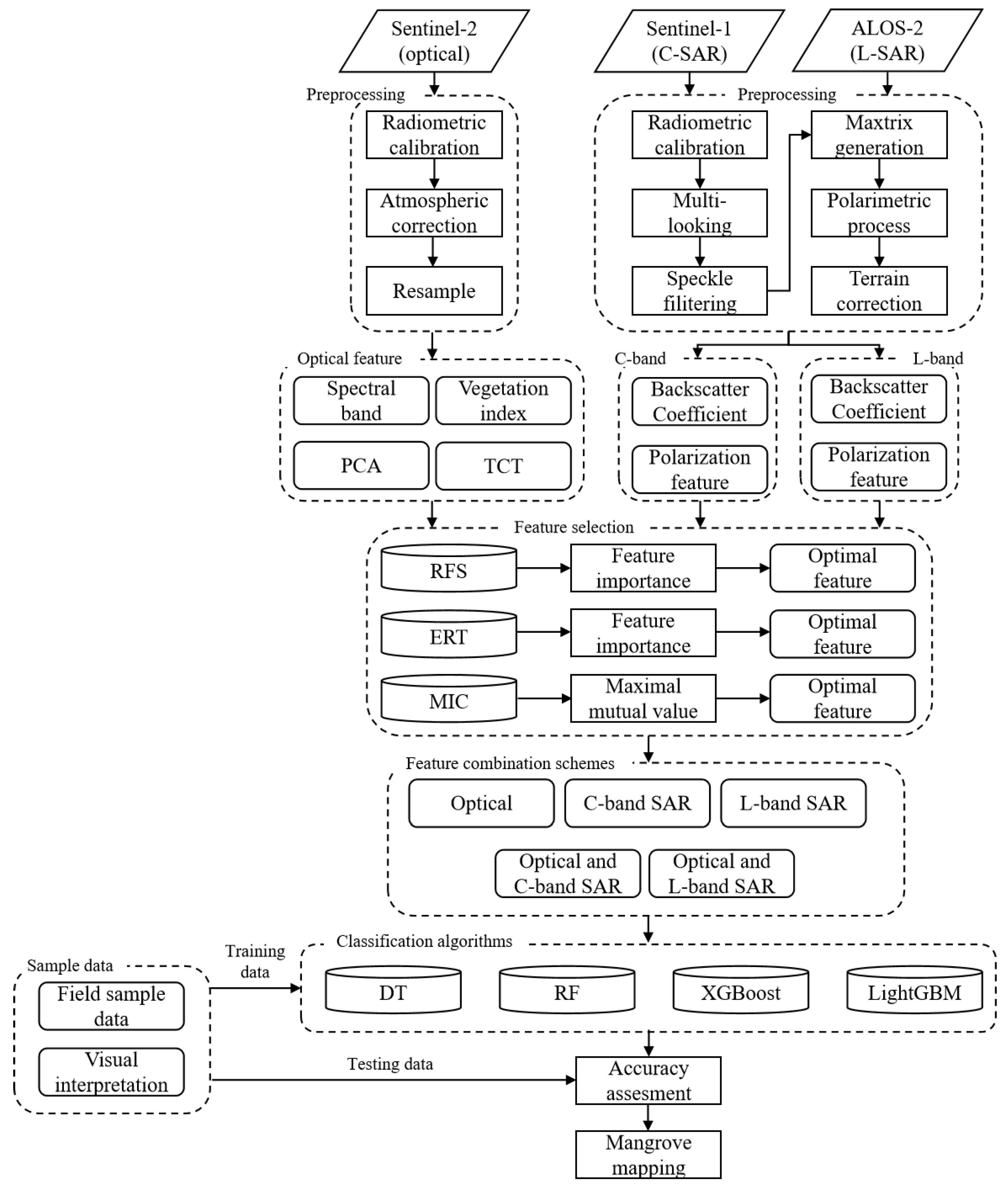
Figure 1. Workflow for mangrove extraction.
Remotesensing 15 05621 g001
Figure 2. Location of the study area; (a) location of the study area in China; (b) Location of the study area in Zhanjiang City, Guangdong Province; (c) spatial distribution of sample points and the Sentinel-2B image in the study area (R: band 4, G: band 3, B: band 2). Close-ups of 8 categories of land use (dk). The two subfigures from (d) to (k) show the same category in different regions of figure (c).
Remotesensing 15 05621 g002
Figure 3. The ranking of the importance scores and mutual information values of multispectral features for three feature selection methods, (a) the importance scores of RFS, (b) the importance scores of ERT, and (c) the mutual information value of MIC.
Remotesensing 15 05621 g003
Figure 4. The ranking of the importance scores and mutual information values of polarimetric SAR features for three feature selection methods, (a,d) the importance scores of RFS, (b,e) the importance scores of ERT, (c,f) the mutual information value of MIC.
Remotesensing 15 05621 g004
Figure 5. The overall accuracy for different data sources in this study. The red dotted line indicates an acceptable accuracy of 85%. (a) S2 optical data, (b) S1 C-band SAR data, (c) A2 L-band SAR data, (d) S2 optical and S1 SAR data, and (e) S2 optical and A2 SAR data.
Remotesensing 15 05621 g005
Figure 6. The ranking of the importance scores with combination of multispectral features and dual-polarized SAR features. (a) The importance scores with combination of S2 and S1 features; (b) the importance scores with combination of S2 and A2 features.
Remotesensing 15 05621 g006
Figure 7. Heat map for UA and PA of combining multispectral data and dual-polarized SAR data. (MG: mangrove forest, TV: terrestrial vegetation, CL: cultivated land, BL: building land, BE: culture pond, WB: water body, TF: tidal flat). (a) S2 + S1 scheme and RFS method, (b) S2 + A2 scheme and RFS method, (c) S2 + S1 scheme and ERT method, (d) S2 + A2 and ERT method, (e) S2 + S1 and MIC method, and (f) S2 + A2 scheme and MIC method.
Remotesensing 15 05621 g007
Figure 8. Classification results of the two schemes based on four machine learning algorithms. (a) SC scheme and DT method, (b) SC scheme and RF method, (c) SC scheme and XGBoost method, (d) SC scheme and LightGBM method, (e) SL scheme and DT method, (f) SL scheme and RF method, (g) SL scheme and XGBoost method, and (h) SL scheme and LightGBM method.
Remotesensing 15 05621 g008
Table 1. The advantages and disadvantages of traditional feature selection methods and classification methods.
MethodNameAdvantagesDisadvantagesReference
Feature selection
methods
Filters
  • High computational efficiency.
  • Ignores the link between features.
  • The performance of the classifiers is not considered.
[24]
Wrappers
  • Considers the effect of feature subsets on the performance of the learner.
  • Can discover interactions between subsets of features.
  • Computationally expensive and consumes time and resources.
  • Prone to overfitting.
[12]
Embedded
  • Considers the relevance of feature subsets.
  • Reduces the computational costs.
  • Selected features are more representative.
  • Can be limited by learning algorithms.
  • Parameter tuning is complex.
[25]
Classification
algorithms
MLC
  • Has a foundation in statistical theory.
  • Estimation and modeling using sample data considering the probability distributions of categories.
  • Wide applicability.
  • Real data do not satisfy normal distribution.
  • Sensitive to data noise, and classification results are unstable.
  • Requires large sample data.
[26]
SVM
  • Better classification performance when dealing with high-dimensional and complex data.
  • High generalization capacity.
  • High flexibility in choosing different kernel functions to fit different data structures.
  • High computational complexity and long training time.
  • More sensitive to the choice of parameters and kernel functions.
  • Not applicable to large-scale datasets.
[27]
DT
  • Generation rules are simple, intuitive, and easy to understand and interpret.
  • Wide applicability for classification and regression tasks.
  • Handles nonlinear relationships.
  • Easy to overfit.
  • Higher instability and sensitivity to data variations.
  • Insufficient model flexibility.
[28]
RF
  • High robustness and generation.
  • Reduction in model variance and overfitting.
  • Provides importance assessments to make models easier to interpret.
  • Easily overfitted with a small amount of data.
  • Poor adaptation to high-dimensional sparse data.
[29]
Table 2. The remote sensing data used in this study.
Satellite/SensorData Level/Data TypeTimeSpectral/PolarizationSpatial Resolution
Sentinel-2B/MSILevel-1C5 October 2018B1 (Coastal)0.433~0.453 μm60 m
B2 (Blue)0.458~0.523 μm10 m
B3 (Green)0.543~0.578 μm10 m
B4 (Red)0.650~0.680 μm10 m
B5 (RedEdge1)0.698~0.713 μm20 m
B6 (RedEdge2)0.733~0.748 μm20 m
B7 (RedEdge3)0.773~0.793 μm20 m
B8 (NIR)0.785~0.900 μm10 m
B8a (NIRNarrow)0.855~0.875 μm20 m
B9 (Water)0.935~0.955 μm60 m
B10 (Cirrus)1.360~1.390 μm60 m
B11 (SWIR1)1.565~1.655 μm20 m
B12 (SWIR2)2.100~2.280 μm20 m
Sentinel-1A/SARSLC7 October 2018VV, VH
ALOS-2/PALSAR-2SLC18 October 2018HH, HV
Table 3. The number of sample points used in this study.
ClassesNumber of Sample Points
Training SamplesValidation SamplesTotal
Mangrove forest10545150
Terrestrial vegetation10143144
Cultivated land8537122
Building land9741138
Bare land8939128
Culture pond9842140
Water body8938127
Tidal flat 361551
Table 4. Vegetation and water indices used in this study.
Vegetation and Water IndicesAcronymsFormulaReference
Normalized Difference Vegetation IndexNDVI N I R     R e d N I R   +   R e d [33]
Enhanced Vegetation IndexEVI 2.5 ( N I R     R e d N I R   +   6 R e d     7 B l u e   +   1 ) [34]
Land Surface Water IndexLSWI N I R     S W I R 1 N I R   +   S W I R 1 [35]
Optimized Soil Adjusted Vegetation IndexOSAVI N I R     R e d N I R   +   R e d   +   0.16 [36]
Difference Vegetation IndexDVI N I R     R e d [37]
Green Difference Vegetation IndexGDVI N I R     G r e e n [38]
Green Normalized Difference Vegetation IndexGNDVI N I R     G r e e n N I R   +   G r e e n [33]
Soil Adjusted Vegetation IndexSAVI 1.5 ( N I R     R e d N I R   +   R e d   +   0.5 ) [39]
Normalized Difference Water IndexNDWI G r e e n     N I R G r e e n   +   N I R [40]
Modified Normalized Difference Water IndexMNDWI G r e e n     S W I R 1 G r e e n   +   S W I R 1 [41]
Green Ratio Vegetation IndexGRVI N I R G r e e n [38]
Visible Atmospherically Resistant IndexVARI G r e e n     R e d G r e e n   +   R e d     B l u e [42]
Infrared Percentage Vegetation IndexIPVI N I R N I R   +   R e d [43]
Renormalized Difference Vegetation IndexRDVI N I R     R e d N I R   +   R e d [44]
Nonlinear Index (NLI)NLI N I R 2     R e d N I R 2   +   R e d [45]
The corresponding multispectral data bands in the formula: B l u e : B2, G r e e n : B3, R e d : B4, N I R : B8, S W I R 1 : B11.
Table 5. The polarimetric SAR features used in this study.
SAR Data/BandFeatureNameFormulaReference
Sentinel-1A/CBackscattering featuresVV/VH S V V / S V H
ALOS-2/LBackscattering featuresHH/HV S H H / S H V
Sentinel-1A/C
ALOS-2/L
Polarization decomposition featuresEntropy (H) i = 1 2 λ i λ 1   +   λ 2 l o g 2 λ i λ 1   +   λ 2 [46]
Alpha   ( α ) i = 1 2 λ i λ 1   +   λ 2 α i
Anisotropy (A) λ 1     λ 2 λ 1   +   λ 2
λ i   is real number representing the eigenvalue of the coherence matrix.
Table 6. The overall accuracy and kappa coefficient using the optical number of features selected via three feature selection methods for four ML models.
DataOverall Accuracy and Kappa Coefficient (Optimal Number of Features)
RFSERTMIC
DTRFXGBGBMDTRFXGBGBMDTRFXGBGBM
S2OA87.00%
0.850
(14)
92.67%
0.915
(10)
92.33%
0.912
(14)
92.33%
0.912
(15)
88.33%
0.866
(15)
93.00%
0.919
(13)
92.00%
0.908
(8)
91.66%
0.904
(9)
83.00%
0.804
(17)
88.33%
0.866
(14)
86.67%
0.846
(15)
86.00%
0.838
(13)
K
OM
S1OA35.33%
0.255
(3)
39.67%
0.302
(5)
36.67%
0.268
(3)
37.00%
0.272
(5)
35.67%
0.259
(3)
40.00%
0.306
(5)
37.00%
0.272
(4)
35.33%
0.254
(4)
35.67%
0.259
(3)
39.33%
0.299
(5)
37.00%
0.272
(4)
35.33%
0.253
(5)
K
OM
A2OA27.67%
0.168
(5)
30.33%
0.194
(5)
33.67%
0.235
(4)
31.33%
0.208
(3)
27.67%
0.168
(5)
30.67%
0.198
(5)
33.67%
0.235
(4)
31.33%
0.208
(3)
27.00%
0.160
(5)
30.00%
0.190
(5)
32.00%
0.215
(5)
32.00%
0.215
(4)
K
OM
XGB: XGBoost; GBM: LightGBM; OA: overall accuracy; K: kappa coefficient; OM: optimal number of features.
Table 7. The OA and kappa of classifications derived from three feature selection methods and four ML models.
DataOverall Accuracy (%) and Kappa Coefficient
RFSERTMIC
DTRFXGBGBMDTRFXGBGBMDTRFXGBGBM
S2+S188.67%93.67%95.00%93.33%90.67%94.00%94.00%94.00%84.67%89.33%91.33%90.33%
0.8690.9270.9420.9230.8920.9310.9310.9310.8230.8770.9000.889
S2+A289.67%93.00%92.33%93.33%91.00%93.33%93.00%92.67%84.33%89.33%90.67%90.67%
0.8810.9190.9120.9230.8960.9230.9190.9150.8190.8770.8920.892
XGB: XGBoost; GBM: LightGBM; OA: overall accuracy; K: kappa coefficient.
Disclaimer/Publisher’s Note: The statements, opinions and data contained in all publications are solely those of the individual author(s) and contributor(s) and not of MDPI and/or the editor(s). MDPI and/or the editor(s) disclaim responsibility for any injury to people or property resulting from any ideas, methods, instructions or products referred to in the content.