Article

Remote Sensing Inversion and Mapping of Typical Forest Stand Age in the Loess Plateau

1
State Key Laboratory of Soil Erosion and Dryland Farming on the Loess Plateau, College of Natural Resources and Environment, Northwest A&F University, Yangling 712100, China
2
Shandong Cartographic Institute, Jinan 250002, China
3
College of Geography and Environmental Sciences, Zhejiang Normal University, Jinhua 321004, China
*
Author to whom correspondence should be addressed.
Remote Sens. 2023, 15(23), 5581; https://doi.org/10.3390/rs15235581
Submission received: 28 September 2023 / Revised: 20 November 2023 / Accepted: 28 November 2023 / Published: 30 November 2023
(This article belongs to the Section Ecological Remote Sensing)

Abstract

:
The accuracy of vegetation indices (VIs) in estimating forest stand age is significantly inadequate due to insufficient consideration of the differences in the physiological functions of forest ecosystems, which limits the accuracy of carbon sink simulation. In this study, remote sensing inversion and mapping of forest stand age were carried out on the Loess Plateau under consideration of the remote sensing mechanism of VIs and the physiological function and canopy structure of the forest using multiple linear regression (MLR) and random forest (RF) models. The main conclusions are as follows: (1) The canopy reflectance of different forest stands has a significant change pattern, and the older the forest stands, the lower the NIR reflectance. The relationship between forest stands and red edge is the most significant, and r is 0.53, and the relationship between Simple Ratio Index (SR), near-infrared reflectance of vegetation (NIRv), normalized difference vegetation index (NDVI), Global Vegetation Index and forest stands is more nonlinear than linear. (2) Principal component analysis (PCA) of canopy spectral information shows that SR, NDVI and red edge (B5) could explain 98% of all spectral information. SR, NDVI and red edge (B5) were used to construct a multiple linear regression model and random forest (RF) algorithm model, and RF has high estimation accuracy (R2 = 0.63). (3) The accuracy of the model was evaluated using reference data, and it was found that the accuracy of the RF model (R2 = 0.63) was higher than that of the linear regression model (R2 = 0.61), but both models underestimated the forest stand age when the forest stand age was greater than 50a, which may be caused by the saturation of the reflectance of the old forest canopy. The RF model was used to generate the dataset of forest stand information in the Loess Plateau, and it was found that the forest is dominated by young forests (<20a), accounting for 38.26% of the forest area, and the average age of forests in the Loess Plateau is 56.1a. This study not only improves the method of forest stand age estimation, but also provides data support for vegetation construction in the Loess Plateau.

1. Introduction

The carbon source/sink conversion relationship is significantly affected by forest stand age. Young forest has higher carbon sequestration potential, while old forest has much lower carbon sequestration potential than young forest [1,2]. Currently, there are two main methods for mapping forest stand age, remote sensing monitoring and forest plot inventory. Forest plot inventory is time-consuming and laborious, and it is impossible to realize large-scale forest stand age mapping using the forest plot inventory method [3]. Remote sensing monitoring has better timeliness and heterogeneity and can be used for large-scale mapping of forest stand age [4]. Therefore, remote sensing mapping of forest stand age is necessary for carbon sink simulation in forest construction.
Methods for retrieving forest stand age by remote sensing include the vegetation index (VI) method [5], stand growth equations (SGEs) [6] and the vegetation change tracker (VCT) algorithm [7]. As an important remote sensing characteristic parameter of plants, the VI method can be used to establish a remote sensing forest stand age simulation model based on the relationship between differences in forest reflectance and forest stand age. The dynamic changes in leaf chlorophyll content (LCC) and photosynthetic characteristics during the phenological periods of plants will have an important impact on canopy spectral response patterns, in which the leaves of mature forest canopy tend to show higher near-infrared and red reflectance contrast characteristics [8]. However, the red band, the near-infrared band and their component vegetation index are the key parameters of most remote sensing models for estimating forest stand age. In terms of the inversion model, an artificial neural network (ANN) and multiple linear regression model (MLR) are selected [5,8]. Jensen et al. [9] used single-band (red, NIR and SWIR) TM data and VIs (NDVI and RVI) to construct a forest stand age inversion model using an MLR and ANN model, and the results confirmed that NIR had a strong correlation with the forest stand age (r = 0.89), but a nonlinear model can better explain the relationship between forest stand age and model parameters. Chen et al. [10] used time-series images of NDVI to estimate the age of rubber, and the average error of age was 1.53a. Chen et al. [11] established a remote sensing inversion model of forest stand age using red, NIR and SWIR, and their model showed that the relationship between the forest stand age and spectral information of a rubber stand was different at different stages; the correlation between the near-infrared band and the forest stand in October (R2 = −0.40) was much higher than that in June (R2 = 0.13). Forest structural parameters and photosynthetic parameters are the main information for retrieving forest stand age, so they must be taken into account in the selection of characteristic bands.
SGE methods are widely used to describe the relationship between forest stand variables and forest stand age [12]. Forest height is one of the widely used variables in the stand growth equations because forest height is closely related to forest stand age, especially for forest average age [13]. Many SGEs are developed by combining forest height data. Examples include the Mitscherlich equation, Gompertz equation, logistic equation, Korf equation and Richards equation [14]. Maltman et al. [15] used SGEs coupled with maps of forest structure and site index to map forest stand age. In addition to stand parameters, topographic variables (such as elevation, slope and aspect) and climatic variables (such as temperature and precipitation) also affect forest growth, and taking these effects into account can greatly improve the accuracy of forest stand age mapping. However, it is very difficult to obtain these parameters, resulting in insufficient accuracy of the SGE model.
With the development of the Landsat satellite, a large number of forest disturbance and restoration studies have been carried out using time-series Landsat data, and the results have been used to estimate forest structure parameters [16,17,18]. Fang et al. realized the spatial distribution mapping of forest stand age using Landsat data and the VCT algorithm [17]. Diao et al. [18] also used the random forest algorithm for recursive feature elimination (RFE-RF) to estimate the forest stand age in non-disturbed areas using the spectral and texture features of Landsat images. Fujiki et al. [19] extracted the forest stand age from a change detection analysis of time-series Landsat images and then established a regression model between the forest stand age and the spectrum and texture factor of WorldView-2 to estimate the age of rubber trees. Although much progress has been made in forest stand age mapping based on remote sensing methods, there are many differences in the advantages of different algorithms. Due to the limitation of time series of remote sensing observation data, the VCT algorithm can only invert the forest stand age for the previous 30 years, but it cannot invert forest stand age information from more than 30 years ago. The accuracy of the stand growth model is high, but because of the “small old trees” caused by drought in the Loess Plateau, the forest height cannot clearly reflect the forest stand age [1]. VIs are widely used in remote sensing inversion of forest stand age, but single VIs are mainly applied, and the indication of the physiological functions of the forest and the physical basis for selecting a vegetation index are neglected. As a result, the accuracy of inversion needs to be improved.
Therefore, for this study, remote sensing inversion and mapping of forest stand age in the Loess Plateau were carried out under the consideration of forest physiological function, forest structural characteristics and the physical process of remote sensing of VIs. The main objectives of this study were as follows: (1) to quantitatively describe the relationship between spectral information and forest stand age; (2) to establish a remote sensing inversion model of forest stand age with strong spatiotemporal suitability; (3) to verify accuracy and evaluate the error of remote sensing data of forest stand age in the Loess Plateau. This study could provide a guarantee for the ecological construction of the Loess Plateau.

2. Materials and Methods

2.1. Study Area

The Loess Plateau spans 640,000 km2 and is situated in the upper and middle reaches of the Yellow River (100°54′~114°33′E and 33°43′~41°16′N) (Figure 1). It has a typical temperate continental monsoon climate, which means it is both hot and rainy at the same time. There are significant zonal peculiarities in the vegetation distribution in the Loess Plateau. The Loess Plateau has the biggest loess dispersion in the world, with certain regions having loess thicknesses of over 200 m. The Loess Plateau has an inland arid and semi-arid climate, and the precipitation has obvious seasonal characteristics: the annual average precipitation is 100–800 mm, concentrated in June to September. The annual average temperature is 7 °C, showing a decreasing trend from southeast to northwest. The Chinese government has implemented a number of ecological restoration initiatives to address the region’s substantial soil erosion issues as a result of serious past ecological difficulties. Particularly, the “Gain for Green” project, which has been in place since 1999, has resulted in a notable increase in vegetation cover and efficient soil erosion control. However, in this context, the carrying capacity of the region’s water resources has reached its limit [1]. Currently, the vegetation types of the Loess Plateau are mainly artificial forest and grassland, and the forest types mainly include evergreen needle-leaf forests (ENFs), mixed forests (MFs), deciduous broadleaf forests (DBFs) and evergreen broadleaf forests (EBFs).

2.2. Data Source

2.2.1. Forest Stand Age and Forest Cover Data

Forest inventory data were used for comparing and validating forest stand age modeling and mapping. Forest inventory data come from China’s 9th National Forest Inventory (NFI) containing attributes of dominant tree species, average forest stand age, the proportion of dominant tree species, average forest height, forest density (number of plants per hectare), average diameter at breast height (DBH) and site index for each forest quadrat during 2014–2018, but they were updated to 2019 and rasterized into 30 m resolution maps using the nearest neighbor resampling method. The dominant tree species were determined by tree volume and tree density, and those with similar attributes were merged into one forest polygon. The average forest stand age and tree height of the dominant tree species within a forest polygon were taken as the final forest stand age and tree height [19,20], and the forest age data of 603 quadrats were collected in this study. A Circa 2010 Thirty Meter Resolution Forest Map for China (http://data.starcloud.pcl.ac.cn/zh) was selected. These data were produced based on the combination of forest census and Landsat data with a resolution of 30 m [21].

2.2.2. Optical Remote Sensing Data

Sentinel-2 data were downloaded from the ESA (https://scihub.copernicus.eu/dhus/#/home (accessed on 10 October 2023))). Forest canopy reflectance has significant seasonal variation patterns [22]. Due to the complexity and diversity of forest ecosystems, different forest canopy structures, plant functional traits (such as leaf structure and pigment content), water stress and forest health status all affect their spectral features, and maximum canopy reflectance is a proxy for canopy photosynthetic capacity [23,24]. Therefore, the maximum reflectance of the forest phenological period was selected as the data for remote sensing inversion. The forest leaf germination period is from late March to late April of each year, and the leaf extension period is from early May to early August of each year. The forest defoliation period is from mid-September to late October in the Loess Plateau. Sentinel-2 L2A product data were selected using Google Earth Engine (GEE) to complete the synthesis of maximum reflectance in the growing season, and the spatial resolution was resampled to 30 m, which is consistent with the spatial scale of field observation data. In this study, Google Earth Engine (GEE) was used to implement Sentinel-2 data preprocessing. The Savitzky–Golay (S-G) filtering algorithm was selected to achieve spectrum smoothing and de-noising in the growing season. We used forest cover data to inundate Sentinel data to obtain forest canopy reflectance.

2.3. Methods

In this study, forest inventory data, remote sensing data and a machine learning model were used to implement remote sensing retrieval of forest stand age information in the Loess Plateau. The main technical route is shown in Figure 2. For this study, the relationship between spectral information and forest stand age was quantitatively described, and a remote sensing inversion model of forest stand age with strong spatiotemporal suitability, supported by a machine learning algorithm, was established; this was followed by accuracy verification and error evaluation of remote sensing data of forest stand age in the Loess Plateau.

2.3.1. Selection of Vegetation Indices

For this study, normalized difference vegetation index (NDVI), Simple Ratio Index (SR), near-infrared reflectance of vegetation (NIRv) and greenness vegetation index (GVI) were selected for the retrieval of forest stand age in the Loess Plateau. Spectral changes in forest canopy at different forest stand ages can be better applied to the exploration of the relationship between vegetation indices and forest stand age. Table 1 shows the calculation formulas of each vegetation index.
NDVI is used to detect the forest vegetation growth state and forest coverage, eliminate some radiation errors and reflect the influence of canopy background (such as soil, snow, dead leaves and roughness) and vegetation cover [25,26]. SR is the ratio of light scattered in the near-infrared to light absorbed in the red band, which reduces the influence of atmosphere and topography. For the vegetation with a larger leaf area index (LAI) or higher canopy, the value is higher. For soil, water and non-vegetation elements, the value is lower [27,28]. NIRv is a canopy vegetation reflectance index calculated using NDVI and can effectively reduce the influence of soil background reflectance. NIRv has become an effective tool for studying plant photosynthesis in recent years. Studying the relationship between NIRv and gross primary productivity (GPP) on multiple time scales is of great significance for exploring GPP at global and regional scales [29,30]. GVI is the weighted sum of the radiation brightness values of each band, and the radiation brightness is the comprehensive result of atmospheric radiation, solar radiation and environmental radiation, so it is greatly affected by external conditions (such as atmosphere and soil) [31,32].

2.3.2. Exploration of Response of Canopy Spectra to Forest Stand Age

Spectral response characteristics refer to the different properties of a substance under different wavelengths of light. The absorption of light at different wavelengths is different in plant leaves, so there are absorption peaks in the spectrum [33,34]. These peaks can be used to study the photosynthesis and growth of plants. Canopy spectra observed by satellite are significantly affected by leaf spectra and canopy structure. Obviously, there are differences in spectral characteristics of forest stands of different ages due to differences in canopy structure and leaf photosynthesis. This is the basis for studying the response of spectral characteristics to forest stand age. The response of spectral characteristics to forest stand age can be quantitatively evaluated by the Pearson correlation coefficient. In this study, the Pearson correlation coefficient was used to analyze the relationship between stand age and vegetation spectral parameters, and its significance was detected using a p-value [35].

2.3.3. Inversion Model of Forest Stand Age

Accurate input parameters are the key to accurate inversion of a remote sensing model of forest age. Principal component analysis (PCA) was selected as the data for the characteristic parameters of the model; this method removes noise and unimportant features from high-dimensional spectral data and realizes the selection of model input parameters [36].
Two types of methods were chosen to map forest stand age, namely the random Forest (RF) algorithm and the multiple linear regression (MLR) model. The RF algorithm is a bagging algorithm, and a bagging algorithm is a kind of ensemble learning method. Ensemble learning is the process of training multiple weak models to form a strong model [37]. The performance of the strong model is much better than that of a single weak model. In the training phase, the random forest uses bootstrap sampling to collect multiple different sub-training datasets from the input training dataset to train multiple different decision trees in turn. In the prediction phase, the random forest averages the prediction results of multiple internal decision trees to obtain the final results [38]. The algorithm mainly considers the two processes of the training stage and the prediction stage to realize the forest stand age inversion based on remote sensing data. In the training stage, bootstrap sampling is used to collect several different sub-training datasets from the input training dataset to train several different decision trees in turn. In the prediction stage, the forest stand age inversion model is obtained by averaging the prediction results of multiple decision trees. MLR refers to a linear regression model containing multiple explanatory variables, which is used to explain the linear relationship between the explained variable and explanatory variables [39].
Using the position information of forest stand age observation sample points, we extracted the corresponding sentinel data canopy reflectance, a total of 603 pairs of spectral and corresponding age data, and divided the data into a training set (accounting for 70% of the total dataset) and verification set (accounting for 30% of the total dataset).

2.3.4. Forest Stand Age Mapping and Accuracy Assessment

Two indicators, namely the coefficient of determination (R2) and root-mean-square error (RMSE) [40], were used to compare and evaluate the accuracy of forest stand age mapping and modeling using different stand growth models and machine learning methods.
R M S E = 1 n i = 1 n ( ( y i y i ' ) 2 )
R 2 = 1 i = 1 n ( y i y i ' ) 2 i = 1 n ( y i y ¯ ) 2
where n represents the number of samples, i represents the i-th sample point, yi represents the reference forest stand age, y i ' represents the mapped forest stand age and y ¯ represents the mean value of the reference forest stand age.

3. Results

3.1. Characteristics of Spectral Changes in Different Forest Stand Ages

3.1.1. Seasonal Variation Patterns of Canopy Spectra

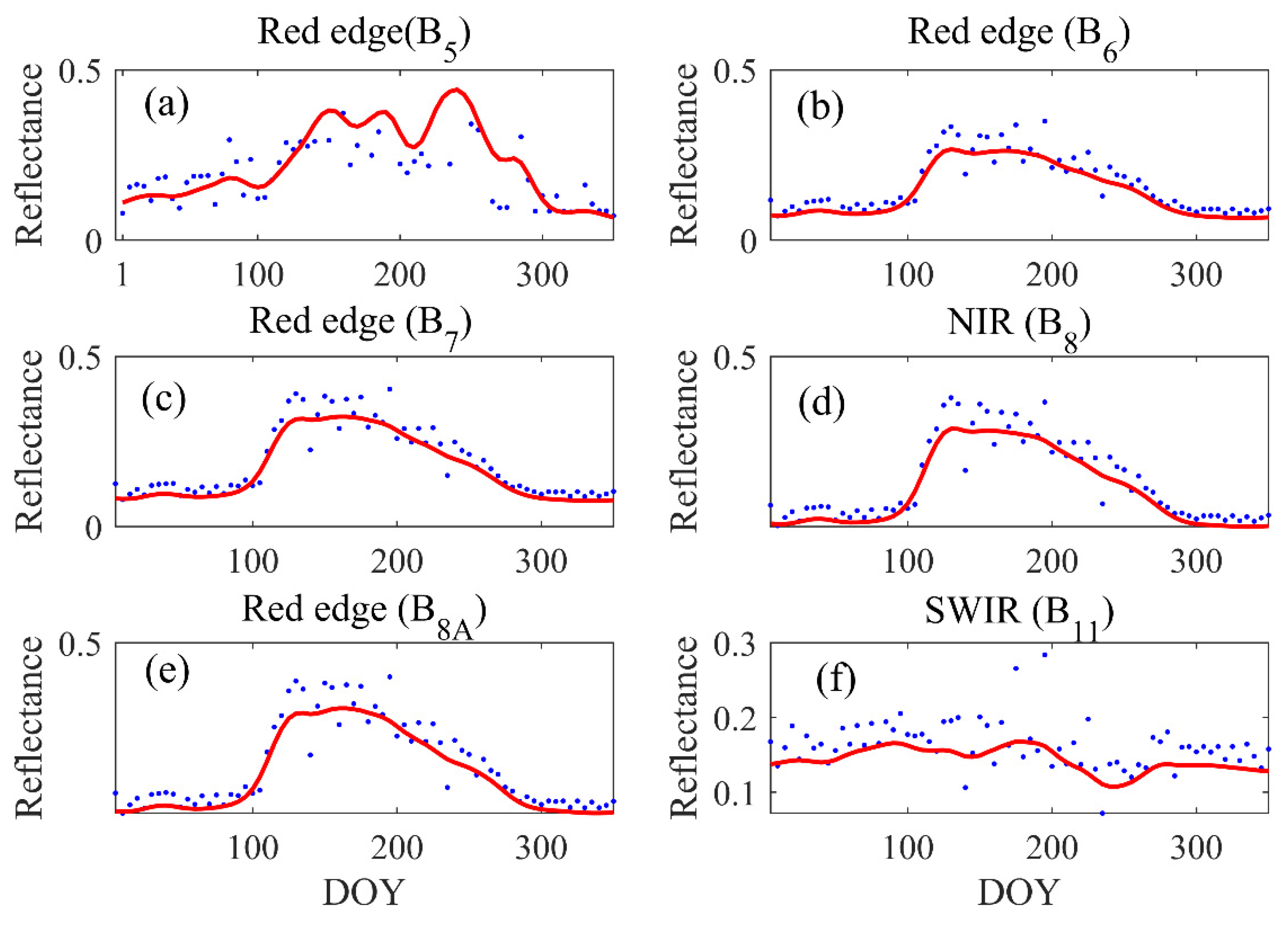
Figure 3 shows the seasonal variation patterns of vegetation red edge (B5, B6, B7 and B8A), NIR (B8) and short-wave infrared (B11) bands in Sentinel-2 data, and it is found that all bands except for the thermal infrared band (B11) have significant seasonal changes. The S-G filtering algorithm is a polynomial smoothing algorithm based on the least square principle in the time domain; it can eliminate spectral noise to the greatest extent and ensure the real information of the spectrum is obtained. The results show that the S-G algorithm could smooth the spectral data and effectively extract the development process of the forest plant canopy, especially in the red edge (B5, B6, B7 and B8A), NIR (B8) and SWIR (B11) bands of vegetation. However, the seasonal variation in the canopy B11 is weak because the canopy thermal infrared data are mainly affected by other factors such as weather.

3.1.2. Spectral Change Patterns of Different Forest Stand Ages

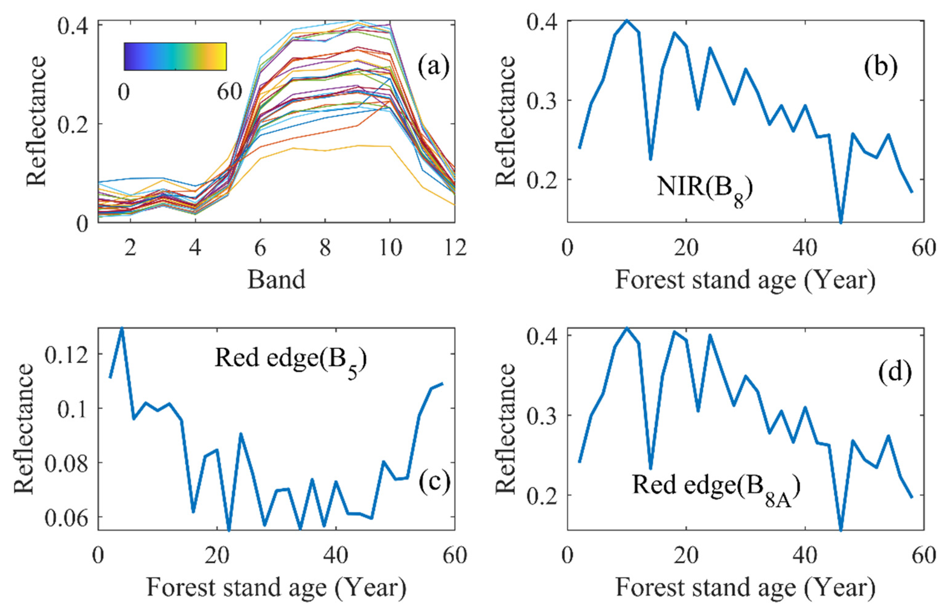
For this study, the spectral change patterns of different forest stand ages were analyzed, as shown in Figure 4. Figure 4a shows the typical spectral information of different forest stand ages, and the color of the canopy spectral curve represents the forest stand age. The forest canopy spectral curve of 1–60a was mainly selected for analysis. Figure 4b shows the trend of the change in the near-infrared (B8) reflectance value with forest stand age. The results show that with the increase in forest stand age, the near-infrared reflectance of vegetation canopy shows a significant decline trend. Figure 4c shows the trend of the change in the red edge (B5) reflectance value with forest stand age. The results show that the red edge reflectance of the vegetation canopy presents a “U-shaped” change trend with the increase in forest stand age. Figure 4d shows the trend of the variation in the red edge (B8A) reflectance value with forest stand age. It is found that with the increase in forest stand age, the red edge reflectance of the vegetation canopy shows a significant decreasing trend. Therefore, these results indicate that forest canopy spectra of different ages have significant change patterns, and they further confirm that canopy spectra can reflect forest stand age.

3.2. Relationship between Forest Stand Age and Canopy Spectral Characteristics

3.2.1. Relationship between Canopy Reflectance and Forest Stand Age

Clarifying the decoupling relationship between forest canopy spectral information and forest stand age, especially the linear or nonlinear relationship between forest stand age and canopy spectral parameters, is the basis of remote sensing inversion of stand age. In this study, the Pearson correlation coefficient was used to analyze the relationship between the reflectance of the B11 bands of remote sensing data and forest stand age, as shown in Table 2. The results show that there is a significant correlation between forest stand age and canopy spectral reflectance.
Forest stand age and canopy near-infrared (B8) spectral reflectance and red edge (B8A) reflectance were the most significant, with r values of 0.53 and 0.39, respectively. This shows that forest stand age significantly affects the spectral reflectance of the canopy. The reflectance of the canopy is a comprehensive reflection of the canopy structure and the photosynthetic capacity of forest leaves. These results indicate that the variation in canopy structure and photosynthetic capacity with forest stand age can be captured by remote sensing data.

3.2.2. Relationship between Vegetation Indices and Forest Stand Age

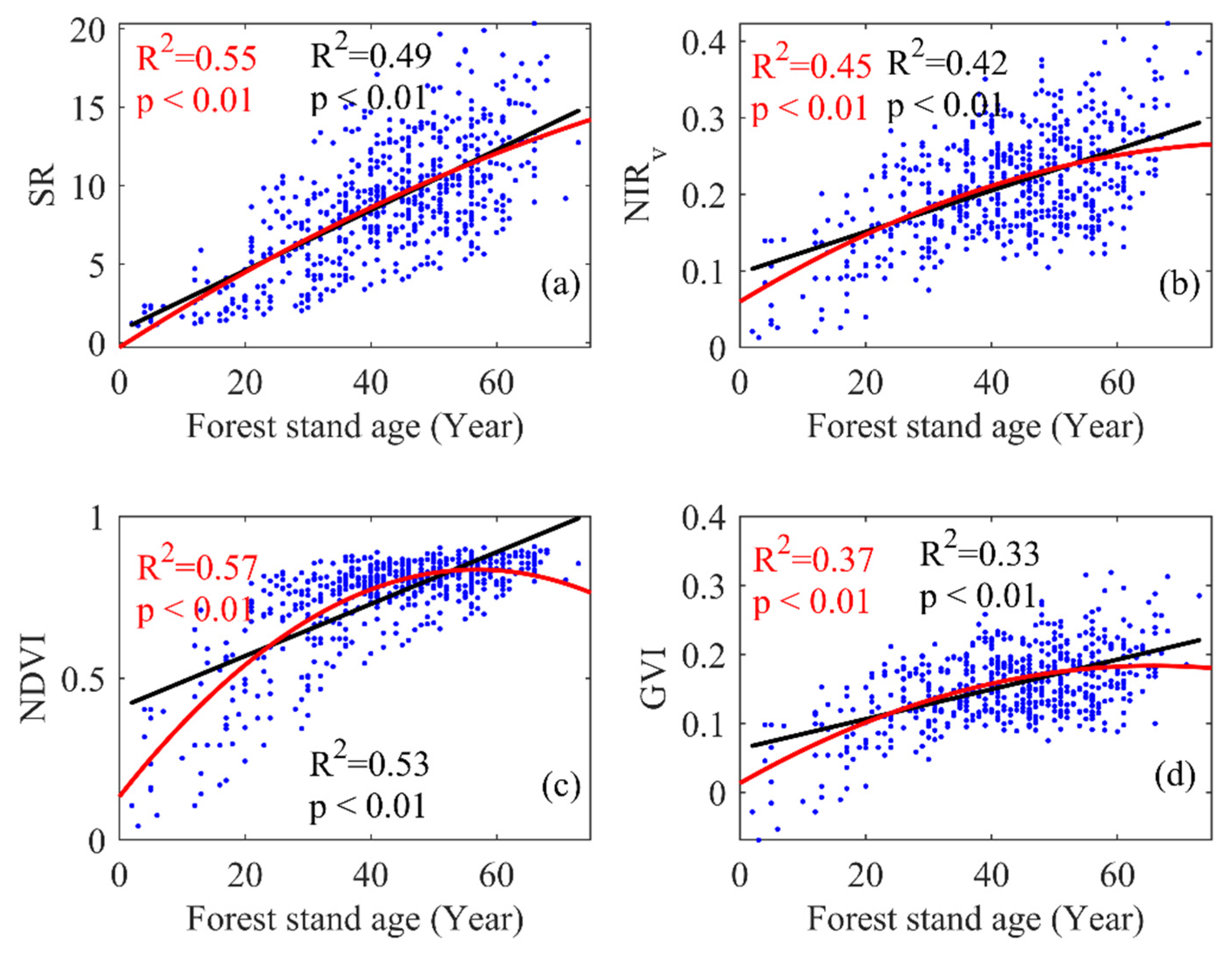
To eliminate the effects of forest background reflectance and topographic effects, vegetation indices were introduced to study the canopy spectrum and forest stand age. A vegetation index can eliminate the effects of forest background reflectance and topographic effects on the spectrum by means of band combination methods. The linear (black fitting line) and nonlinear (red fitting line) relationships between SR, NIRv, NDVI, GVI and forest stand age were analyzed, and the results are shown in Figure 5. For the relationship between SR and forest stand age, the R2 of the nonlinear relationship is 0.55, and the R2 of the linear relationship is 0.49. The nonlinear relationship is significantly higher than the linear relationship, indicating that when the forest stand age reaches the age threshold, the change in structural parameters slows down, and the nonlinear fitting curve approaches saturation. For the relationship between NIRv and forest stand age, the R2 of the nonlinear relationship is 0.45, and the R2 of the linear relationship is 0.42; in this case, the nonlinear relationship is also significantly higher than the linear relationship. Similarly, when the forest stand age reaches the age threshold, the change in photosynthetic parameters slows down, and the non-fitting line slowly approaches saturation. For the relationship between NDVI and forest stand age, the R2 of the nonlinear relationship is 0.57, and the R2 of the linear relationship is 0.53; the nonlinear relationship is significantly higher than the linear relationship. When the forest stand age is 45 years, NDVI shows a peak and a sharp decline trend. For the relationship between GVI and forest stand age, the R2 of the nonlinear relationship is 0.37, and the R2 of the linear relationship is 0.33; the nonlinear relationship is significantly higher than the linear relationship, and GVI has a saturation trend, but it is not sensitive enough.

3.3. Establish of Forest Stand Age Inversion Model in Loess Plateau

3.3.1. Spectral Feature Extraction Using PCA

There is a significant correlation between the spectral data, as shown in Figure 6. In the application of quantitative remote sensing, the representative worth band or vegetation index without duplicate information is generally selected to achieve linear or nonlinear dimensionality reduction of spectral information. In this study, the principal component analysis method (PCA) was used to reduce the dimensionality of spectral information. Figure 6 shows the covariance matrix (M) of the principal components. The grid value is the covariance between each vector element, which is a natural generalization process from a scalar random variable to a high-dimensional random vector.
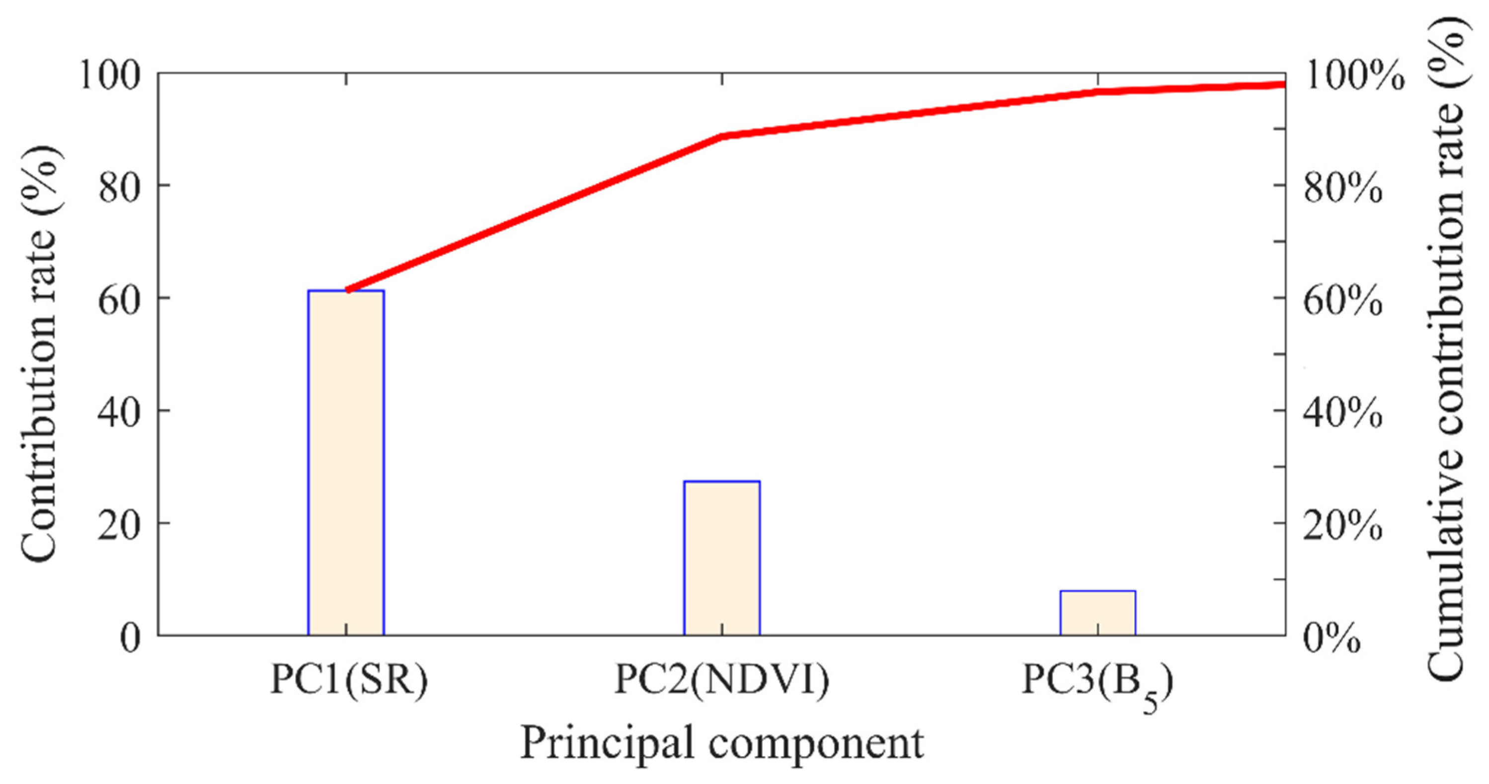
Figure 7 shows the cumulative contribution rate of the principal components of canopy spectral information. When the first three principal components are selected, namely PC1 (SR), PC2 (NDVI) and PC3 (B5), 98% of canopy spectral information can be interpreted. In particular, the structure vegetation index SR can explain 61% of the spectral information, so for forests, the structural parameters of forests are the main difference from other features. PC2 (NDVI), which quantifies forest photosynthesis and forest greenness by the difference between near-infrared (strong leaf reflection) and red light (leaf absorption), provides 30% of the spectral information. PC3 (B5) is able to interpret 9% of the spectral information. Therefore, the three principal components were used in the estimation of forest stand age in the Loess Plateau.

3.3.2. Establishment of Forest Stand Age Inversion Model Using MLR Model

In this study, a multiple nonlinear regression model was selected to establish a remote sensing inversion model of forest stand age in the Loess Plateau. About 70% of the data (400 pairs of data) were selected as regression samples, and the remaining samples were used for dataset validation. The model structure of Age = a × SR + b × NDVI + c × B5 + d (a, b, c and d were unknown parameters) was constructed using MATLAB 2023a, and the optimal solution of its parameters was obtained by using the partial least square method. The results are shown in Table 3. This model has high accuracy, and its R2 is 0.69.

3.3.3. Establishment of Forest Stand Age Inversion Model Using RF Model

The regression random forest model mainly considered the two processes of the training stage and the prediction stage to realize the forest stand age inversion based on remote sensing data. In MATLAB 2023a, 603 pairs of data were randomly divided into two datasets; about 70% (400 pairs of data) were used as regression samples, and the remaining samples were used for dataset validation. The model was trained 30 times, and the model with the largest R2 was selected; the maximum R2 was 0.63.

3.4. Comparison of Accuracy of Remote Sensing Inversion Models for Forest Stand Age

In this study, 30% (203 pairs of data) of data were selected as reference data to verify the dataset of forest stand age retrieved by remote sensing methods. The relationship between reference forest stand age data and remote sensing simulated forest stand age is shown in Figure 8. Figure 8a shows that the relationship between reference data and forest stand age simulated by the MLR model is very significant; the R2 is 0.61, the slope of the fitting line is 1.12 and the root-mean-square error (RMSE) is 10.98. We found that the model underestimated the forest stand age when the forest stand age was greater than 50. The main reason is that the vegetation index has different saturation effects with the increase in age, but the linear regression model cannot better eliminate the saturation effect of the VI when estimating forest stand age. Also, Figure 8b shows that the relationship between the reference age and forest stand age simulated by the RF model is very significant; the R2 is 0.63, the slope of the fitting line is 1.09 and the RMSE is 10.77. Although the model also underestimated the forest stand age when the forest stand age was greater than 50, compared with the MLR model, the error of the RF model was weakened, and the slope decreased from 1.12 to 1.09. In short, although the machine learning model is a “black box” model, it solves fitting problems such as data collinearity and improves the regression accuracy of the model.

3.5. Spatial Distribution of Forest Stand Age in Loess Plateau

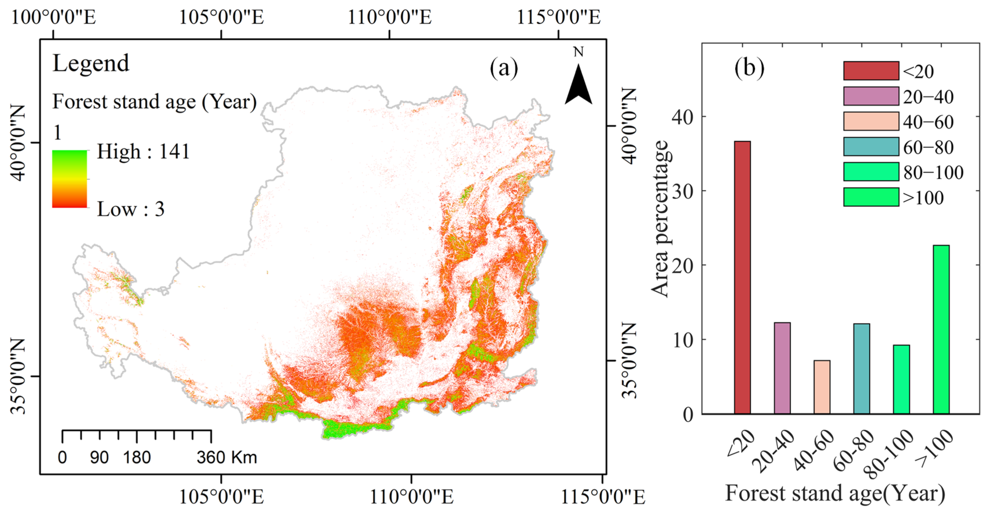
Figure 9 shows the spatial distribution map of forest stand age in the Loess Plateau produced using the RF model. The results showed that the age distribution of <20 years old and 20–40 years old accounted for 38.26% and 12.22%, respectively. Forests older than 100 years reached 24.01%, mainly distributed in the east and south of the Loess Plateau. The forests in the Loess Plateau are mainly young forests. Due to severe soil erosion problems in the region, the Chinese government initiated reforestation campaigns in the 1970s and implemented the largest historical afforestation project called “Gain for Green” in 1999 [1], which explains why the stand age distribution map has a higher proportion of young forests and verifies the validity of our results.

4. Discussion

4.1. Accuracy Evaluation and Uncertainty Analysis of Inversion Models

We verified the model with reference data, and the accuracy of the model is high. However, we found that with the increase in forest stand age, different vegetation indices showed a saturation effect. This study established a remote sensing inversion model of forest stand age in the Loess Plateau and realized the mapping of forest stand age used in the remote sensing process considering the physiological function and canopy structure of the forest ecosystem. The accuracy of the model is reliable, but there are some defects. Although clouds and shadows are removed from the input data of the inversion model, there are some differences in the seasons, and the error transmission of the data will aggravate the uncertainty of the remote sensing dataset of forest stand age information in the Loess Plateau.
Cloud cover in optical remote sensing images will obscure the ground information to different degrees, which causes the blurring and missing of the surface observation information and greatly affects the imaging quality of remote sensing images, significantly reducing the accuracy of a quantitative remote sensing model [41]. To avoid the impact of cloud coverage on the accuracy of the model, Sentinel-2’s new cloud removal method (S2cloudless algorithm) was used. The S2cloudless algorithm is a machine learning algorithm through which cloud mask files can be calculated for Sentinel-2 images [42]. Tarasov compared the cloud removal accuracy of the traditional Fmask and Sen2Cor algorithms and the machine-learning-based S2cloudless algorithm and found that S2cloudless showed the best result (average accuracy 83%), and the lowest accuracy was obtained with Fmask (70%). The seasonal variability in cloud masking accuracy did not exceed 6% [43]. Therefore, we reduced the impact of cloud inversion on the accuracy of the model and used the S2cloudless algorithm to improve the accuracy of the model.

4.2. Spatial Inconsistency between the Observed Sample and Remote Sensing Data Significantly Affects the Accuracy of the Model

The scale inconsistencies of the observed plots also significantly affect the accuracy of the model; observational data are mainly from China’s Ninth National Forest Inventory (NFI), which includes various forest quadrats from 2014 to 2018, but these data have been updated to 2019 by rasterization into a 30 m resolution map using the nearest neighbor resampling method [19,20]. Although the average age and height of the dominant tree species within a forest polygon were used as the final age and height of the forest, the scale of the observed quadrangle would cause errors. At the same time, the spatial matching between satellite image pixel size and observation quadrats also significantly affects the accuracy of the model, but these errors are unavoidable.

4.3. Background Reflectance Affects the Accuracy of Model

A forest has a complex hierarchical structure in the vertical direction. Temperate forests have two vertical layers: a forest canopy composed mainly of trees and understory vegetation composed mainly of shrubs, herbs and mosses [43]. The reflected signals received by the sensor come not only from the forest canopy, but also from the background features under the forest canopy [44]. The results show that forest background reflectance has significant spatiotemporal variation, and the spatiotemporal variation in background reflectance is usually ignored in forest parameter inversion studies based on remote sensing data, resulting in significant error of the inversion model, and the error of the inversion model is larger when the forest canopy is low [45,46]. As shown in Figure 8, the reason for the deviation between the simulated forest stand age and the reference forest stand age of young forest and old forest may be directly related to the background reflectance. The canopy of young forest is small, the coverage is insufficient and the pixel reflectance mainly comes from the forest background [47]. As a result, the model overestimates young forest stand age. From the perspective of the inversion of forest canopy parameters, the impact of forest background reflectance cannot be ignored. In a sparse forest area, the difference in forest background reflectance leads to a great difference in canopy reflectance [48]. It was observed that the total reflectance of the same forest area when the background reflectance is high is much larger than that when the background reflectance is low under the same forest period in the direction of substellar points in the red wavelength band [49].
Therefore, the inversion of forest parameters by ignoring forest background reflectance leads to significant errors in the model. SR is the ratio of light scattered in the near-infrared to light absorbed in the red band, which reduces the influence of atmosphere and topography [27,28]. So, background reflectivity is one of the key parameters for establishing a remote sensing estimation model of forest parameters.

5. Conclusions

The accuracy of vegetation indices in estimating forest stand age is significantly inadequate due to insufficient consideration of the differences in the physiological functions of forest ecosystems. In this study, remote sensing inversion and mapping of forest stand age in the Loess Plateau were carried out under consideration of the mechanism of the remote sensing of vegetation indices and the physiological function and canopy structure of the forest. The main conclusions are as follows:
(1)
The canopy reflectance of different forest stand ages has a significant change pattern, and the older the forest stands, the lower the NIR reflectance; the relationships between SR, NIRv, NDVI, GVI and forest stand age were more nonlinear than linear.
(2)
Principal component analysis (PCA) of canopy spectral information showed that SR, NDVI and red edge (B5) could explain 98% of all spectral information. SR, NDVI and B5 were used to construct MLR and RF models, and the RF model was found to have high estimation accuracy (R2 = 0.63).
(3)
The accuracy of the models was evaluated using reference data, and it was found that the accuracy of the RF model (R2 = 0.63) was higher than that of the MLR model (R2 = 0.61), but both models underestimated the forest stand age when the forest stand age was greater than 50a, which may be caused by the saturation of the reflectance of the old forest canopy. The RF model was used to generate a dataset of forest stand age, and it was found that the forest is dominated by young forests (<20a), accounting for 38.26% of the forest area. This study not only improves the method of forest stand age estimation, but also provides data support for vegetation construction in the Loess Plateau, which are the key data for carbon sink simulation of the regional ecosystem.

Author Contributions

Conceptualization, X.W. and J.S.; methodology, X.W.; software, J.S., C.G. and C.W.; writing—original draft preparation, X.W.; writing—review and editing, F.Z. All authors have read and agreed to the published version of the manuscript.

Funding

This research was funded by the China Postdoctoral Science Foundation, grant number 2023M732873; Fundamental Research Funds for Central Universities, grant number 2452022125; and National Natural Science Foundation of China, grant number 42207396.

Data Availability Statement

The Sentinel-2 dataset for the period from January 2019 to December 2019 can be downloaded at https://scihub.copernicus.eu/dhus/#/home (accessed on 10 October 2023).

Acknowledgments

The authors thank the anonymous reviewers and editors for their work.

Conflicts of Interest

The authors declare no conflict of interest.

References

  1. Feng, X.; Fu, B.; Piao, S.; Wang, S.; Ciais, P.; Zeng, Z.; Lü, Y.; Zeng, Y.; Li, Y.; Jiang, X.; et al. Revegetation in China’s Loess Plateau is approaching sustainable water resource limits. Nat. Clim. Change 2016, 6, 1019–1022. [Google Scholar] [CrossRef]
  2. Baishya, R.; Barik, S. Estimation of tree biomass, carbon pool and net primary production of an old-growth Pinus kesiya Royle ex. Gordon forest in north-eastern India. Ann. For. Sci. 2021, 68, 727–736. [Google Scholar] [CrossRef]
  3. Li, W.; Niu, Z.; Shang, R.; Qin, Y.; Chen, H. High-resolution mapping of forest canopy height using machine learning by coupling icesat-2 lidar with sentinel-1, sentinel-2 and landsat-8 data. Int. J. Appl. Earth Obs. Geoinf. 2020, 92, 102163. [Google Scholar] [CrossRef]
  4. Zhang, Y.; Yao, Y.; Wang, X.; Liu, Y.; Piao, S. Mapping spatial distribution of forest age in China. Earth Space Sci. 2017, 4, 108–116. [Google Scholar] [CrossRef]
  5. Tang, S.; Tian, Q.; Xu, K.; Xu, N.; Yue, J. Age information retrieval of Larix gmelinii forest using Sentinel-2 data. Natl. Remote Sens. Bull. 2020, 24, 1511–1524. [Google Scholar] [CrossRef]
  6. Yu, Z.; Zhao, H.; Liu, S.; Zhou, G.; Fang, J.; Yu, G.; Tang, X.; Wang, W.; Yan, J.; Wang, G.; et al. Mapping forest type and age in China’s plantations. Sci. Total Environ. 2020, 744, 140790. [Google Scholar] [CrossRef] [PubMed]
  7. Chen, B.; Jin, Y.F.; Brown, P. Automatic mapping of planting year for tree crops with Landsat satellite to time series stacks. ISPRS J. Photogramm. Remote Sens. 2019, 151, 176–188. [Google Scholar] [CrossRef]
  8. Grant, L. Diffuse and specular characteristics of leaf reflectance. Remote Sens. Environ. 1987, 22, 309–322. [Google Scholar] [CrossRef]
  9. Jensen, J.R.; Qiu, F.; Ji, M.H. Predictive modelling of coniferous forest age using statistical and artificial neural network approaches applied to remote sensor data. Int. J. Remote Sens. 1999, 20, 2805–2822. [Google Scholar]
  10. Chen, G.; Thill, J.C.; Anantsuksomsri, S.; Tontisirin, N.; Tao, R. Stand age estimation of rubber (Hevea brasiliensis) plantations using an integrated pixel-and object-based tree growth model and annual Landsat time series. ISPRS J. Photogramm. Remote Sens. 2018, 144, 94–104. [Google Scholar] [CrossRef]
  11. Chen, B.Q.; Cao, J.H.; Wang, J.K.; Wu, Z.X.; Tao, Z.L.; Chen, J.M.; Yang, C.; Xie, G.S. Estimation of rubber stand age in typhoon and chilling injury afflicted area with Landsat TM data: A case study in Hainan Island, China. For. Ecol. Manag. 2012, 274, 222–230. [Google Scholar] [CrossRef]
  12. Gadow, K.V.; Hui, G. Modelling Forest development. For. Sci. 1999, 57, 1146–1158. [Google Scholar]
  13. Sharma, M.; Parton, J. Height-diameter equations for boreal tree species in Ontario using a mixed-effects modeling approach. For. Ecol. Manag. 2007, 249, 187–198. [Google Scholar] [CrossRef]
  14. Lin, X.; Shang, R.; Chen, J.M.; Zhao, G.; Zhang, X.; Huang, Y.; Yu, G.; He, N.; Xu, L.; Jiao, W. High-resolution forest age mapping based on forest height maps derived from GEDI and ICESat-2 space-borne lidar data. Agric. For. Meteorol. 2023, 339, 109592. [Google Scholar] [CrossRef]
  15. Maltman, J.C.; Hermosilla, T.; Wulder, M.A.; Coops, N.C.; White, J.C. Estimating and mapping forest age across Canadas forested ecosystems. Remote Sensing. Environ. 2023, 290, 113529. [Google Scholar] [CrossRef]
  16. Huang, C.; Goward, S.N.; Schleeweis, K.; Thomas, N.; Masek, J.G.; Zhu, Z. Dynamics of national forests assessed using the Landsat record: Case studies in eastern United States. Remote Sens. Environ. 2009, 113, 1430–1442. [Google Scholar] [CrossRef]
  17. Fang, L.; Zhang, W.Q.; Yang, J.; Zhang, W.D.; Yan, Y.; Yan, Q.L. Reconstruction of stand-replacement disturbance and stand age of Chinese fir plantation based on a Landsat time series in Huitong County, Hunan. Chin. J. Ecol. 2018, 37, 3467. [Google Scholar]
  18. Diao, J.; Feng, T.; Li, M.; Zhu, Z.; Liu, J.; Biging, G.; Zheng, G.; Shen, W.; Wang, H.; Wang, J.; et al. Use of vegetation change tracker, spatial analysis, and random forest regression to assess the evolution of plantation stand age in Southeast China. Ann. For. Sci. 2020, 77, 27. [Google Scholar] [CrossRef]
  19. Fujiki, S.; Okada, K.I.; Nishio, S.; Kitayama, K. Estimation of the stand ages of tropical secondary forests after shifting cultivation based on the combination of WorldView-2 and time-series Landsat images. ISPRS J. Photogramm. Remote Sens. 2016, 119, 280–293. [Google Scholar] [CrossRef]
  20. Guo, Q.; Ren, H. Productivity as related to diversity and age in planted versus natural forests. Glob. Ecol. Biogeogr. 2014, 23, 1461–1471. [Google Scholar] [CrossRef]
  21. Li, C.; Wang, J.; Hu, L.; Yu, L.; Clinton, N.; Huang, H.; Yang, J.; Gong, P. A Circa 2010 Thirty Meter Resolution Forest Map for China. Remote Sens. 2014, 6, 5325–5343. [Google Scholar] [CrossRef]
  22. Asner, G.P.; Martin, R.E.; Anderson, C.B.; Knapp, D.E. Quantifying forest canopy traits: Imaging spectroscopy versus field survey. Remote Sens. Environ. 2015, 158, 15–27. [Google Scholar] [CrossRef]
  23. Kokaly, R.F.; Asner, G.P.; Ollinger, S.V.; Martin, M.E.; Wessman, C.A. Characterizing canopy biochemistry from imaging spectroscopy and its application to ecosystem studies. Remote Sens. Environ. 2009, 113, S78–S91. [Google Scholar] [CrossRef]
  24. Asner, G.P. Biophysical and biochemical sources of variability in canopy reflectance. Remote Sens. Environ. 1998, 64, 234–253. [Google Scholar] [CrossRef]
  25. Huang, S.; Tang, L.; Hupy, J.P.; Wang, Y.; Shao, G. A commentary review on the use of normalized difference vegetation index (NDVI) in the era of popular remote sensing. J. For. Res. 2021, 32, 1–6. [Google Scholar] [CrossRef]
  26. Pettorelli, N.; Ryan, S.; Mueller, T.; Bunnefeld, N.; Jędrzejewska, B.; Lima, M.; Kausrud, K. The Normalized Difference Vegetation Index (NDVI): Unforeseen successes in animal ecology. Clim. Res. 2011, 46, 15–27. [Google Scholar] [CrossRef]
  27. Chen, J.M. Evaluation of vegetation indices and a modified simple ratio for boreal applications. Can. J. Remote Sens. 1996, 22, 229–242. [Google Scholar] [CrossRef]
  28. Brown, L.; Chen, J.M.; Leblanc, S.G.; Cihlar, J. A shortwave infrared modification to the simple ratio for LAI retrieval in boreal forests: An image and model analysis. Remote Sens. Environ. 2000, 71, 16–25. [Google Scholar] [CrossRef]
  29. Zeng, Y.; Hao, D.; Badgley, G.; Damm, A.; Rascher, U.; Ryu, Y.; Johnson, J.; Krieger, V.; Wu, S.; Qiu, H.; et al. Estimating near-infrared reflectance of vegetation from hyperspectral data. Remote Sens. Environ. 2021, 267, 112723. [Google Scholar] [CrossRef]
  30. Badgley, G.; Field, C.B.; Berry, J.A. Canopy near-infrared reflectance and terrestrial photosynthesis. Sci. Adv. 2017, 3, e1602244. [Google Scholar] [CrossRef]
  31. Huete, A.R.; Jackson, R.D.; Post, D.F. Spectral response of a plant canopy with different soil backgrounds. Remote Sens. Environ. 1985, 17, 37–53. [Google Scholar] [CrossRef]
  32. Panda, S.S.; Ames, D.P.; Suranjan, P. Application of Vegetation Indices for Agricultural Crop Yield Prediction Using Neural Network Techniques. Remote Sens. 2010, 2, 673–696. [Google Scholar] [CrossRef]
  33. Wu, X.; Jiang, X.; Liu, H.; Allen, C.; Li, X.; Wamg, P.; Li, Z.; Yang, Y.; Zhang, S.; Shi, F.; et al. CPSDv0: A forest stand structure database for plantation forests in China. Big Earth Data 2023, 7, 222–240. [Google Scholar] [CrossRef]
  34. Wang, X.; Zhang, F.; Kung, H.; Yu, H. Spectral response characteristics and identification of typical plant species in Ebinur lake wetland national nature reserve (ELWNNR) under a water and salinity gradient. Ecol. Indic. 2017, 81, 222–234. [Google Scholar]
  35. Eggers, J.J.; Bauml, R.; Tzschoppe, R.; Girod, B. Scalar costa scheme for information embedding. IEEE Trans. Signal Process. 2003, 51, 1003–1019. [Google Scholar] [CrossRef]
  36. Liu, L.; Song, B.; Zhang, S.; Liu, X. A Novel Principal Component Analysis Method for the Reconstruction of Leaf Reflectance Spectra and Retrieval of Leaf Biochemical Contents. Remote Sens. 2017, 9, 1113. [Google Scholar] [CrossRef]
  37. Galar, M.; Fernandez, A.; Barrenechea, E.; Bustince, H.; Herrera, F. A review on ensembles for the class imbalance problem: Bagging-, boosting-, and hybrid-based approaches. IEEE Trans. Syst. Man Cybern. Part C (Appl. Rev.) 2011, 42, 463–484. [Google Scholar] [CrossRef]
  38. Fawagreh, K.; Gaber, M.M.; Elyan, E. Random forests: From early developments to recent advancements. Syst. Sci. Control Eng. Open Access J. 2014, 2, 602–609. [Google Scholar] [CrossRef]
  39. Marill, K.A. Advanced statistics: Linear regression, part II: Multiple linear regression. Acad. Emerg. Med. 2004, 11, 94–102. [Google Scholar] [CrossRef] [PubMed]
  40. Wang, X.; Zhang, F.; Ding, J.; Kung, H.T.; Latif, A.; Johnson, V.C. Estimation of soil salt content (ssc) in the ebinur lake wetland national nature reserve (elwnnr), northwest china, based on a bootstrap-bp neural network model and optimal spectral indices. Sci. Total Environ. 2018, 615, 918. [Google Scholar] [CrossRef]
  41. Zou, Z.; Shi, Z. Ship detection in spaceborne optical image with SVD networks. IEEE Trans. Geosci. Remote Sens. 2016, 54, 5832–5845. [Google Scholar] [CrossRef]
  42. Sanchez, A.H.; Picoli, M.C.A.; Camara, G.; Andrade, P.R.; Chaves, M.E.D.; Lechler, S.; Soares, A.R.; Marujo, R.F.B.; Simões, R.E.O.; Ferreira, K.R.; et al. Comparison of Cloud cover detection algorithms on sentinel–2 images of the amazon tropical forest. Remote Sens. 2020, 12, 1284. [Google Scholar] [CrossRef]
  43. Tarasov, A.V. Estimation of the accuracy of cloud masking algorithms using Sentinel-2 and PlanetScope data. Mod. Probl. Remote Sens. Earth Space 2020, 17, 26–38. [Google Scholar] [CrossRef]
  44. Spanner, M.A.; Pierce, L.L.; Peterson, D.L.; Running, S.W. Remote sensing of temperate coniferous forest leaf area index. The influence of canopy closure, understory vegetation and background reflectance. Int. J. Remote Sens. 1990, 11, 95–111. [Google Scholar] [CrossRef]
  45. Garrigues, S.; Lacaze, R.; Baret, F.; Morisette, J.T.; Weiss, M.; Nickeson, J.E.; Fernandes, R.; Plummer, S.; Shabanov, N.V.; Myneni, R.B.; et al. Validation and intercomparison of global Leaf Area Index products derived from remote sensing data. J. Geophys. Res. Biogeosci. 2008, 113, G02028. [Google Scholar] [CrossRef]
  46. Houghton, R.A. Aboveground forest biomass and the global carbon balance. Glob. Change Biol. 2005, 11, 945–958. [Google Scholar] [CrossRef]
  47. Chen, J.M.; Cihlar, J. Retrieving leaf area index for boreal conifer forests using Landsat TM images. Remote Sens. Environ. 1996, 55, 153–162. [Google Scholar] [CrossRef]
  48. Chen, J.M.; Leblanc, S. A 4-scale bidirectional reflection model based on canopy architecture. IEEE Trans. Geosci. Remote Sens. 1997, 35, 1316–1337. [Google Scholar] [CrossRef]
  49. Pisek, J.; Chen, J.M. Mapping Forest Background Reflectivity over North America with Multi-angle Imaging SpectroRadiometer(MISR)Data. Remote Sens. Environ. 2009, 113, 2412–2423. [Google Scholar] [CrossRef]
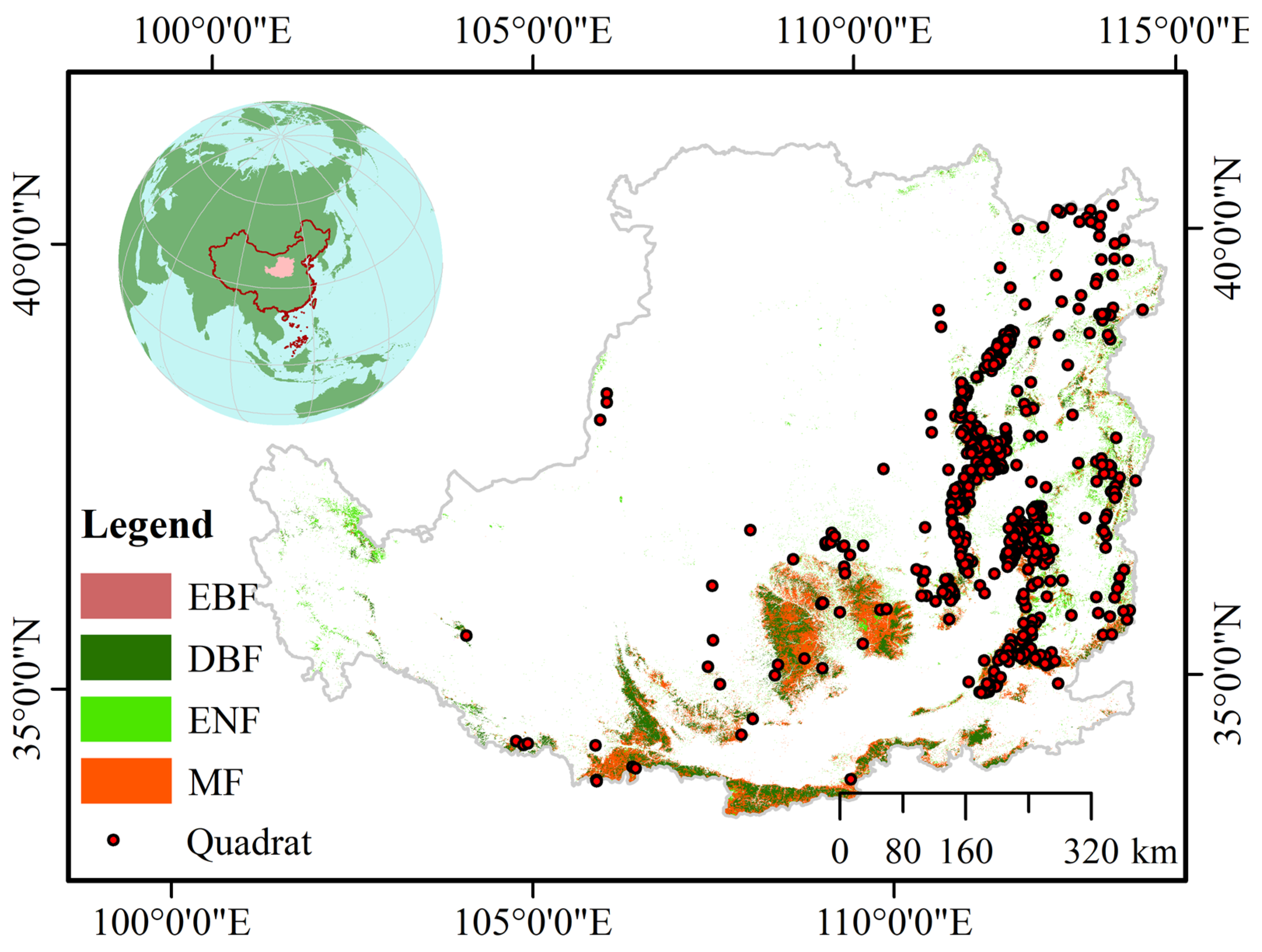
Figure 1. Forest types and spatial distribution in the Loess Plateau (evergreen needle-leaf forest (ENF), mixed forest (MF), deciduous broadleaf forest (DBF), evergreen broadleaf forest (EBF)) (forest cover data from https://data-starcloud.pcl.ac.cn/zh/resource/15 (accessed on 10 October 2023)).
Remotesensing 15 05581 g001
Figure 2. Flow chart in this study (quantitatively describe the relationship between spectral information and forest stand age and establish a remote sensing inversion model of forest stand age with strong spatiotemporal suitability; then, verify accuracy and evaluate the error of remote sensing data of forest stand age).
Remotesensing 15 05581 g002
Figure 3. Seasonal variation patterns of canopy spectra (the blue dots represent the reflectance of Sentinel data during the year, and the red lines are fitted curves). ((a) represents the seasonal pattern of Red edge(B5), (b) represents the seasonal pattern of Red edge(B6), (c) represents the seasonal pattern of Red edge(B7), (d) represents the seasonal pattern of NIR(B8), (e) represents the seasonal pattern of Red edge(B8A), (f) represents the seasonal pattern of NIR(B11)).
Remotesensing 15 05581 g003
Figure 4. Spectral reflectance characteristics of forest canopy at different ages ((a) spectral characteristics at different forest stand ages, (b) variation pattern of NIR with forest stand age, (c) variation pattern of red edge (B5) with forest stand age, (d) variation pattern of red edge (B8A) with forest stand age).
Remotesensing 15 05581 g004
Figure 5. Relationships between vegetation indices and forest stand age (the black line is the linear relationship between vegetation index and forest age, and the red line is the nonlinear relationship between vegetation index and forest age). ((a) is a scatter plot of the relationship between SR and forest stand age, (b) is a scatter plot of the relationship between NIRv and forest stand age, (c) is a scatter plot of the relationship between NDVI and forest stand age, (d) is a scatter plot of the relationship between GVI and forest stand age).
Remotesensing 15 05581 g005
Figure 6. Principal component covariance matrix (M) of canopy spectral information.
Remotesensing 15 05581 g006
Figure 7. Cumulative contribution rate of principal components of canopy spectral information.
Remotesensing 15 05581 g007
Figure 8. Accuracy evaluation of forest stand age dataset from the Loess Plateau ((a) multiple linear regression algorithm; (b) random forest algorithm) (the gray dashed line is the 1:1 line, and the red line is the fitting line).
Remotesensing 15 05581 g008
Figure 9. Spatial distribution of forest stand age in the Loess Plateau ((a) spatial distribution of forest stand age; (b) frequency of forest area at different forest stand ages).
Remotesensing 15 05581 g009
Table 1. Vegetation indices selected in this study.
Vegetation IndexEquationReferences
Normalized difference vegetation index (NDVI) N D V I = N I R R N I R + R [25,26]
Near-infrared reflectance of vegetation (NIRv) N I R v = N D V I × N I R [29,30]
Simple Ratio Index (SR) S R = N I R R [27,28]
Greenness vegetation index (GVI) G V I = 0.2941 × B 0.234 × G 0.5424 × R + 0.7276 × N I R + 0.0713 × S W I R 1 0.1608 × S W I R 2 [31,32]
Notes: NIR is the near-infrared band, R is the red band, B is the blue band, G is the green band, B is the blue band and SWIR is the short-wave infrared band.
Table 2. Pearson’s correlation coefficient for the relationship between maximum canopy reflectance and forest stand age in the growing season.
ReflectanceB1B2B3B4B5B6B7B8B8AB11B12
r0.19 *0.37 **0.35 **0.38 **0.24 **0.24 **0.39 **0.53 **0.53 **0.19 *0.21 **
** the significance level of 0.01; * the significance level of 0.05.
Table 3. Multiple linear regression model and parameters.
Input ParametersModelR2p
SR, NDVI, B5Age = 12.03 × SR + 13.25 × NDVI + 26.19 × B5 + 20.69p < 0.001
Disclaimer/Publisher’s Note: The statements, opinions and data contained in all publications are solely those of the individual author(s) and contributor(s) and not of MDPI and/or the editor(s). MDPI and/or the editor(s) disclaim responsibility for any injury to people or property resulting from any ideas, methods, instructions or products referred to in the content.