An Unsupervised Band Selection Method via Contrastive Learning for Hyperspectral Images

Abstract

Band selection (BS) is an efficacious approach to reduce hyperspectral information redundancy while preserving the physical meaning of hyperspectral images (HSIs). Recently, deep learning-based BS methods have received widespread interest due to their ability to model the nonlinear relationship between bands, with existing methods typically relying on generative algorithms. However, the process of generating images with pixel-level detail required by generative algorithm-based BS methods is computationally expensive. To alleviate this issue, we propose a contrastive learning-based unsupervised BS architecture, termed ContrastBS, in this article. With the help of contrastive learning, the proposed architecture avoids the costly generation step in pixel space by learning to distinguish data at the abstract semantic level of the feature space. Specifically, ContrastBS combines an attention mechanism with contrastive learning to extract the importance of each band. Furthermore, we design a novel loss function, which is able to constrain the symmetric loss while ensuring attention to the most valuable bands, for the contrastive learning-based BS network. Experimental results indicate that ContrastBS has excellent classification performance and competitive time cost compared to the comparison methods.

1. Introduction

Hyperspectral images (HSIs) provide hundreds of contiguous bands at high resolution, which can provide a wealth of information on regions of interest. However, a large number of bands contained in an HSI also causes the Hughes phenomenon and information redundancy. Thus, dimensionality reduction emerges as a critical step in hyperspectral data processing. Band selection (BS) [1,2,3,4,5] is an efficacious technique for diminishing the dimensionality of HSIs. This kind of method achieves dimensionality reduction by selecting the most valuable subset of bands from an HSI [6,7,8,9].

Existing BS methods are generally classified into supervised and unsupervised methods. Compared with supervised methods that require prior knowledge, unsupervised methods that do not require prior knowledge are more popular in the field of hyperspectral processing, where labeled samples are difficult to obtain.

Unsupervised BS can be further classified into four classes: group-wise approaches, point-wise approaches, ranking-based approaches, and machine learning-based approaches. Group-wise approaches are generally based on evolutionary algorithms. Typical approaches are immune clone selection-based BS [10,11] and genetic algorithm-based BS [12]. In point-wise approaches, the selected subset of bands is obtained by appending or eliminating bands one at a time. Examples of point-wise approaches are representativeness and redundancy-based BS (RRBS) [13] and orthogonal-projection-based BS (OPBS) [14]. Ranking-based approaches, such as similarity-based ranking structural similarity (SR-SSIM) [8], linearly constraint minimum variance (LCMV) [15], exemplar component analysis (ECA) [16], and maximum-variance principal component analysis (MVPCA) [17] employ certain criteria to rank all bands and subsequently select the top-ranked bands with the desired number. Machine learning-based approaches achieve BS with the help of machine learning strategies, such as manifold learning [18] and clustering [19].

Recently, with the rapid development of unsupervised deep representation learning, the autoencoder-based BS methods [20,21,22] have received more and more attention in the hyperspectral field due to their capacity to model the nonlinear relationship between bands. This kind of method learns the salience of each band in an HSI by optimizing the loss at the pixel level in the reconstruction network. However, generating images with a high level of detail required by this kind of method is computationally expensive and may not be efficient for representation learning [23,24].

Generally, unsupervised representation learning algorithms in the computer vision field can be classified into two kinds: generative and discriminative [23,24]. Generative algorithms are typified by autoencoders. Among discriminative algorithms, contrastive learning yields state-of-the-art performance [24,25]. Compared with generative algorithms, contrastive learning algorithms avoid the costly process of reconstructing input samples in pixel space by learning to distinguish data at the abstract semantic level of the feature space. In addition, since contrastive learning avoids the need to attend to the tedious details of the instances, it is able to mine more general patterns of data distribution and has a stronger generalization ability than the generative algorithm. Hence, it is natural to think of taking advantage of contrastive learning to alleviate the shortcomings of existing representation learning-based BS methods. However, as far as we know, there has been no report on the application of contrastive learning to the hyperspectral BS field until now.

To address the problems of existing unsupervised representation learning-based BS methods by leveraging contrastive learning, we propose a contrastive learning-based BS architecture termed ContrastBS in this article. Specifically, to extract the importance of each band, we design a band attention-based encoder for the contrastive learning framework. By introducing the attention mechanism into contrastive learning, ContrastBS can achieve unsupervised BS for HSIs. On this basis, we design a loss function, which is able to constrain the symmetric loss while ensuring attention to the most valuable bands, for the contrastive learning-based BS network. The significant contributions of this article are highlighted as follows:

(1) We introduce contrastive learning into the hyperspectral BS field to overcome the limitations of existing unsupervised representation learning-based BS methods. Compared with these existing methods, the proposed architecture, ContrastBS, eliminates the need for the computationally expensive pixel-level reconstruction step by taking advantage of contrastive learning, resulting in a more efficient BS process.

(2) We propose a band attention-based encoder for the contrastive learning framework to extract the importance of each band and thus design a novel band importance metric capable of considering the abstract semantic information of HSIs.

(3) We propose a loss function for the contrastive learning-based BS network. The proposed loss function is able to constrain the symmetric loss while ensuring attention to the most valuable bands, which is explored for the first time in the BS field.

The subsequent sections of this article are organized as follows. Section 2 introduces the background knowledge of the algorithms involved. Section 3 details the ContrastBS architecture. Section 4 provides the experimental results on three hyperspectral datasets. Then, Section 5 discusses these results. Section 6 concludes this article.

2. Related Works

2.1. Contrastive Learning

Contrastive learning enables models to learn meaningful representations by emphasizing the differences between instances. The central idea of this algorithm involves the attraction of positive sample pairs and the exclusion of negative sample pairs [26]. In recent years, this unsupervised representation learning algorithm, i.e., contrastive learning, has received increasing attention [25]. However, as far as we know, there has been no documented account of the utilization of contrastive learning within the field of hyperspectral BS until now.

In practice, contrastive learning algorithms often take advantage of extensive negative samples [23,27,28]. Wu et al. [27] introduced a memory bank to preserve these samples. However, such a negative sample storage approach relies on large amounts of memory and computational resources. Chen et al. [23] directly utilized the negative samples coexisting in the current batch. Nevertheless, such an approach needs a large batch size to perform well.

In this context, He et al. [28] proposed to maintain a negative sample queue in a Siamese network. Furthermore, to improve the consistency of the queue, this method turns a branch of the Siamese network into a momentum encoder. Inspired by the momentum contrast (MoCo) algorithm [28] developed by He et al., Grill et al. [24] also adopted a momentum encoder in a branch of the Siamese network in the bootstrap your own latent (BYOL) method. However, unlike MoCo, BYOL utilizes one view to predict the output of another view, making the network independent of negative samples. Subsequently, Chen et al. [25] proposed a simple Siamese (SimSiam) network for contrastive learning. Unlike the previous contrastive learning algorithms, SimSiam can acquire meaningful representations even without utilizing large-batch training, negative samples, and momentum encoders [25]. Therefore, we choose SimSiam as the contrastive learning infrastructure of our method.

2.2. Attention Mechanism

The attention mechanism, originally conceived for machine translation [29], has led to significant advances in areas such as natural language processing [30], speech [31], and computer vision [32,33,34,35]. The rapid development of the attention mechanism stems from its capacity to enhance the interpretation of neural networks.

Mathematically, an attention module with $\mathit{x}$ as input can be represented as follows:

$$\mathit{a}=g(\mathit{x};\Theta ),$$

(1)

where $\mathit{a}$ stands for the attention map, $g(·)$ signifies the attention module, and $\Theta$ represents the learnable parameters.

Generally, attention mechanisms can be categorized into spatial, channel, and joint attention mechanisms. Spatial attention directs the focus of the model to spatial regions of interest by learning the weights of different spatial locations. Channel attention focuses more on noteworthy channels by assigning different weights to channels. Joint attention synergistically combines spatial and channel attention mechanisms.

The fundamental concept underlying unsupervised BS is the identification of the most valuable spectral bands, a notion that can be distilled as discerning the most notable channels. Dou et al. [34] utilized an attention module to produce an attention mask and subsequently reconstructed the original HSI via a fully connected autoencoder. Cai et al. [20] combined a band attention module with a convolutional autoencoder for implementing an end-to-end unsupervised BS method. Inspired by these, we extract the importance of each band with the help of channel attention in the proposed contrastive learning-based BS architecture.

3. Proposed Method

In this section, we detail the proposed ContrastBS architecture. ContrastBS introduces a band attention-based encoder into the contrastive learning framework to achieve unsupervised BS for HSIs. Furthermore, to make the contrastive learning algorithm serve the HSI BS task more effectively, we improve the data augmentation strategy and the loss function of the original contrastive learning framework.

3.1. Band Attention-Based Contrastive Learning Network

We let $\mathbf{X}\in {\mathbb{R}}^{W\times H\times B}$ denote an HSI, where W and H represent the width and height of the HSI, respectively, and B represents the number of total bands. The original hyperspectral data $\mathbf{X}$ are divided into patches ${\mathbf{X}}_{\mathrm{p}}\in {\mathbb{R}}^{a\times a\times B}$ by a window of size $a\times a$ with step size s.

The overview of the constructed ContrastBS network is depicted in Figure 1. As illustrated in Figure 1, first, the proposed ContrastBS performs two random augmentation operations on an HSI patch ${\mathbf{X}}_{\mathrm{p}}$ separately to obtain two randomly augmented views, denoted as ${\mathbf{X}}_{\mathrm{p}1}$ and ${\mathbf{X}}_{\mathrm{p}2}$. These two randomly augmented views from the same HSI patch are regarded as positive sample pairs. Notably, instead of directly adopting the typical data augmentation strategy commonly used in the computer vision field, we make reasonable modifications to the augmentation strategy based on the characteristics of HSIs. Specifically, the color distortion included in the typical augmentation strategy is acceptable for normal images while corrupting the spectral information when applied to HSIs. Since the spectral information is valuable for hyperspectral BS, the augmentation strategy of the proposed ContrastBS discards the color distortion. Consequently, the augmentation strategy of ContrastBS includes random cropping followed by resizing back to the original size, random Gaussian blur, and random horizontal flipping.

Figure 1. Overview of the proposed ContrastBS network. Two augmented views of one HSI patch are handled by the same attention encoder, which comprises the band attention module, the convolutional module, and the projector. Subsequently, one side uses a predictor, and the other side uses a stop-gradient operation. The network minimizes the similarity between the two sides.

Subsequently, to extract the importance of each band, we construct an attention encoder denoted as f. In the constructed attention encoder f, we use a band attention module to focus more on the valuable bands. Specifically, as displayed in Figure 1, the band attention module comprises a global max pooling layer, a one-dimensional (1D) convolutional layer, and a Sigmoid layer. The band attention module takes the augmented views as input to obtain the band weight vectors, which can be denoted as

$${\mathbf{\omega }}_i=\mathrm{F}({\mathbf{X}}_{\mathrm{p}i};\Theta )(i=1,2),$$

(2)

where $\mathrm{F}(·)$ signifies the band attention module.

In the next step, each augmented view is band-wise multiplied with the corresponding band weight vector, i.e.,

$${\mathbf{Y}}_i={\mathbf{X}}_{\mathrm{p}i}\otimes {\mathbf{\omega }}_i(i=1,2),$$

(3)

where ⊗ stands for band-wise multiplication.

Furthermore, in attention encoder f, we utilize a two-dimensional (2D) convolutional module to extract spatial information of the hyperspectral patches. As depicted in Figure 1, the 2D convolutional module is composed of 2D convolutional, batch normalization (BN), and exponential linear unit (ELU) layers. Additionally, we use a global average pooling and a multi-layer perceptron (MLP) to build a projector. To be more specific, the MLP is composed of fully connected (FC), BN, and rectified linear unit (ReLU) layers. The attention encoder shares parameters between the two views.

In the next step, as drawn in Figure 1, we use a predictor h constructed by an MLP to transform the output of one view and match it to the other.

3.2. Loss Function of a Contrastive Learning-Based BS Network

Defining the output vectors of the two asymmetric pipelines as ${\mathbf{P}}_1\triangleq h\left(f\left({\mathbf{X}}_{\mathrm{p}1}\right)\right)$ and ${\mathbf{Z}}_2\triangleq f\left({\mathbf{X}}_{\mathrm{p}2}\right)$, respectively, ContrastBS minimizes the negative cosine similarity of these two vectors as follows:

$$\mathcal{D}({\mathbf{P}}_1,{\mathbf{Z}}_2)=-\frac{{\mathbf{P}}_1}{\parallel {\mathbf{P}}_1{\parallel }_2}·\frac{{\mathbf{Z}}_2}{\parallel {\mathbf{Z}}_2{\parallel }_2},$$

(4)

where ${\parallel ·\parallel }_2$ represents the ${\ell }_2$ norm.

Subsequently, we symmetrize the loss of Equation (4) by feeding ${\mathbf{X}}_{\mathrm{p}1}$ into the bottom pipeline and ${\mathbf{X}}_{\mathrm{p}2}$ into the upper pipeline. The bottom pipeline takes ${\mathbf{X}}_{\mathrm{p}1}$ as input and outputs ${\mathbf{Z}}_1\triangleq f\left({\mathbf{X}}_{\mathrm{p}1}\right)$, and the upper pipeline takes ${\mathbf{X}}_{\mathrm{p}2}$ as input and outputs ${\mathbf{P}}_2\triangleq h\left(f\left({\mathbf{X}}_{\mathrm{p}2}\right)\right)$.

On this basis, the symmetric loss of each patch in the ContrastBS network is defined as

$${\mathcal{L}}_{\mathrm{sy}}=\frac{1}{2}\mathcal{D}({\mathbf{P}}_1,{\mathbf{Z}}_2)+\frac{1}{2}\mathcal{D}({\mathbf{P}}_2,{\mathbf{Z}}_1).$$

(5)

The minimum possible value of ${\mathcal{L}}_{\mathrm{sy}}$ is $-1$.

Furthermore, as shown in Figure 1, an essential element to make ContrastBS work is the stop-gradient operation, which can be achieved by modifying Equation (4) as follows:

$$\mathcal{D}({\mathbf{P}}_1,\mathtt{stopgrad}\left({\mathbf{Z}}_2\right)),$$

(6)

where $\mathtt{stopgrad}\left({\mathbf{Z}}_2\right)$ indicates that ${\mathbf{Z}}_2$ is regarded as a constant. In a similar manner, the form of Equation (5) is modified to

$${\mathcal{L}}_{\mathrm{sy}}=\frac{1}{2}\mathcal{D}({\mathbf{P}}_1,\mathtt{stopgrad}\left({\mathbf{Z}}_2\right))+\frac{1}{2}\mathcal{D}({\mathbf{P}}_2,\mathtt{stopgrad}\left({\mathbf{Z}}_1\right)).$$

(7)

That is, the attention encoder on ${\mathbf{X}}_{\mathrm{p}2}$ does not obtain the gradients from ${\mathbf{Z}}_2$ in the first term, while it does in the second term from ${\mathbf{P}}_2$ (and the same is true for ${\mathbf{X}}_{\mathrm{p}1}$). It is worth noting that the total symmetric loss should be the average of the symmetric losses of all image patches.

Meanwhile, to focus on the most valuable bands, ContrastBS also imposes a sparsity constraint on the band weight vectors as follows:

$${\mathcal{L}}_{\mathrm{sp}}=\frac{1}{2}\sum _{i=1}^n(\parallel {\mathbf{\omega }}_1^{\left(i\right)}{\parallel }_1+\parallel {\mathbf{\omega }}_2^{\left(i\right)}{\parallel }_1),$$

(8)

where n is the number of samples, and ${\parallel ·\parallel }_1$ represents the ${\ell }_1$ norm.

By combining Equations (7) and (8), we propose a loss function for the contrastive learning-based BS task, formulated as

$$\begin{array}{cc}\hfill \mathcal{L}& =\frac{1}{2}\sum _{i=1}^n[\mathcal{D}({\mathbf{P}}_1^{\left(i\right)},\mathtt{stopgrad}\left({\mathbf{Z}}_2^{\left(i\right)}\right))\hfill \\ & +\mathcal{D}({\mathbf{P}}_2^{\left(i\right)},\mathtt{stopgrad}\left({\mathbf{Z}}_1^{\left(i\right)}\right))]+\frac{\eta }{2}\sum _{i=1}^n(\parallel {\mathbf{\omega }}_1^{\left(i\right)}{\parallel }_1+\parallel {\mathbf{\omega }}_2^{\left(i\right)}{\parallel }_1),\hfill \end{array}$$

(9)

where $\eta$ is the penalty parameter. Stochastic gradient descent (SGD) is utilized to optimize Equation (9).

3.3. Band Selection Based on Contrastive Learning

After training, ContrastBS determines the most valuable bands according to the average of the learned sparse band weight vectors in the two pipelines for all samples. For the tth band, the average weight can be calculated as

$${\overline{\omega }}_t=\frac{1}{2n}\sum _{i=1}^n({\omega }_{1,t}^{\left(i\right)}+{\omega }_{2,t}^{\left(i\right)}).$$

(10)

A larger average weight of a band indicates that this band contributes more to the contrastive learning network to identify positive sample pairs and contains more valuable information. Therefore, ContrastBS selects the k bands with the largest average weights to form the most valuable band subset. Algorithm 1 offers the detailed procedures of ContrastBS.

Algorithm 1: ContrastBS Algorithm

Input: Raw HSI $\mathbf{X}\in {\mathbb{R}}^{W\times H\times B}$, ContrastBS hyper-parameters, and the number of selected bands k. Step 1: Preprocess HSI and produce training samples ${\mathbf{X}}_{\mathrm{p}}$. Step 2: Train the contrastive learning network. while Model is convergent or maximum iteration is met do 1: Sample a batch of ${\mathbf{X}}_{\mathrm{p}}$. 2: Random data augmentation: ${\mathbf{X}}_{\mathrm{p}1},{\mathbf{X}}_{\mathrm{p}2}=aug\left({\mathbf{X}}_{\mathrm{p}}\right),aug\left({\mathbf{X}}_{\mathrm{p}}\right)$. 3: Process two augmented views with the attention encoder: ${\mathbf{Z}}_1,{\mathbf{Z}}_2=f\left({\mathbf{X}}_{\mathrm{p}1}\right),f\left({\mathbf{X}}_{\mathrm{p}2}\right)$. 4: Transform the output of one view with the predictor and match it to the other: ${\mathbf{P}}_1,{\mathbf{P}}_2=h\left({\mathbf{Z}}_1\right),h\left({\mathbf{Z}}_2\right)$. 5: Optimize Equation (9) using SGD. end while Step 3: Compute average band weights based on Equation (10). Step 4: Select k bands with the largest weights. Output: k selected bands.

4. Results

4.1. Experimental Setup

4.1.1. Comparison Methods

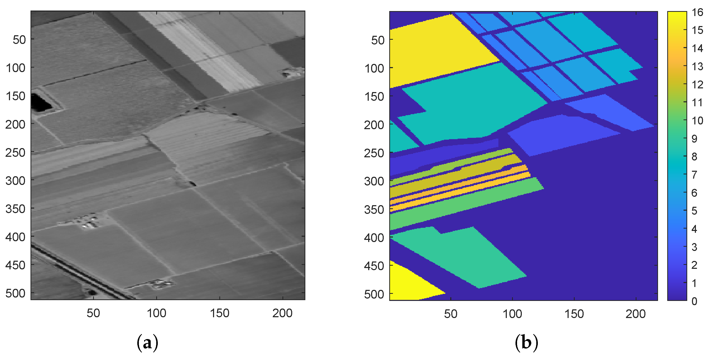
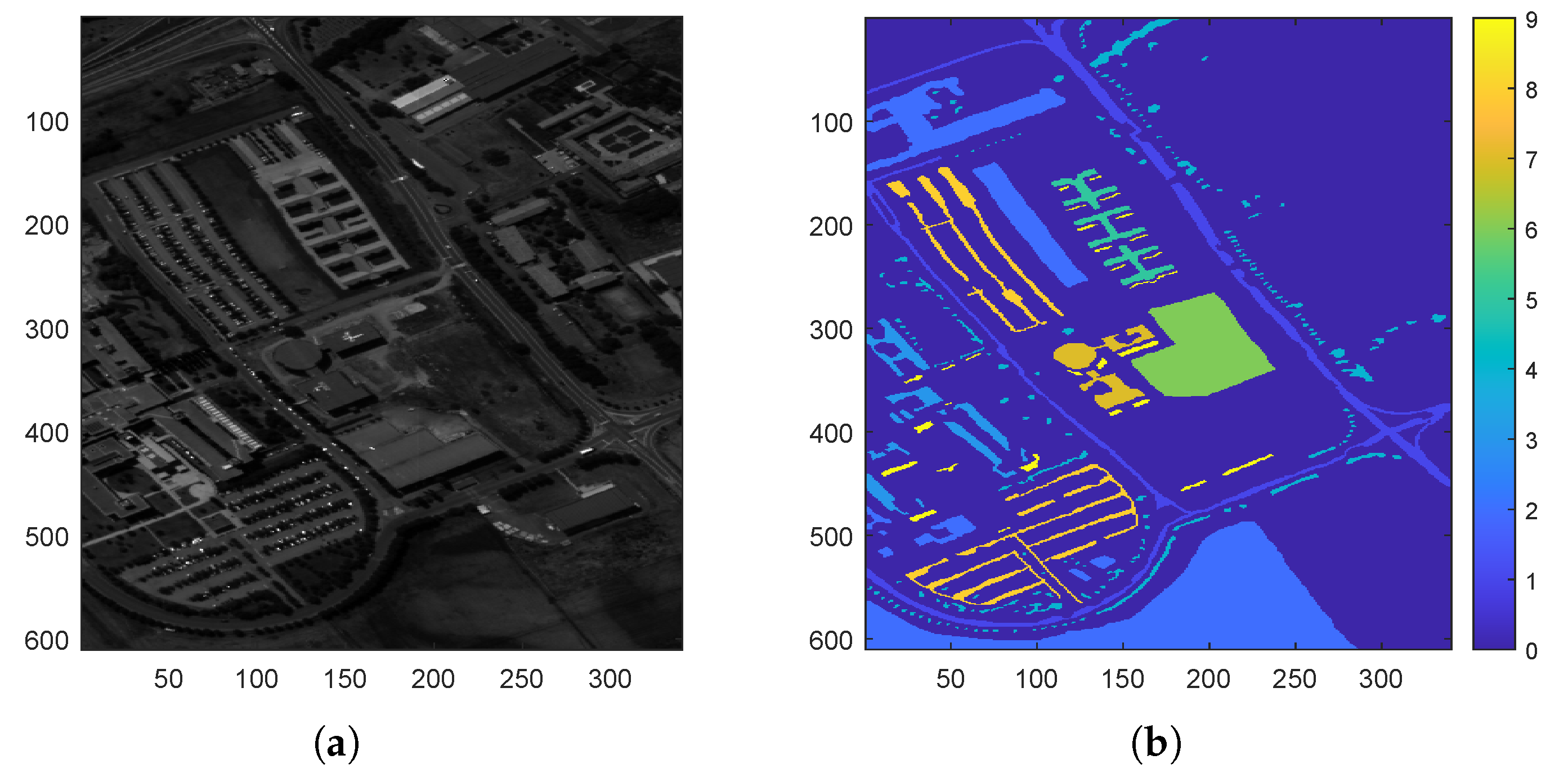
To assess the efficacy of ContrastBS, we compare ContrastBS with nine existing BS methods on three HSIs. The nine comparison methods include deep learning-based methods (i.e., BS network using convolutional neural networks (BS-Net-Conv) [20] and dual attention reconstruction network for BS (DARecNet-BS) [22]), machine learning-based method (i.e., manifold ranking (MR) [18]), point-wise method (i.e., OPBS [14]), and ranking-based methods without using deep learning algorithms (i.e., MVPCA [17], ECA [16], LCMV band correlation minimization (LCMVBCM) [15], LCMV band correlation constraint (LCMVBCC) [15], and SR-SSIM [8]). We briefly introduce the BS methods used for comparison as follows.

(1) BS-Net-Conv [20] is a generative algorithm-based method. This method leverages the autoencoder to mine band representativeness and selects the desired number of bands with high representation. Since the BS-Net-Conv method can take advantage of deep learning to model the nonlinear interdependences between bands, this method can achieve good classification performance.

(2) DARecNet-BS [22] is a deep learning-based BS method implemented with the help of the generative algorithm. DARecNet-BS uses a dual attention mechanism to recalibrate the feature maps and then uses the reconstruction network to restore the original HSIs, followed by selecting the bands with the highest entropy in the reconstructed output.

(3) MR [18] relies on advanced machine learning techniques, encompassing clustering, manifold learning, and clone selection, to perform its BS tasks.

(4) OPBS [14] selects, one by one, the bands that maximize the volume of the hypersphere formed by selected bands until the size of the selected band subset reaches the desired size.

(5) MVPCA [17] is frequently employed as a benchmark for the evaluation of BS methodologies due to its effectiveness and simplicity. MVPCA selects the bands with high discrimination ability, and the discrimination power of a band is gauged by the ratio of the variance of this band to the sum of variances across all bands.

(6) ECA [16] ranks the band priorities by assuming that exemplars are far from high-density points and have the largest local density.

(7) LCMVBCM [15] and LCMVBCC [15] select the desired bands by ranking the representative ability of each band to the entire image cube. BCC and BCM are used as specific evaluation criteria for LCMV, and the corresponding BS techniques are termed LCMVBCC and LCMVBCM, respectively.

(8) SR-SSIM [8] is a state-of-the-art similarity ranking-based BS method that uses the structural similarity metric to gauge the similarity between bands.

4.1.2. Datasets

The three HSIs used in the experiments are Indian Pines (IP), Salinas (SA), and Pavia University (PU).

(1) The IP dataset comprises 16 distinct land cover categories and 220 bands, each containing 145 × 145 pixels. Our experiments remove the water vapor absorption and low signal-to-noise ratio bands, including 1–3, 103–112, 148–165, and 217–220. The remaining 185 bands are used. The image in grayscale of band 170 and ground truth on the IP dataset are given in Figure 2.

Figure 2. IP dataset. (a) Image in grayscale of band 170. (b) Ground truth.

(2) The SA dataset consists of 224 bands, 16 different kinds of land cover, and 512 × 217 pixels. The image in grayscale of band 100 and ground truth on the SA dataset are given in Figure 3.

Figure 3. SA dataset. (a) Image in grayscale of band 100. (b) Ground truth.

(3) The PU dataset includes nine classes of land cover and 610 × 340 pixels. Moreover, 103 bands are contained in the PU dataset. Figure 4 presents the image in grayscale of band 50 and ground truth on the PU dataset.

Figure 4. PU dataset. (a) Image in grayscale of band 50. (b) Ground truth.

Table 1 presents the details of three hyperspectral datasets.

Table 1. Information on three hyperspectral datasets.

Dataset	Pixel	Band	Class
Indian Pines	145 × 145	185	16
Salinas	512 × 217	224	16
Pavia University	610 × 340	103	9

4.1.3. Classifier and Classification Evaluation Metrics

The support vector machine (SVM) classifier is utilized to evaluate the classification effectiveness of band subsets selected by different BS approaches. This classifier employs the Gaussian radial basis function [36] as its kernel function. The parameters of SVM are determined through cross-validation and grid search. Additionally, the one-against-all scheme is utilized for multi-class classification.

Furthermore, we make use of three evaluation metrics, i.e., overall accuracy (OA), average accuracy (AA), and kappa coefficient (Kappa), to quantitatively evaluate classification performance [20]. The error matrix of the classification results is denoted by $\mathbf{K}\in {\mathbb{R}}^{m\times m}$, where the value of position $(i,j)$ in $\mathbf{K}$ denotes the count of ith class samples classified as the jth class, and m represents the number of classes of land cover. Mathematically, AA, OA, and Kappa can be expressed as

$$\mathrm{AA}=\mathrm{mean}\left(\mathrm{diag}\right(\mathbf{K})./\mathrm{sum}(\mathbf{K},2\left)\right),$$

(11)

$$\mathrm{OA}=\mathrm{sum}\left(\mathrm{diag}\right(\mathbf{K}\left)\right)/\mathrm{sum}\left(\mathbf{K}\right),$$

(12)

$$\mathrm{Kappa}=\frac{\mathrm{OA}-\left(\mathrm{sum}(\mathbf{K},1)\mathrm{sum}(\mathbf{K},2)\right)/\mathrm{sum}{\left(\mathbf{K}\right)}^2}{1-\left(\mathrm{sum}(\mathbf{K},1)\mathrm{sum}(\mathbf{K},2)\right)/\mathrm{sum}{\left(\mathbf{K}\right)}^2},$$

(13)

where $\mathrm{mean}(·)$ stands for computing the mean over all samples, $\mathrm{diag}\left(\mathbf{K}\right)$ represents the vector of diagonal elements of $\mathbf{K}$, $./$ denotes the elementwise division operation, $\mathrm{sum}(·,2)$ represents summing over the elements of each row, $\mathrm{sum}(·)$ represents computing the sum of all elements, and $\mathrm{sum}(·,1)$ denotes summing over the elements of each column. The higher values of AA, OA, and Kappa indicate better performance in classification.

We randomly choose 10% of the samples from each category as the training set in each independent experiment, while the remaining samples are utilized for testing [37,38]. Table 2, Table 3 and Table 4 list the counts of training samples and testing samples for each category on three datasets. We use the average of accuracies obtained from five independent classification experiments as the final result.

Table 2. Number of training samples ($n_{\mathrm{train}}$) and number of testing samples ($n_{\mathrm{test}}$) for each category within IP.

Class	${\mathit{n}}_{\mathbf{train}}$	${\mathit{n}}_{\mathbf{test}}$
1. Alfalfa	5	49
2. Corn-notill	143	1291
3. Corn-mintill	83	751
4. Corn	23	221
5. Grass/pasture	49	448
6. Grass/trees	74	673
7. Grass/pasture-mowed	2	24
8. Hay-windrowed	48	441
9. Oats	2	18
10. Soybeans-notill	96	872
11. Soybeans-mintill	246	2222
12. Soybeans-clean	61	553
13. Wheat	21	191
14. Woods	129	1165
15. Buildings-grass-trees-drives	38	342
16. Stone-steel towers	9	86

Table 3. Number of training samples ($n_{\mathrm{train}}$) and number of testing samples ($n_{\mathrm{test}}$) for each land cover type within PU.

Class	${\mathit{n}}_{\mathbf{train}}$	${\mathit{n}}_{\mathbf{test}}$
1. Asphalt	663	5968
2. Meadows	1000	17,649
3. Gravel	209	1890
4. Trees	306	2758
5. Painted metal sheets	134	1211
6. Bare soil	502	4527
7. Bitumen	133	1197
8. Self-blocking bricks	368	3314
9. Shadows	94	853

Table 4. Number of training samples ($n_{\mathrm{train}}$) and number of testing samples ($n_{\mathrm{test}}$) for each category within SA.

Class	${\mathit{n}}_{\mathbf{train}}$	${\mathit{n}}_{\mathbf{test}}$
1. Weeds_1	200	1809
2. Weeds_2	372	3354
3. Fallow	197	1779
4. Fallow_rough_plow	139	1255
5. Fallow_smooth	267	2411
6. Stubble	395	3564
7. Celery	357	3222
8. Grapes_untrained	1000	10,271
9. Soil_vinyard_develop	620	5583
10. Corn_senesced_green_weeds	327	2951
11. Lettuce_romaine_4wk	106	962
12. Lettuce_romaine_5wk	192	1735
13. Lettuce_romaine_6wk	91	825
14. Lettuce_romaine_7wk	107	963
15. Vinyard_untrained	726	6542
16. Vinyard_vertical_trellis	180	1627

4.1.4. Hyper-Parameter Settings

The proposed ContrastBS uses the following hyper-parameter settings in this article. The momentum and weight decay of the SGD solver are $9\times {10}^{-1}$ and $1\times {10}^{-4}$, respectively. The size of a in the HSI patch ${\mathbf{X}}_{\mathrm{p}}\in {\mathbb{R}}^{a\times a\times B}$ is 10. The step size s of the window movement is set to one. The initial learning rate is equal to $6.25\times {10}^{-3}$, and a cosine decay schedule is employed to regulate the learning rate. The random Gaussian blur in the data augmentation strategy is configured to be applied with a probability of $20\%$, using a randomly selected $3\times 3$ Gaussian kernel with a standard deviation ranging from 1 to 2. The kernel size of the 1D convolutional layer in the band attention module is three. The batch size is 32. The penalty parameter $\eta$ is set to $1\times {10}^{-2}$.

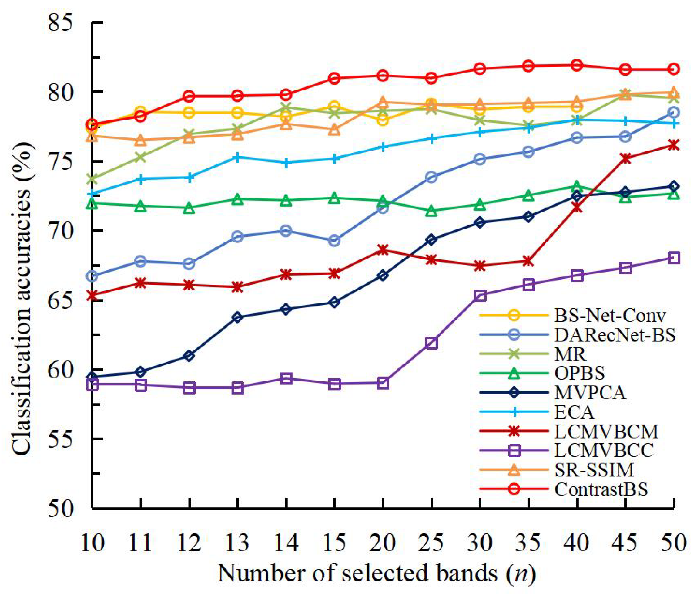
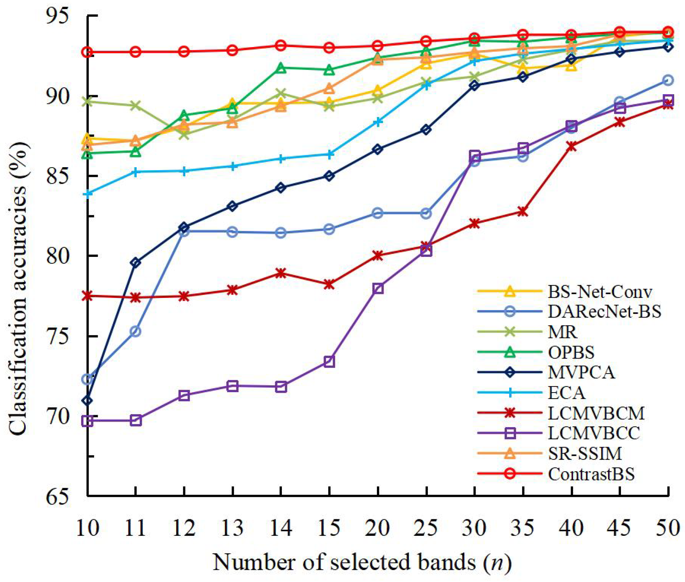
4.2. Classification Performance Comparison with Other BS Methods

To validate the usefulness of ContrastBS, we conduct a comparative assessment of its classification performance against nine existing BS methods across three hyperspectral datasets. Figure 5, Figure 6 and Figure 7 depict the OA curves of different BS methods employing the SVM classifier on three datasets. Table 5, Table 6 and Table 7 summarize the OAs, AAs, and Kappa values obtained by ContrastBS and the compared BS methods based on the SVM classifier on three datasets. In Table 5, Table 6 and Table 7, the best results are denoted by bold formatting.

Figure 5. Overall accuracy curves of different BS techniques on the IP dataset.

Figure 6. Overall accuracy curves of different BS techniques on the PU dataset.

Figure 7. Overall accuracy curves of different BS techniques on the SA dataset.

Table 5. Classification performance of BS techniques on the IP dataset.

	OA (%)	AA (%)	Kappa
1. BS-Net-Conv	78.91	72.27	0.7591
2. DARecNet-BS	69.25	61.90	0.6467
3. MR	78.42	71.24	0.7391
4. OPBS	72.33	62.97	0.6832
5. MVPCA	64.81	50.83	0.5960
6. ECA	75.16	65.25	0.7159
7. LCMVBCM	66.90	60.98	0.6186
8. LCMVBCC	58.95	49.74	0.5241
9. SR-SSIM	74.06	65.73	0.7396
10. ContrastBS	80.94	74.01	0.7821

Table 6. Classification performance of BS techniques on the PU dataset.

	OA (%)	AA (%)	Kappa
1. BS-Net-Conv	87.31	77.11	0.8306
2. DARecNet-BS	72.28	62.01	0.6248
3. MR	89.61	79.03	0.8442
4. OPBS	86.39	76.28	0.8182
5. MVPCA	70.95	55.99	0.6129
6. ECA	83.86	71.88	0.7841
7. LCMVBCM	77.50	67.97	0.6896
8. LCMVBCC	69.70	63.76	0.5803
9. SR-SSIM	86.90	77.60	0.8244
10. ContrastBS	92.70	82.01	0.9025

Table 7. Classification performance of BS techniques on the SA dataset.

	OA(%)	AA (%)	Kappa
1. BS-Net-Conv	90.27	89.07	0.8916
2. DARecNet-BS	90.95	89.99	0.8990
3. MR	89.94	88.84	0.8970
4. OPBS	92.04	90.10	0.9111
5. MVPCA	84.91	84.10	0.8316
6. ECA	92.01	90.23	0.9109
7. LCMVBCM	89.62	89.21	0.8659
8. LCMVBCC	87.88	87.82	0.8554
9. SR-SSIM	92.55	90.60	0.9169
10. ContrastBS	93.00	90.80	0.9220

4.2.1. IP Dataset

Figure 5 provides the OA curves of different BS techniques on the IP dataset when 10 to 50 bands are selected. As illustrated in Figure 5, the classification accuracy of ContrastBS significantly exceeds that of the competitors when more than twelve bands are used on the IP dataset. For example, ContrastBS can achieve relatively high classification accuracy when selecting twelve bands, while the other BS methods cannot obtain this accuracy even when the count of selected bands is expanded to fifty.

Table 5 summarizes the OAs, AAs, and Kappa values obtained by ContrastBS and other BS techniques when the count of selected bands is fifteen on the IP dataset. As presented in Table 5, ContrastBS yields the highest classification accuracy on the IP dataset. Furthermore, compared to the most competitive comparison technique (i.e., BS-Net-Conv), ContrastBS achieves a 2.03% and 1.74% increase in OA and AA, respectively. This experimental result demonstrates that the contrastive learning-based ContrastBS method, which can better utilize the abstract semantic information of the HSI, is able to select a more valuable subset of bands compared to the generative-based BS-Net-Conv method.

4.2.2. PU Dataset

Figure 6 presents the OA curves of the BS methods used for comparison and the proposed ContrastBS on PU. As given in Figure 6, our ContrastBS always surpasses the nine comparison methods in terms of classification performance when selecting different numbers of bands. Notably, ContrastBS requires only ten bands to achieve very high accuracy, while the advanced SR-SSIM and OPBS need more than thirty bands to obtain such accuracy. This experimental result demonstrates that ContrastBS can provide excellent classification accuracy even when the size of the selected band subset is limited.

Table 6 summarizes the OAs, AAs, and Kappa values obtained by ContrastBS and nine comparison methods when the count of selected bands is ten on PU. As summarized in Table 6, ContrastBS demonstrates a notable enhancement in terms of Kappa when compared to competitors. Additionally, ContrastBS is able to improve the OA by at least 3.09% and the AA by at least 2.98% compared to the comparison methods on the PU dataset, indicating that the proposed BS method can focus on the most valuable band subset with the help of the contrastive learning and the attention mechanism.

4.2.3. SA Dataset

Figure 7 draws the OA curves of the BS methods used for comparison and the proposed ContrastBS on SA. As displayed in Figure 7, our ContrastBS consistently achieves the highest OA under different sizes of band subsets on the SA dataset. It is worth noting that ContrastBS outperforms the generative algorithm-based BS methods (i.e., BS-Net-Conv and DARecNet-BS), which demonstrates the importance of considering the abstract semantic information of HSIs in the BS task. Furthermore, ContrastBS has obvious superiority over the comparison methods when using twenty bands. In addition, as shown in Figure 7, MR shows a decrease in classification accuracy with the increase in the number of selected bands when selecting more than twelve bands on the SA dataset, and this phenomenon can be interpreted in terms of the Hughes phenomenon.

Table 7 presents the OAs, AAs, and Kappa values obtained by ContrastBS and nine comparison methods when the count of selected bands is fifteen on SA. As presented in Table 7, for the SA dataset, although the best competitor (i.e., SR-SSIM) can obtain relatively high OA, AA, and Kappa, ContrastBS still attains the best classification performance due to its ability to well consider the abstract semantic information of the HSI and the nonlinear relationship between bands.

4.3. Analysis of Computational Time

Table 8 summarizes the computational times required for ContrastBS and nine comparison methods when selecting fifteen bands on the IP dataset. As summarized in Table 8, the deep learning-based BS methods (i.e., BS-Net-Conv, DARecNet-BS, and ContrastBS) require some time for network training. However, once the network is trained, BS-Net-Conv or ContrastBS exhibits a remarkably efficient inference time of just 0.0004 s, which is much less than the running times required for the BS methods without deep learning (i.e., MVPCA, LCMVBCC, LCMVBCM, ECA, OPBS, MR, and SR-SSIM). Since DARecNet-BS computes entropy for each band during inference, it requires a longer inference time than that required by BS-Net-Conv and ContrastBS.

Table 8. Comparison of computational times of BS techniques.

	MR	OPBS	MVPCA	ECA	LCMVBCM	LCMVBCC	SR-SSIM	BS-Net-Conv	DARecNet-BS	ContrastBS
Training Time (s)	4.79	0.74	0.13	1.97	1.64	3.18	35.91	18,050.45	3211.74	110.91
Inference Time (s)								0.0004	0.0137	0.0004

Furthermore, as listed in Table 8, when comparing the three deep learning-based BS methods, our ContrastBS costs much less time on network training than BS-Net-Conv and DARecNet-BS, which rely on generative algorithms. This experimental result demonstrates that the time cost required by our method is much lower than that required by generative algorithm-based BS methods, since the proposed contrastive learning-based BS method avoids the computationally expensive pixel-level reconstruction step commonly used in generative methods.

4.4. Analysis of Data Augmentation Strategies

To verify that the improved augmentation strategy can serve the HSI BS task more effectively than the traditional augmentation strategy originally designed for normal images, we compare the classification results of band subsets selected by the ContrastBS framework when using the traditional augmentation (i.e., including color distortion) and the improved augmentation (i.e., no color distortion), respectively, in Figure 8. The size of the selected band subset on each dataset in Figure 8 is consistent with that in Table 5, Table 6 and Table 7.

Figure 8. SVM classification maps of band subsets selected by the ContrastBS framework using the traditional data augmentation or the improved data augmentation. (a) Indian Pines—ground truth, (b) Indian Pines—traditional augmentation (OA = 78.62%, AA = 71.60%), (c) Indian Pines—improved augmentation (OA = 80.94%, AA = 74.01%), (d) Pavia University—ground truth, (e) Pavia University–traditional augmentation (OA = 88.60%, AA = 78.65%), (f) Pavia University—improved augmentation (OA = 92.70%, AA = 82.01%), (g) Salinas—ground truth, (h) Salinas—traditional augmentation (OA = 91.35%, AA = 90.14%), (i) Salinas—improved augmentation (OA = 93.00%, AA = 90.80%).

As shown in Figure 8, ContrastBS with improved augmentation strategy achieves better classification performance compared to ContrastBS with traditional augmentation strategy. For example, using the improved augmentation strategy helps ContrastBS achieve a 4.10% improvement in OA on the PU dataset compared to using the traditional augmentation strategy. The experimental results verify that the improved augmentation strategy can help the contrastive learning algorithm better serve the HSI BS task.

4.5. Ablation Study of the Loss Function

To verify the effectiveness of the designed loss function, we perform ablation studies on the symmetric loss constraint (i.e., Equation (7)) and sparsity constraint (i.e., Equation (8)) of the loss function, respectively. Table 9 lists the classification results achieved by the contrastive learning-based BS framework for selecting fifteen bands on the IP dataset when either a single constraint or two constraints (i.e., ContrastBS) are used for the loss function.

Table 9. Ablation studies on the symmetric loss constraint and sparsity constraint of the loss function.

Symmetric	Sparsity	OA (%)	AA (%)	Kappa
✔		67.17	60.30	0.6215
	✔	53.83	39.46	0.4569
✔	✔	80.94	74.01	0.7821

As shown in Table 9, the classification performance achieved by the band subset selected when the loss function uses both symmetric loss constraint and sparsity constraint is better than the classification performance achieved by the band subset selected when the loss function only uses a single constraint. Experimental results verify that the designed loss function containing symmetric loss constraint and sparsity constraint can help the contrastive learning-based BS framework select the most valuable band subset.

5. Discussion

According to the experiments in Section 4, we summarize some important results and discuss some interesting phenomena.

(1) Superiority and robustness of ContrastBS. From the experiments in Section 4.2, it is observed that our ContrastBS offers better overall classification performance on the three datasets compared to the competitors, demonstrating that the BS method implemented by means of the contrastive learning and attention mechanism is capable of selecting the most valuable band subset. It is worth noting that BS-Net-Conv, which is based on the generative algorithm, is able to achieve better classification performance on the IP dataset compared to the other comparison BS methods, while it performs worse than SR-SSIM and OPBS on the PU and SA datasets, as presented in Figure 5, Figure 6 and Figure 7. By contrast, the proposed ContrastBS attains better performance than the comparison methods on all three datasets, indicating that ContrastBS is robust to the datasets. The experimental results verify that the contrastive learning-based BS method has a stronger generalization ability compared to the generative-based BS method.

(2) Computational efficiency of ContrastBS. In terms of computational efficiency, the experiments in Section 4.2 and Section 4.3 demonstrate that ContrastBS is able to select the required band subset within a reasonable time. Furthermore, ContrastBS implemented with the help of contrastive learning can avoid the computationally costly generation step in generative-based BS methods, resulting in a more efficient unsupervised representation learning-based BS process. The results of comparing the training time of ContrastBS with that of BS-Net-Conv and that of DARecNet-BS in Table 8 confirm the above statement.

6. Conclusions

In this paper, we propose a contrastive learning-based unsupervised BS architecture, termed ContrastBS, which can mine the abstract semantic information of HSIs. In ContrastBS, we introduce the attention mechanism into the contrastive learning framework to extract the importance of each band. Moreover, we improve the traditional data augmentation strategy originally designed for normal images in SimSiam to make contrastive learning better serve HSIs. In addition, we design a loss function, which can constrain the symmetric loss while ensuring attention to the most valuable bands, specifically for the contrastive learning-based BS network. Experimental results indicate that the implemented ContrastBS has excellent performance compared to the comparison BS methods. In the future, we will explore other effective unsupervised representation learning techniques for the HSI BS task, aiming to enhance efficiency and effectiveness.

References

- Sun, X.; Shen, X.; Pang, H.; Fu, X. Multiple Band Prioritization Criteria-Based Band Selection for Hyperspectral Imagery. Remote Sens. 2022, 14, 5679. [Google Scholar] [CrossRef]
- Liu, K.H.; Chen, Y.K.; Chen, T.Y. A Band Subset Selection Approach Based on Sparse Self-Representation and Band Grouping for Hyperspectral Image Classification. Remote Sens. 2022, 14, 5686. [Google Scholar] [CrossRef]
- Wang, X.; Qian, L.; Hong, M.; Liu, Y. Dual Homogeneous Patches-Based Band Selection Methodology for Hyperspectral Classification. Remote Sens. 2023, 15, 3841. [Google Scholar] [CrossRef]
- Song, M.; Shang, X.; Wang, Y.; Yu, C.; Chang, C.I. Class Information-Based Band Selection for Hyperspectral Image Classification. IEEE Trans. Geosci. Remote Sens. 2019, 57, 8394–8416. [Google Scholar] [CrossRef]
- Sun, W.; Yang, G.; Peng, J.; Meng, X.; He, K.; Li, W.; Li, H.C.; Du, Q. A Multiscale Spectral Features Graph Fusion Method for Hyperspectral Band Selection. IEEE Trans. Geosci. Remote Sens. 2022, 60, 1–12. [Google Scholar] [CrossRef]
- Chang, C.I.; Kuo, Y.M.; Chen, S.; Liang, C.C.; Ma, K.Y.; Hu, P.F. Self-Mutual Information-Based Band Selection for Hyperspectral Image Classification. IEEE Trans. Geosci. Remote Sens. 2021, 59, 5979–5997. [Google Scholar] [CrossRef]
- Liu, Y.; Li, X.; Xu, Z.; Hua, Z. BSFormer: Transformer-Based Reconstruction Network for Hyperspectral Band Selection. IEEE Geosci. Remote Sens. Lett. 2023, 20, 1–5. [Google Scholar] [CrossRef]
- Xu, B.; Li, X.; Hou, W.; Wang, Y.; Wei, Y. A Similarity-Based Ranking Method for Hyperspectral Band Selection. IEEE Trans. Geosci. Remote Sens. 2021, 59, 9585–9599. [Google Scholar] [CrossRef]
- Li, X.; Zhang, W.; Niu, S.; Cao, Z.; Zhao, L. Kernel-OPBS Algorithm: A Nonlinear Feature Selection Method for Hyperspectral Imagery. IEEE Geosci. Remote Sens. Lett. 2020, 17, 464–468. [Google Scholar] [CrossRef]
- Liu, Y.; Li, X.; Hua, Z.; Xia, C.; Zhao, L. A Band Selection Method with Masked Convolutional Autoencoder for Hyperspectral Image. IEEE Geosci. Remote Sens. Lett. 2022, 19, 1–5. [Google Scholar] [CrossRef]
- Zhang, W.; Li, X.; Zhao, L. Discovering the Representative Subset with Low Redundancy for Hyperspectral Feature Selection. Remote Sens. 2019, 11, 1341. [Google Scholar] [CrossRef]
- Singh, P.S.; Karthikeyan, S. Enhanced classification of remotely sensed hyperspectral images through efficient band selection using autoencoders and genetic algorithm. Neural Comput. Appl. 2022, 34, 21539–21550. [Google Scholar] [CrossRef]
- Liu, Y.; Li, X.; Feng, Y.; Zhao, L.; Zhang, W. Representativeness and Redundancy-Based Band Selection for Hyperspectral Image Classification. Int. J. Remote Sens. 2021, 42, 3534–3562. [Google Scholar] [CrossRef]
- Zhang, W.; Li, X.; Dou, Y.; Zhao, L. A geometry-based band selection approach for hyperspectral image analysis. IEEE Trans. Geosci. Remote Sens. 2018, 56, 4318–4333. [Google Scholar] [CrossRef]
- Chang, C.I.; Wang, S. Constrained band selection for hyperspectral imagery. IEEE Trans. Geosci. Remote Sens. 2006, 44, 1575–1585. [Google Scholar] [CrossRef]
- Sun, K.; Geng, X.; Ji, L. Exemplar component analysis: A fast band selection method for hyperspectral imagery. IEEE Geosci. Remote Sens. Lett. 2015, 12, 998–1002. [Google Scholar]
- Chang, C.I.; Du, Q.; Sun, T.L.; Althouse, M.L. A joint band prioritization and band-decorrelation approach to band selection for hyperspectral image classification. IEEE Trans. Geosci. Remote Sens. 1999, 37, 2631–2641. [Google Scholar] [CrossRef]
- Wang, Q.; Lin, J.; Yuan, Y. Salient band selection for hyperspectral image classification via manifold ranking. IEEE Trans. Neural Netw. Learn. Syst. 2016, 27, 1279–1289. [Google Scholar] [CrossRef]
- Sun, W.; Peng, J.; Yang, G.; Du, Q. Fast and Latent Low-Rank Subspace Clustering for Hyperspectral Band Selection. IEEE Trans. Geosci. Remote Sens. 2020, 58, 3906–3915. [Google Scholar] [CrossRef]
- Cai, Y.; Liu, X.; Cai, Z. BS-Nets: An End-to-End Framework for Band Selection of Hyperspectral Image. IEEE Trans. Geosci. Remote Sens. 2020, 58, 1969–1984. [Google Scholar] [CrossRef]
- Zhang, H.; Sun, X.; Zhu, Y.; Xu, F.; Fu, X. A Global-Local Spectral Weight Network Based on Attention for Hyperspectral Band Selection. IEEE Geosci. Remote Sens. Lett. 2022, 19, 1–5. [Google Scholar] [CrossRef]
- Roy, S.K.; Das, S.; Song, T.; Chanda, B. DARecNet-BS: Unsupervised Dual-Attention Reconstruction Network for Hyperspectral Band Selection. IEEE Geosci. Remote Sens. Lett. 2021, 18, 2152–2156. [Google Scholar] [CrossRef]
- Chen, T.; Kornblith, S.; Norouzi, M.; Hinton, G. A simple framework for contrastive learning of visual representations. In Proceedings of the International Conference on Machine Learning, Vienna, Austria, 13–18 July 2020; pp. 1597–1607. [Google Scholar]
- Grill, J.B.; Strub, F.; Altché, F.; Tallec, C.; Richemond, P.; Buchatskaya, E.; Doersch, C.; Avila Pires, B.; Guo, Z.; Gheshlaghi Azar, M.; et al. Bootstrap your own latent-a new approach to self-supervised learning. Adv. Neural Inf. Process. Syst. 2020, 33, 21271–21284. [Google Scholar]
- Chen, X.; He, K. Exploring simple siamese representation learning. In Proceedings of the IEEE/CVF Conference on Computer Vision and Pattern Recognition, Nashville, TN, USA, 20–25 June 2021; pp. 15750–15758. [Google Scholar]
- Hadsell, R.; Chopra, S.; LeCun, Y. Dimensionality reduction by learning an invariant mapping. In Proceedings of the 2006 IEEE Computer Society Conference on Computer Vision and Pattern Recognition (CVPR’06), New York, NY, USA, 17–22 June 2006; IEEE: Piscataway, NJ, USA, 2006; Volume 2, pp. 1735–1742. [Google Scholar]
- Wu, Z.; Xiong, Y.; Yu, S.X.; Lin, D. Unsupervised feature learning via non-parametric instance discrimination. In Proceedings of the IEEE Conference on Computer Vision and Pattern Recognition, Salt Lake City, UT, USA, 18–23 June 2018; pp. 3733–3742. [Google Scholar]
- He, K.; Fan, H.; Wu, Y.; Xie, S.; Girshick, R. Momentum contrast for unsupervised visual representation learning. In Proceedings of the IEEE/CVF Conference on Computer Vision and Pattern Recognition, Seattle, WA, USA, 13–19 June 2020; pp. 9729–9738. [Google Scholar]
- Bahdanau, D.; Cho, K.; Bengio, Y. Neural Machine Translation by Jointly Learning to Align and Translate. In Proceedings of the 3rd International Conference on Learning Representations, San Diego, CA, USA, 7–9 May 2015. [Google Scholar]
- Galassi, A.; Lippi, M.; Torroni, P. Attention in natural language processing. IEEE Trans. Neural Netw. Learn. Syst. 2020, 32, 4291–4308. [Google Scholar] [CrossRef]
- Subakan, C.; Ravanelli, M.; Cornell, S.; Bronzi, M.; Zhong, J. Attention Is All You Need In Speech Separation. In Proceedings of the ICASSP 2021—2021 IEEE International Conference on Acoustics, Speech and Signal Processing (ICASSP), Toronto, ON, Canada, 6–11 June 2021; pp. 21–25. [Google Scholar] [CrossRef]
- Sun, H.; Zheng, X.; Lu, X.; Wu, S. Spectral–Spatial Attention Network for Hyperspectral Image Classification. IEEE Trans. Geosci. Remote Sens. 2020, 58, 3232–3245. [Google Scholar] [CrossRef]
- Li, X.; Ding, J. Spectral–Temporal Transformer for Hyperspectral Image Change Detection. Remote Sens. 2023, 15, 3561. [Google Scholar] [CrossRef]
- Dou, Z.; Gao, K.; Zhang, X.; Wang, H.; Han, L. Band selection of hyperspectral images using attention-based autoencoders. IEEE Geosci. Remote Sens. Lett. 2020, 18, 147–151. [Google Scholar] [CrossRef]
- Guo, M.H.; Xu, T.X.; Liu, J.J.; Liu, Z.N.; Jiang, P.T.; Mu, T.J.; Zhang, S.H.; Martin, R.R.; Cheng, M.M.; Hu, S.M. Attention mechanisms in computer vision: A survey. Comput. Vis. Media 2022, 8, 331–368. [Google Scholar] [CrossRef]
- Tarabalka, Y.; Chanussot, J.; Benediktsson, J.A. Segmentation and classification of hyperspectral images using watershed transformation. Pattern Recognit. 2010, 43, 2367–2379. [Google Scholar] [CrossRef]
- Zhang, W.; Li, X.; Zhao, L. A Fast Hyperspectral Feature Selection Method Based on Band Correlation Analysis. IEEE Geosci. Remote Sens. Lett. 2018, 15, 1750–1754. [Google Scholar] [CrossRef]
- Sui, C.; Li, C.; Feng, J.; Mei, X. Unsupervised Manifold-Preserving and Weakly Redundant Band Selection Method for Hyperspectral Imagery. IEEE Trans. Geosci. Remote Sens. 2020, 58, 1156–1170. [Google Scholar] [CrossRef]
Disclaimer/Publisher’s Note: The statements, opinions and data contained in all publications are solely those of the individual author(s) and contributor(s) and not of MDPI and/or the editor(s). MDPI and/or the editor(s) disclaim responsibility for any injury to people or property resulting from any ideas, methods, instructions or products referred to in the content. |
© 2023 by the authors. Licensee MDPI, Basel, Switzerland. This article is an open access article distributed under the terms and conditions of the Creative Commons Attribution (CC BY) license (https://creativecommons.org/licenses/by/4.0/).