Article

Evaluating the Transferability of Spectral Variables and Prediction Models for Mapping Forest Aboveground Biomass Using Transfer Learning Methods

1
Research Center of Forestry Remote Sensing & Information Engineering, Central South University of Forestry and Technology, Changsha 410004, China
2
Key Laboratory of Forestry Remote Sensing Based Big Data & Ecological Security for Hunan Province, Changsha 410004, China
3
Key Laboratory of State Forestry Administration on Forest Resources Management and Monitoring in Southern Area, Changsha 410004, China
*
Author to whom correspondence should be addressed.
Remote Sens. 2023, 15(22), 5358; https://doi.org/10.3390/rs15225358
Submission received: 28 September 2023 / Revised: 30 October 2023 / Accepted: 6 November 2023 / Published: 14 November 2023
(This article belongs to the Section Biogeosciences Remote Sensing)

Abstract

:
Forests, commonly viewed as the Earth’s lungs, play a crucial role in mitigating greenhouse gas emissions, regulating the globe, and maintaining ecological equilibrium. The assessment of aboveground biomass (AGB) serves as a pivotal indicator for evaluating forest quality. By integrating remote sensing images with a small number of ground-measured samples to map, forest AGBs can significantly reduce time and labor costs. Current research mainly focuses on improving the accuracy of mapping forest AGBs, such as integrating multiple-sensors remote sensing data and models. However, due to uncertainties associated with remote sensing images and complexities inherent in forest structures, the accuracy of mapping forest AGBs is constrained by both the quantity and distribution of ground samples available. The development of transfer learning methods can fully utilize ground-based measurement data and enable the application of samples across regions and time. To evaluate the potential of transfer learning methods in mapping forest AGBs, this study conducted a spatial–temporal transfer of spectral variables (SVs) and prediction models (PMs) using a direct-push transfer method, and a new evaluation metric, relative change of R-squared (RCRS), was proposed to assess the transferability of SVs and PMs. The results showed that the transferability of SVs and PMs in the spatial target domain is obviously greater than that in the temporal target domain. Compared to the temporal target domain, the RCRS for transfer SVs in the spatial target domain was lower by 20.89 (oak) and 20.88 (Chinese fir) and for transfer PMs by 24.16 (oak) and 24.79 (Chinese fir). Tree species is also one of the main factors affecting the spatial and temporal transfer of SVs, and it is challenging to transfer SVs between different tree species. The results also show that nonparametric models have better generalization performance, and their transferability is much greater than that of parametric models.

1. Introduction

Regarded as the largest organic carbon reservoir, forests play an indispensable role in promoting the global carbon cycle and buffering global warming [1,2,3]. Forest aboveground biomass (AGB) is viewed as one of the most important indicators for assessing the carbon sequestration capacity [4,5,6,7]. Therefore, it is meaningful to accurately and efficiently map the forest AGB and obtain the spatial distribution information for guiding rational forest management activities [8,9,10]. Thanks to the timeliness and economy of remote sensing data, the combination of remote sensing images with a small amount of ground-measured data has great potential to replace traditional ground-measured work [11,12,13]. Furthermore, in comparison with SAR and LiDAR data, optical remote sensing data have been widely applied to map the forest AGB in large regions because of the short return period, the mature image processing technology, and the rich spatial and spectral resolutions [14,15,16].
Because of their timeliness and cheapness, previous studies have proved that combining optical remote sensing data with a small amount of ground-measured samples are an effective means to map forest AGBs at large scales [9,14,16]. The accuracy of mapping forest AGB is highly related to the number and quality of employed ground samples [17,18]. Furthermore, mapping forest AGB in different regions and different years also requires corresponding ground samples that match the acquisition time of the remote sensing images. However, it is rather difficult to obtain so many ground-measured samples for dynamic monitoring at large scales [5,7,8,9,19,20].
Recently, transfer learning methods have been successfully applied to remote sensing image classification and target recognition [21,22,23,24,25,26]. Their main idea is to extract and train transferable remote sensing variables and a priori models from existing labelled samples and then apply them to another target domain to be identified [23,25,27,28,29]. For mapping forest AGB, the performance of traditional machine learning algorithms depends on the number of training and test samples and whether they are independently distributed [27,28,30]. In contrast, transfer learning methods do not necessitate a specific distribution of training and test samples, enabling the reuse of samples [23,24,25,26,27]. Transfer learning methods can give full play to the values of ground-measured samples and realize the transfer application in temporal and cross-region remote sensing images [31,32,33,34]. Therefore, to reduce the dependence on the ground samples, it is valuable to evaluate the potential of transfer learning methods for mapping forest AGB in the homogeneous forest using the same type of remote sensing images.
Additionally, the application of transfer learning methods in mapping forest aboveground biomass (AGB) typically relies on assessing the transferability of variables derived from remote sensing imagery and prediction models. Moreover, feature selection and modelling are two indispensable parts to apply the transfer learning methods for mapping forest AGB. Previous studies have been devoted to how to improve the accuracy of mapping forest AGB, such as developing a wide variety of feature selection algorithms and integrating learning models [35,36,37]. However, most of the research focuses on methods to improve accuracy, ignoring the generalization performance and transferability of variables and prediction models. Although some studies have yielded promising results, the stability and generalization performance of models have been questioned. Therefore, it is necessary to further explore the spatial and temporal transferability of spectral variables (SVs) and predictive models (PMs) using transfer learning methods and remote sensing images for mapping forest AGB.
Moreover, the spectral information of forests in complex ecosystems is often influenced by multiple environmental factors, such as tree species, soil conditions, topographic features, temperature, and precipitation [38,39,40,41,42]. These limitations in interpreting the relationships between spectral variables and forest AGB hinder the establishment of stable models between spectral variables and forest AGB, thereby affecting the generalization performance and transferability of remotely sensed variables and prediction models used for mapping forest AGB. Additionally, studies have demonstrated significant variations in generalization performance among models; parametric models tend to exhibit inferior generalization performance compared to nonparametric models, while integrated learning algorithms generally outperform single models [8,14,36]. Therefore, it is necessary to further explore the transferability of spectral variables and prediction models.
The objective of this study is to evaluate the transferability of SVs and PMs for mapping forest aboveground biomass (AGB) using remote sensing images with limited ground-measured samples. In this study, remotely sensed images and ground samples collected in different years and regions were divided into three domains: the source domain, the temporal target domain, and the spatial target domain. Firstly, we employed the distance correlation coefficient to rank and filter the variables in the source domain dataset. Subsequently, four models including random forest (RF), support vector machine (SVM), K-nearest neighbor (KNN), and multiple linear regression (MLR) were constructed to map forest AGB across the entire study area. Then, we applied a direct-push transfer learning approach to transfer the optimal set of SVs and models to both temporal and spatial target domains, respectively. Finally, we calculated the relative change in R-square as an evaluation metric to evaluate the transferability of spectral variables and prediction models in fir and oak forests.

2. Study Area and Data

2.1. Study Area

The study area is in and around Xiangtan City, Hunan Province, China, with geographical coordinates ranging from 111°58′ to 113°05′E and from 27°20′55″ to 28°05′40″N. It encompasses a total area of over 10,000 km2. This region falls within the subtropical humid climate zone, characterized by an average annual temperature ranging from 16.7 to 17.4 °C and an average annual precipitation ranging from 1200 mm to 1500 mm. The elevation of the study area ranges from 30 m to 800 m above sea level, predominantly consisting of low mountains and hills. Geomorphologically, the study area exhibits higher elevations in its northern, western, and southern parts while displaying flatter terrain in the central and eastern regions; however, there is minimal variation in relief across the landscape. Approximately 80% of the land lies below an altitude of 150 m above sea level. As of 2022, the forest coverage exceeds 45%. The primary tree species found here include Chinese fir, oak, and others.

2.2. Ground Data

The field survey data for this study were collected in 2009, 2014, and 2019, encompassing two tree species: Chinese fir and oak. All sample plots were distributed across three areas in Xiangtan City (XT), Ningxiang City (NX), and Wangcheng District (WC) (Figure 1). Each plot was designed as a square measuring 25 × 25 m, with the GPS coordinates of its four corner points recorded. For each tree with a diameter at breast height (DBH) greater than 5 cm within each sample plot, both DBH and height measurements were taken. The volume of each tree was calculated using the binary product equation, which was then input into the biomass conversion equation to obtain individual tree biomass values. The binary volume equations for single wood samples are shown in Equations (1) (Chinese fir) and (2) (oak).
V = 0.000050479055 × D 1.9085054 × H 0.99076507
V = 0.00005877042 × D 1.9699831 × H 0.89646157
where V is the volume of individual wood samples, D is the diameter at breast height, and H is the height of the tree. The biomass conversion equation for fir and oak is shown in Equation (3).
B = a × V + b
where B is biomass, a is 0.3999 (fir) or 1.1453 (oak), and b is 22.541 (fir) or 8.5473 (oak). Summing up the biomass of all trees within each plot yielded the plot-level biomass. Table 1 lists the statistical information of ground samples in the three areas.

2.3. Remote Sensing Data and Pre-Processing

The remote sensing data (Table 2) used in this study include Landsat 5 TM and Landsat 8 OLI from the online datasets provided by GEE (https://developers.google.com/earthengine/datasets/, accessed on 2 November 2013). Of these, Landsat 5 TM was taken in 2009 and Landsat 8 OLI was taken in 2014 and 2019, with each cloud-free image covering the study area composited from a time series of images within a year. To improve the quality of the acquired images, pre-processing of the images, including radiation correction, atmospheric correction, and terrain correction, is required. In addition, relative radiometric corrections are performed on images acquired at different times to keep the radiometric scales consistent from image to image. All these image processing operations are implemented in the GEE platform.

2.4. Extraction and Selection of SV

2.4.1. Extraction of SVs

SVs, such as spectral reflectance and vegetation indices extracted from remote sensing images, are widely utilized for land type monitoring and the assessment of vegetation health. Vegetation indices, obtained through algebraic combinations of spectral reflectance, enable dimensionless measurements of surface vegetation status. The selected vegetation indices for this study include the normalized difference vegetation index (NDVI), atmospherically resistant vegetation index (ARVI), red–green vegetation index (RGVI), enhanced vegetation index (EVI), soil-adjusted vegetation index (SAVI), difference vegetation index (DVI), and ratio vegetation index (RVI). These indices have demonstrated strong correlations with forest growth states and hold significant potential in estimating aboveground biomass.

2.4.2. Selection of Optimal Variables

The selection of an appropriate combination of variables can effectively enhance the performance and efficiency of prediction models [8,36]. Correlation coefficients are commonly employed to evaluate the sensitivity between SVs and forest AGBs [4,6,8]. While Pearson’s correlation coefficient is a widely used statistical metric for linear correlation assessment, it may not adequately capture the non-linear relationships between SVs and AGB in complex forest ecosystems [6]. To provide a comprehensive description of the relationships between SVs and AGBs, distance correlation coefficients (DC) were employed in this study to evaluate their correlation. Initially, the distance correlation coefficients between SVs and forest AGBs were computed, and sorted variables were obtained in descending order. Then, the forward feature selection method was applied to get the optimal feature set by stepwise addition of predictor variables until no further improvement in model accuracy was observed.

2.5. AGB Estimation Model and Spatial–Temporal Transfer

2.5.1. Machine Learning Models

Machine learning algorithms have gained widespread adoption in recent years for mapping forest aboveground biomass (AGB) due to their efficient and robust predictive performance. In this study, three machine learning models, namely, KNN, RF, and SVM, were employed to establish the relationships between SVs and forest AGBs. Additionally, the parametric regression method (MLR) was also employed for comparative analysis alongside machine learning models [4,6,8,13,14,15,36]. These models were implemented using packages integrated within R software 4.2.0.

2.5.2. Transfer Learning

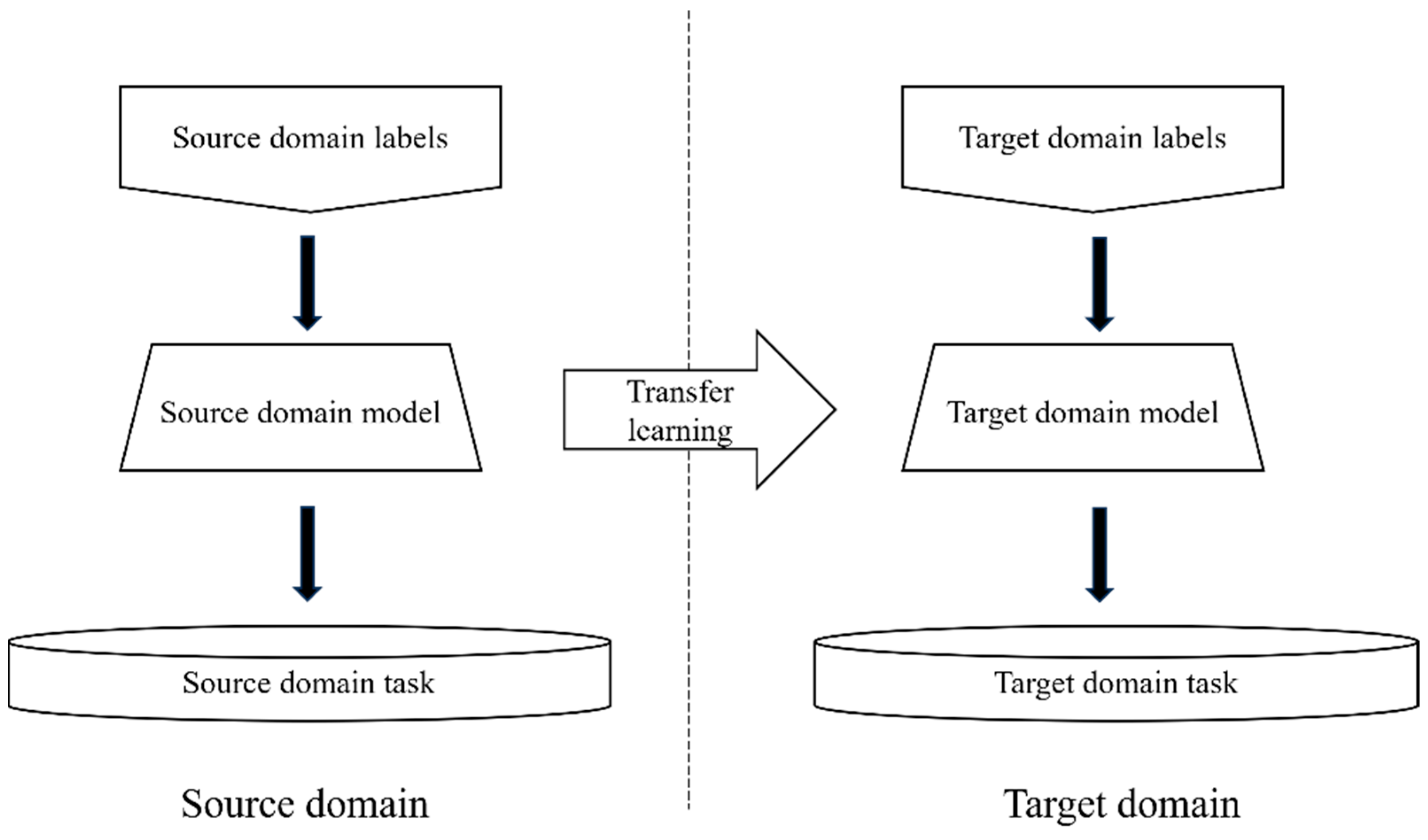
In conventional machine learning algorithms, the process of selecting features and training models for each task leads to repetitive tasks, which not only reduces efficiency but also limits model interpretability and generalization performance. In contrast, transfer learning methods have the potential to enhance model performance and improve data utilization efficiency in complex scenarios characterized by insufficient data, high task relevance, sensor differences, and sample imbalance [23,24,25]. The concept of transfer learning, as shown in Figure 2, optimizes the model training process in the target domain by transferring the model trained using the source domain data labels to the target domain.
By exploiting task similarities, transfer learning enables samples’ reuse and facilitates efficient training of models using remote sensing data. Therefore, transfer learning holds great promise for forest biomass remote sensing mapping applications as it can potentially enhance model performance, reduce data dependency, and optimize data utilization efficiency while addressing challenges such as diverse sensor datasets, geographic regions variations, and time series analysis.

2.5.3. Spatial–Temporal Transfer of Mapping Forest AGB

To assess the transferability of models at both temporal and spatial target domains, a transudative inference method was employed to transfer the SVs and PMs temporally and spatially. The samples of the Xiangtan area collected in 2014 were considered as the source domain, while the samples collected in 2009 and 2019 in the same area served as temporal target domains for evaluating the transferability of remote sensing features and prediction models over time. Additionally, keeping the source domain unchanged, samples from the NX and WC areas in 2014 were used as spatial target domains to test the transferability of features and prediction models at a spatial scale.
The application of transfer learning methods in mapping forest aboveground biomass (AGB) typically relies on assessing the transferability of variables derived from remote sensing imagery and prediction models. Figure 3 illustrates the spatial–temporal transfer process of mapping forest AGB, which consists of two parts: firstly, transferring selected spectral variables from the source to target domain followed by training a model using target domain samples; secondly, conducting feature selection and model training within the source domain before transferring both the features and the trained model to the target domains together. Furthermore, spectral variables and training models were also selected based on samples from target domains for comparison with the prediction results after the optimal feature set or model transfers.

2.6. Transfer Model Evaluation

For machine learning models, the widely adopted K-fold cross-validation technique was employed to train and optimize the model parameters, with K set to 10 in this study. To assess the performance of each model, we utilized the coefficient of determination, mean square error (RMSE), and relative root mean square error (rRMSE) as metrics for evaluating model accuracies. Lower values of RMSE and rRMSE, closer to zero, along with higher values of R2, closer to one, indicate more precise prediction results from the model. The calculation formulas are as follows:
R 2 = 1 ( y i y ^ i ) 2 ( y i y ^ i ) 2
R M S E = 1 N i = 1 N y i y ^ i 2
r R M S E = R M S E y ¯ × 100 %
where N is number of samples, y is the observed value of AGB, y ^ is the predicted value of AGB, and y ¯ is the average of the observed AGB for all samples.
Additionally, in the context of machine learning models, R-square serves as a metric for assessing the goodness of fit in regression models, indicating the extent to which the variation in the dependent variable can be elucidated by the independent variable. In transfer learning models, apart from commonly employed accuracy evaluation metrics, it is necessary to evaluate of the potential of transfer learning quantitatively. In this study, a novelty evaluation metric, named the relative change in R-square (RCRS), is proposed to assess the performance of transfer models in terms of data fitting. The formula of RCRS is as follows:
R C R S = R 2 ¯ R 2 R 2 ¯ × 100 %
where R 2 ¯ denotes the R-square of the model before transfer and R 2 denotes the R-square of the model after transfer. A smaller RCR implies a lesser decline in model fitting performance following spatial–temporal transfer, thereby indicating higher transferability. Conversely, a lower transferability is indicated by a larger decrease in model fitting performance.

3. Results

3.1. Analyzing Temporal and Spatial Variation of SVs

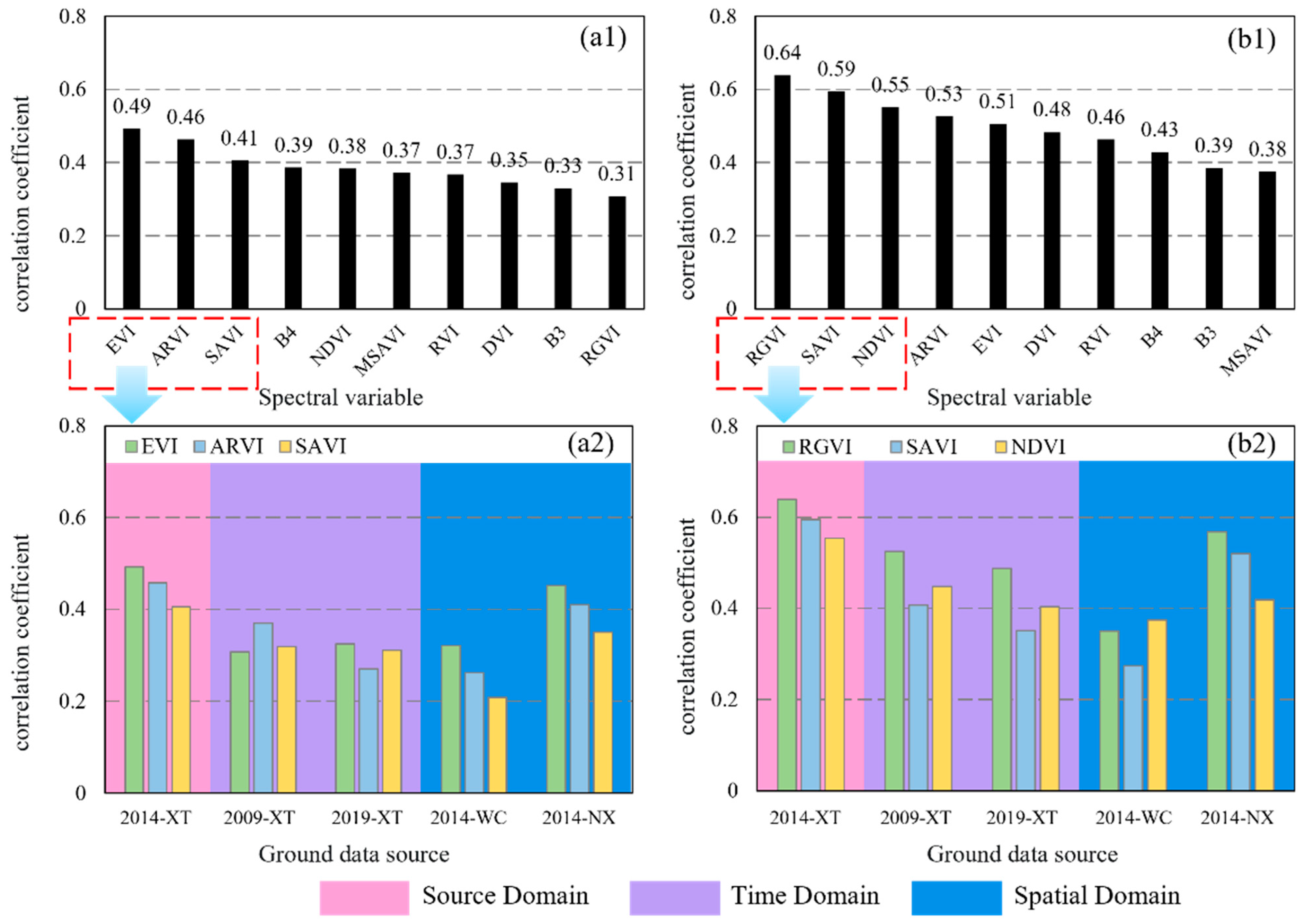
The distance correlation coefficients between the aboveground biomass (AGB) and the variables were calculated by aligning the ground survey data and remote sensing images with independent datasets from different times and regions, respectively. The top ten variables are shown in Figure 4(a1,b1), while the three most significant optical variables are highlighted by the red dashed lines in Figure 4. The sensitivity between SVs and forest AGB varies significantly across different tree species. Specifically, for oak sample plots, the distance correlation coefficients for all variables were ranged from 0.31 to 0.49, with EVI, ARVI, and SAVI being the top three SVs exhibiting respective distance correlation coefficients of 0.49, 0.46, and 0.41. For Chinese fir samples, the distance correlation coefficients for optical variables ranged from 0.38 to 0.64.
Moreover, the dominant spectral variables for Chinese fir forests were identified as EVI, ARVI, and SAVI, while RGVI, SAVI, and NDVI were found to be the prominent ones for oak forests in the source domain. Additionally, it was observed that the correlation coefficients between spectral variables and forest AGBs in oak forests were significantly higher compared to those in Chinese fir forests. It is also implied that the transfer ability of spectral features among tree species poses a considerable challenge.
To further investigate the temporal and spatial variability of features, we conducted an additional analysis on the dominant spectral variables in Chinese fir forests (EVI, ARVI, and SAVI) and oak forests (RGVI, SAVI, and NDVI). The DC coefficients between forest AGBs and these spectral features in different temporal and spatial domains are depicted in Figure 4(a2,b2). In the targeted temporal domain, substantial variations of DC coefficients were observed for the selected dominant spectral variables in both Chinese fir and oak forests. Specifically, the DC value of SAVI decreased from 0.59 (2014-XT) to 0.35 (2019-XT) in oak forests. These findings suggest that drastic changes in the temporal behavior of spectral variables can significantly impact the reliability of transfer learning models. Conversely, variations of DC coefficients associated with selected dominant spectral variables were considerably smaller in the spatial domain compared to those observed in the temporal domain. This implies that spectral variables possess a greater transferability within spatial domains than within temporal domains.

3.2. Mapping Forest AGB in Source Domains

In this study, each dataset was initially treated as an independent domain, and the optimal variable set was obtained from sorted alternative variables using the same variable selection methods, respectively. Moreover, the relationships between the forest aboveground biomass (AGB) and SVs of two tree species were established in each domain using four models: K-nearest neighbors (KNN), support vector regression (SVR), random forest (RF), and regression (MLR).
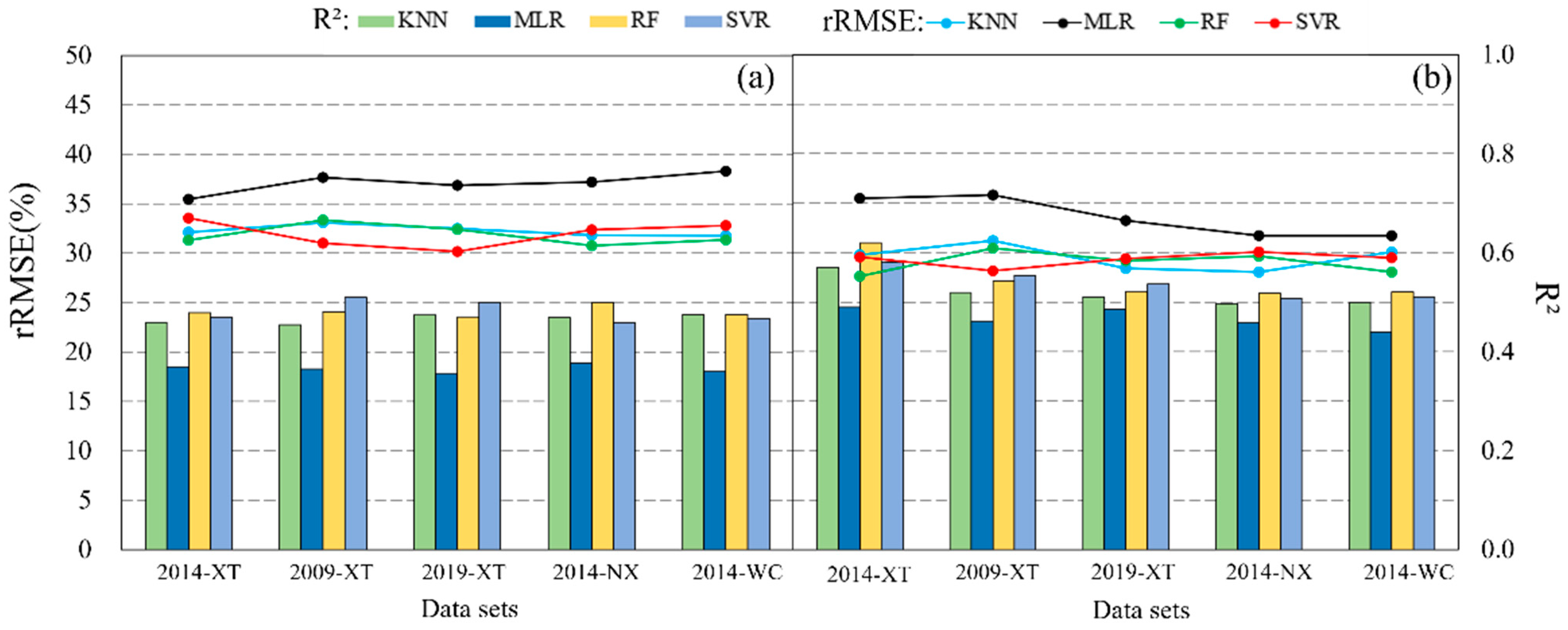
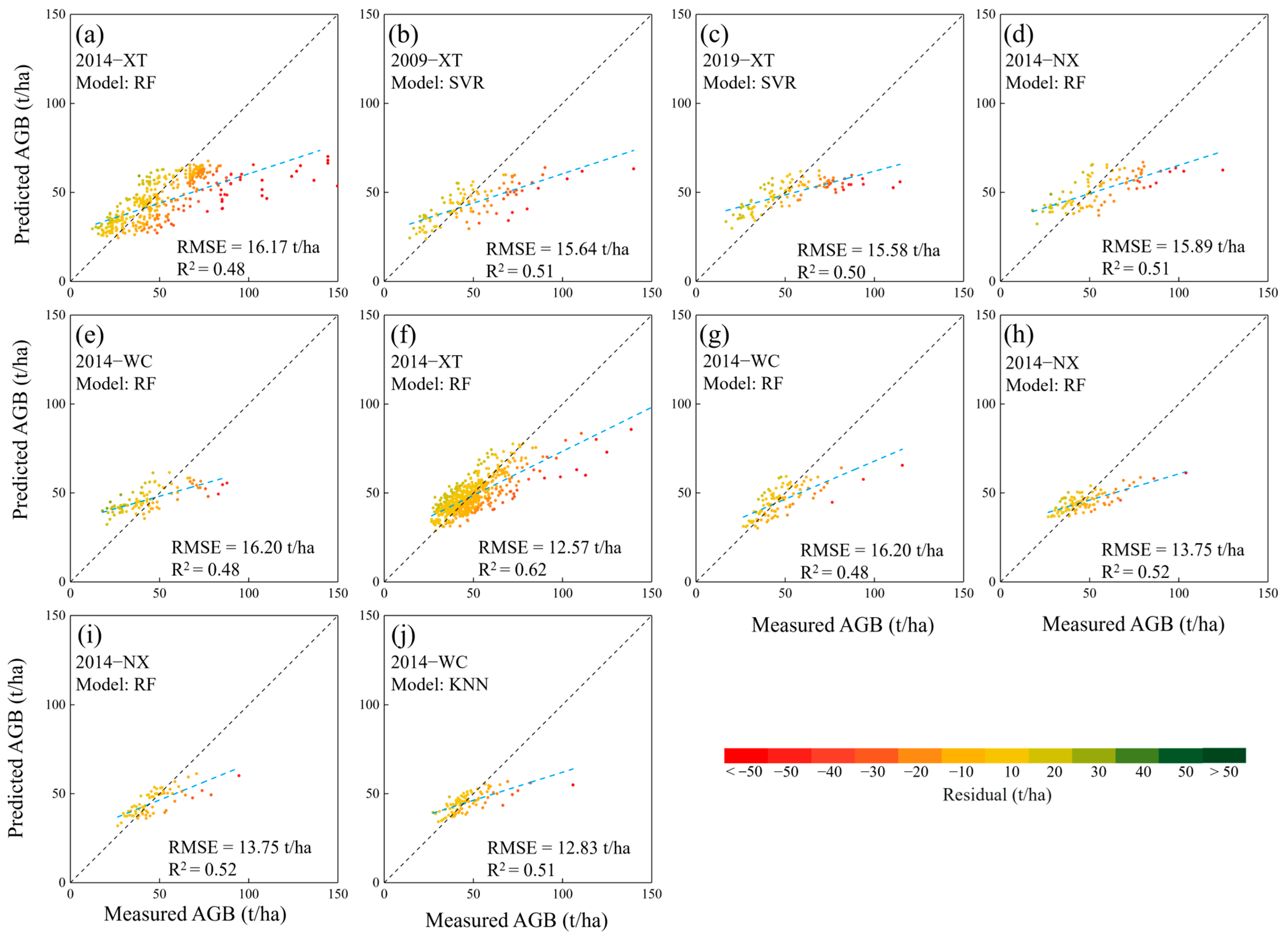
Figure 5 illustrates the coefficient of determination (R2) and relative root mean square (rRMSE) derived from the ground-measured and predicted forest AGB of the two tree species in each domain. It was observed that three machine learning algorithms exhibited a similar prediction performance, which significantly outperformed the MLR algorithm. Notably, the accuracy of mapping forest AGB in Chinese fir forests is slightly higher than that in oak forests across all models, with R2 ranging from 0.51 to 0.62 and RMSE ranging from 12.57 to 13.84 t/ha for Chinese fir forests, while R2 ranged from 0.48 to 0.51 and RMSE ranged from 15.58 to 16.20 t/ha for oak forests. The results showed that accuracies of mapping forest AGB can maintain a certain stability using remote sensing images and corresponding ground-measured samples in source domains.
To further analyze the results of mapping forest AGBs, the optimal model of each domain was selected, respectively. Scatterplots and residuals between the ground-measured and estimated forest AGBs are illustrated in Figure 6. Limits to the effect of the spectral saturation, overestimation, and underestimation of AGB for both tree species within each domain frequently occurred. Especially, the saturation levels were obviously less than 100 t/ha in both tree species.

3.3. Ttransferability of Spectral Variables in Mapping Forest AGB

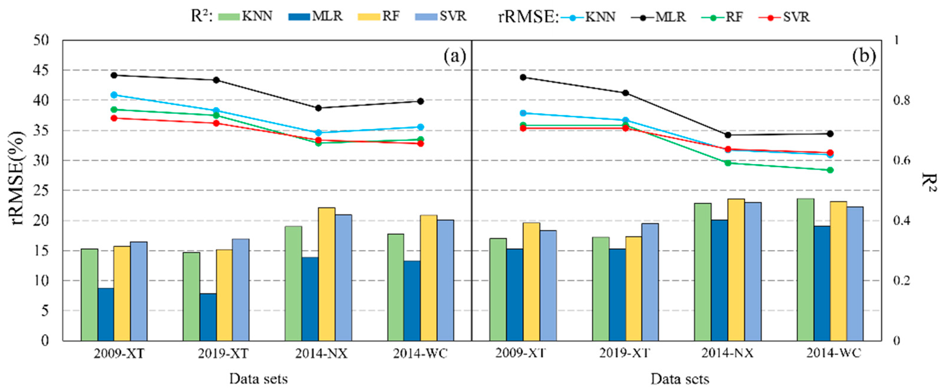
To investigate the transferability of SVs across different temporal and spatial domains, we transferred the optimal variable set obtained from the source domain dataset to both a temporal target domain (collected from samples in Xiangtan area in 2009 and 2019) and a spatial target domain (collected from samples in Ningxiang and Wangcheng areas in 2014). Subsequently, we retrained each model for four forest aboveground biomass (AGB) estimations to ensure their optimal performance. Four accuracy indicators, such as the determination coefficient, RMSE, rRMSE, and RCRS, were employed to evaluate the transferability of spectral variables.
The accuracy metrics for mapping AGB after the spatial–temporal transfer of spectral variables are presented in Figure 7. Transferring the same spectral variable set to both temporal and spatial domains resulted in a significant decrease in the accuracy of mapping forest AGB. Moreover, the accuracy of mapping forest AGB was notably lower in the temporal domain compared to the spatial domain, with the rRMSE ranging from 36.18% to 44.17% for oak and ranging from 35.37% to 43.83% for Chinese fir in the temporal domain, while ranging from 33.36% and 39.83% for oak and ranging from 28.47% to 34.44% for Chinese fir in the spatial domain. The results suggest that spectral variables demonstrate greater transferability in the spatial domain compared to that in the temporal domain. Furthermore, it is observed that machine learning models (KNN, SVM, and RF) exhibit higher transferability than parameter models (MLR) both in spatial and temporal domain transfers.
The scatter plots of optimal models in each domain were utilized to further analyze the transferability of spectral variables in both temporal and spatial domains (Figure 8). The results also indicated that the transferability of spectral variables was slightly higher in the spatial domain (R2: ranged from 0.43 to 0.49) compared to that in the temporal domain (R2: ranged from 0.34 to 0.39). Additionally, it was observed that tree species influenced the transferability of spectral variables, with oak forests exhibiting greater dispersion in the scatter plots when compared to Chinese fir forests. Specifically, R2 values ranged from 0.34 to 0.45 for oak forests and ranged from 0.39 to 0.47 for Chinese fir forests, respectively. Therefore, it can be inferred that spectral variables extracted from Chinese fir forests are more suitable for applying transfer learning than those extracted from oak forests.
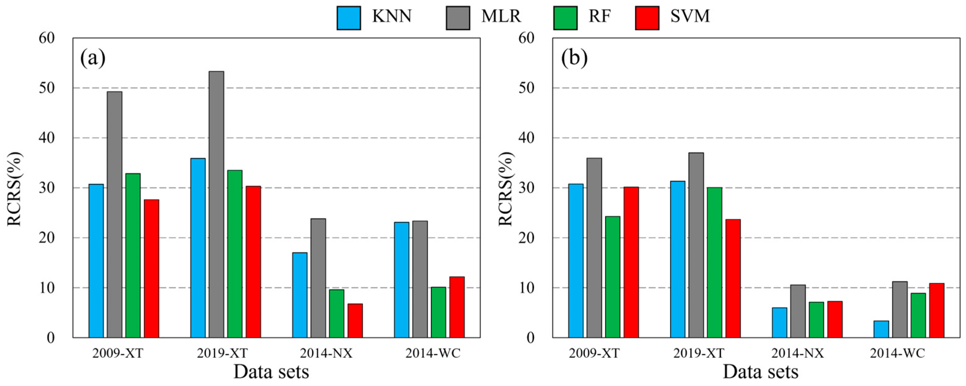
To further assess the transferability, the proposed metric was utilized to quantitatively describe the transfer performance of the models. In this study, RCRS values were computed based on the determination coefficients before and after applying transfer learning, and the corresponding histograms are presented in Figure 9. For both species, SVs transferred from the temporal domain exhibited significantly higher RCRS values compared to those transferred from the spatial domain. Moreover, for both tree species, the MLR model achieved a higher RCRS after spatial–temporal feature transfer than the machine learning model did; similarly, the oak forest AGB prediction model outperformed the Chinese fir forest AGB prediction model in terms of the RCRS. These findings suggested that tree species plays a crucial role in influencing SV nonparametric models demonstrating greater transferability as compared to parametric ones.

3.4. Transferability of Prediction Models in Mapping Forest AGB

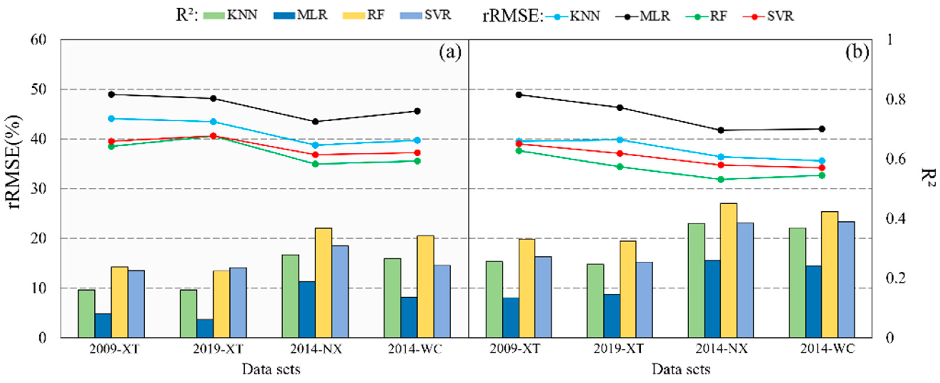
To evaluate the transferability of the prediction models, the trained models and optimal variables set derived from the source domain data were transferred to both spatial and temporal domains. In this study, all models were trained in the source domain and subsequently applied to temporal and spatial target domains. Then, the transferability of prediction models was evaluated by the performance of prediction models in mapping the forest AGB. Figure 10 illustrates the mapping accuracies (R2 and rRMSE) of forest AGB in the target domains with the trained models and optimal variables set derived from the source domain.
Compared with the results of the spectral variables transferring in the target domain, the mapping accuracy forest aboveground biomass (AGB) using transferred PMs is significantly reduced in both temporal and spatial domains, with relative root mean square errors (rRMSE) exceeding 35% for the oak forest and 30% for the Chinese fir forest. Similar to the transfer of spectral variables, the mapping accuracy of forest AGBs using transferred PMs was notably lower in the temporal domain compared to that in the spatial domain. Additionally, the AGB mapping accuracy in Chinese fir forests was higher than that in oak forests, with rRMSEs ranging from 38.55% to 48.97% for oak and ranging from 35.12% to 48.94% for Chinese fir in the temporal domains, while ranging from 35.56% to 39.76% for oak and ranging from 31.87% to 42.05 for Chinese fir in the spatial domains. The results indicate that predictive models are more transferable within spatial domains than within temporal domains, and nonparametric models exhibit greater transportability compared to parametric models. However, satisfactory mapping accuracy of forest AGB was not achieved in either temporal or spatial domains; thus, it remains challenging to simultaneously transfer spectral variables and predictive models across both temporal and spatial dimensions.
Scatter plots of the optimal model in each domain are employed to further analyze the transferability of PMs in the spatial–temporal domain (Figure 11). Compared with the results of spectral variables transferring in the target domain, the scatter plots of transferred PMs showed greater dispersion, with R2 ranging from 0.24 to 0.37 for oak and ranging from 0.33 to 0.44 for Chinese fir. Additionally, we observed a similar phenomenon as that observed for transferring spectral variables: the fit of the transfer model was superior in Chinese fir forests compared to oak forests, as well as being more effective in capturing spatial variations rather than temporal variations. These findings suggest that transferring both spectral variables and predictive models into the spatial–temporal domain poses significant challenges, particularly within oak forests.
To further analyze and quantify the transferability of PMs, Figure 12 illustrates the relative cross-region similarity (RCRS) when transferring each model trained in the source domain to both temporal and spatial domains. It is shown that the nonparametric model exhibits significantly lower RCRS compared to the parametric model, while PMs demonstrate notably lower RCRS in the spatial domain than in the temporal domain. These results indicate that the RF model displays superior transferability among all models examined. Moreover, PMs exhibit higher transferability within the spatial domain, particularly in Chinese fir forests rather than oak forests.

4. Discussion

4.1. Factors Affecting Transferability

Previous studies have demonstrated the strong correlation between forest aboveground biomass (AGB) and vegetation indices derived from optical imagery, indicating their potential for mapping forest AGB [3,4,5,6,7,8,13,14,15,36]. Similarly, our study also confirmed the feasibility of using optical remote sensing data for mapping forest AGB. However, limited transferability hinders the widespread adoption of remote sensing in AGB mapping with a small number of ground samples. Therefore, it is essential to analyze the transferability of SVs and PMs to promote and validate transfer learning methods. Our findings revealed that when transferred to different spatial–temporal target domains, SVs and PMs struggle to maintain their predictive accuracy due to the complex nature of forest ecosystems which leads to an unstable relationship between SVs and forest AGB. Li et al. also reported significant variations in optimal variable selection when changing remotely sensed data types or acquisition times [8,14].
In this study, we explored the transferability of SVs and PMs and found that transferability was significantly greater in the spatial domain than in the temporal domain. The spatial transferability is mainly reflected in the sharing of a similar topography, soil type, and vegetation composition among different geographical regions. The spatial target domains and spatial source domains of this study were both in Hunan Province, China, with similar geographic conditions (temperature, precipitation, elevation, etc.) associated with vegetation growth, similar forest stand conditions (soil type), and similar vegetation types so that the SVs and the PMs could be transferred from one spatial domain to another in a complete manner. In contrast, the variability of data in the temporal target and source domains mainly comes from the effects of climate change, seasonal variations, and anthropogenic activities, which lead to uncertainty in the relationships between forest AGB and SVs. As a result, variables and model transfer over temporal domains are often challenged by data distribution drift [43,44,45].
Additionally, there exists a significant disparity in the mobility between oak and Chinese fir species, with Chinese fir exhibiting greater transportability. Chinese fir possesses a simplified canopy structure characterized by dense branching and foliage that can be approximated as a geometric cone. Therefore, the forest’s canopy structure is accurately captured by SVs. Consequently, SVs establish a more stable relationships with aboveground biomass (AGB) in Chinese fir forests. Conversely, oak forests feature wider canopies with intricate branch patterns and complex structures, resulting in a stochastic relationship between SVs and oak forest AGB. It undoubtedly poses challenges when attempting to transfer SVs and PMs to temporal and spatial domains. It is worth mentioning that we only obtained representative samples of coniferous and broadleaf species (cedar and oak), which can be further supplemented with studies on a wider range of tree species in subsequent studies.
The estimation of forest parameters has extensively employed both parametric and nonparametric models, with numerous studies demonstrating that nonparametric models exhibit superior prediction accuracy for forest aboveground biomass (AGB) compared to that of parametric models [4,6,8]. This superiority can be attributed to the absence of fixed assumptions regarding the model’s form and parameters in nonparametric models. Their flexible structure allows them to adapt to different data distributions and sample characteristics [6,12]. Instead of relying on a specific data distribution, nonparametric models learn the structure of the model directly from the data. Our study also confirmed this finding. Additionally, we assessed the transferability of three machine learning algorithms (RF, SVM, and KNN) along with multiple linear regression (MLR). The results indicate that machine learning algorithms possess significantly higher transferability than MLR; particularly, RF exhibits the highest level of transferability. These findings inferred that the flexibility and adaptivity inherent in nonparametric models enable them to better accommodate diverse types of data and variations across different samples, ultimately enhancing their ability to generalize new data.

4.2. Potential Methods to Enhance Transferability and Generalizability

Previous studies have demonstrated that satisfactory accuracy can be achieved in estimating forest aboveground biomass (AGB) by constructing empirical models (parametric and nonparametric models) using spectral variables extracted from optical remote sensing data [4,8,13,14,15,36]. However, these studies have primarily focused on improving estimation accuracy while neglecting the generalization performance of the results. Consequently, researchers may become overly confident in their obtained results. The premise of promoting the use of remote sensing technology to map forest AGB is to improve the generalization and transfer performance of the method. Therefore, it is equally important to improve the generalization and transfer performance of the mapping method and the mapping accuracy.
Although previous studies have shown that vegetation indices such as the NDVI and RVI are closely related to the growth status of forests, it is challenging to use these variables to directly interpret forest AGB [6,9,12]. This also directly leads to the difficulty of using the same vegetation indices to map the forest AGB in different vegetation areas. Therefore, improving the interpretability between variables and forest AGB and selecting variables with strong interpretability to map forest AGB is an effective means to improve the generalizability and transferability of the mapping methodology. Li, Liu, et al., showed that the increase of the forest AGB was largely reflected in the height of the forest [13,15]. Therefore, incorporating forest height information into the prediction model (e.g., canopy height model, CHM) can improve the transferability and generalization performance of the model.
In addition, forest AGB is affected by many factors, including soil conditions (e.g., soil structure, organic matter, soil fertility, soil moisture), topographic factors (e.g., elevation, aspect), and human-induced activities (different forms of management, such as selective recording) [6,16,17]. Current AGB estimation models are mainly based on remotely sensed data and do not take into account ancillary data. Exploring key variables from different data sources (remotely sensed data and ancillary data) and developing suitable models that can effectively include different kinds of variables can effectively improve the generalization performance and transferability of forest AGB mapping results. However, different source data have different quality issues and spatial resolutions, and it is costly to use different data sources in forest AGB modelling. More research is needed to explore the effective incorporation of remote-sensing-derived products into process-based ecosystem models to better explain the spatial distribution and dynamics of forest AGB.

5. Conclusions

To assess the potential of transfer learning methods in the temporal and spatial domains, we developed a new metric, RCRS, for analyzing and evaluating the transportability of SVs and PMs in two target domains. Additionally, we investigated the influencing factors that affect the transferability of mapping forest AGB using remote sensing. The results indicated that the transferability of SVs and PMs is always greater in the spatial target domain than in the temporal target domain. Tree species is one of the main factors affecting the spatial–temporal transfer of SVs; it is challenging to realize the transfer of SVs across tree species, and the transferability of SVs and PMs is greater in Chinese fir samples than in oak. The results also show that nonparametric models have better generalization performance, and their transferability is much greater than that of parametric models. This study explored the application of transfer learning in remote sensing estimations of forest biomass and assessed the transferability of SVs and PMs, especially considering the impact of variability in the geographic context and temporal data on the generalization ability of the models. In future work, there is a need to explore interpretable variables for mapping forest AGBs and to further investigate ways to enhance the transportability of SVs and PMs.

Author Contributions

Conceptualization, L.C., J.L., Z.L. and H.L.; methodology, L.C. and J.L.; software, L.C., H.L. and T.Z.; validation, L.C. and J.L.; formal analysis, L.C., P.Y., T.Z. and J.L.; investigation, H.L., J.L. and P.Y.; resources, H.L. and J.L.; data processing, L.C., P.Y. and H.L.; original draft, L.C. and J.L.; review and revision, L.C., J.L., Z.L. and H.L.; final editing: L.C. and J.L.; visualization, L.C., J.L. and H.L.; supervision, H.L. and J.L.; project administration, H.L. and J.L.; funding acquisition, H.L. and J.L. All authors have read and agreed to the published version of the manuscript.

Funding

This research was funded by the National Natural Science Foundation of China (Project number: 32171784), the Excellent Youth Project of the Scientific Research Foundation of the Hunan Provincial Department of Education (Project number: 21B0246).

Data Availability Statement

The observed GSV data from the sample plots and the spatial distribution data of forest resources presented in this study are available on request from the corresponding author. Those data are not publicly available due to privacy and confidentiality.

Conflicts of Interest

The authors declare no conflict of interest.

References

  1. Seidl, R.; Spies, T.A.; Peterson, D.L.; Stephens, S.L.; Hicke, J.A. Searching for resilience: Addressing the impacts of changing disturbance regimes on forest ecosystem services. J. Appl. Ecol. 2016, 53, 120–129. [Google Scholar] [CrossRef] [PubMed]
  2. Schimel, D.S. Terrestrial ecosystems and the carbon cycle. Glob. Chang. Biol. 2006, 1, 77–91. [Google Scholar] [CrossRef]
  3. Le Toan, T.; Quegan, S.; Davidson, M.; Balzter, H.; Paillou, P.; Papathanassiou, K.; Plummer, S.; Rocca, F.; Saatchi, S.; Shugart, H.; et al. The BIOMASS mission: Mapping global forest biomass to better understand the terrestrial carbon cycle. Remote Sens. Environ. 2011, 115, 2850–2860. [Google Scholar] [CrossRef]
  4. Jiang, F.; Kutia, M.; Sarkissian, A.J.; Lin, H.; Long, J.; Sun, H.; Wang, G. Estimating the Growing Stem Volume of Coniferous Plantations Based on Random Forest Using an Optimized Variable Selection Method. Sensors 2020, 20, 7248. [Google Scholar] [CrossRef]
  5. Long, J.; Lin, H.; Wang, G.; Sun, H.; Yan, E. Estimating the Growing Stem Volume of the Planted Forest Using the General Linear Model and Time Series Quad-Polarimetric SAR Images. Sensors 2020, 20, 3957. [Google Scholar] [CrossRef]
  6. Jiang, F.; Kutia, M.; Ma, K.; Chen, S.; Long, J.; Sun, H. Estimating the aboveground biomass of coniferous forest in Northeast China using spectral variables, land surface temperature and soil moisture. Sci. Total Environ. 2021, 785, 147335. [Google Scholar] [CrossRef]
  7. Xu, X.; Lin, H.; Liu, Z.; Ye, Z.; Li, X.; Long, J. A Combined Strategy of Improved Variable Selection and Ensemble Algorithm to Map the Growing Stem Volume of Planted Coniferous Forest. Remote Sens. 2021, 13, 4631. [Google Scholar] [CrossRef]
  8. Li, X.; Liu, Z.; Lin, H.; Wang, G.; Sun, H.; Long, J.; Zhang, M. Estimating the Growing Stem Volume of Chinese Pine and Larch Plantations based on Fused Optical Data Using an Improved Variable Screening Method and Stacking Algorithm. Remote Sens. 2020, 12, 871. [Google Scholar] [CrossRef]
  9. Lu, D. The potential and challenge of remote sensing-based biomass estimation. Int. J. Remote Sens. 2006, 27, 1297–1328. [Google Scholar] [CrossRef]
  10. Zheng, S.; Cao, C.; Dang, Y.; Xiang, H.; Zhao, J.; Zhang, Y.; Wang, X.; Guo, H. Retrieval of forest growing stock volume by two different methods using Landsat TM images. Int. J. Remote Sens. 2014, 35, 29–43. [Google Scholar] [CrossRef]
  11. Yang, C.; Huang, H.; Wang, S. Estimation of tropical forest biomass using Landsat TM imagery and permanent plot data in Xishuangbanna, China. Int. J. Remote Sens. 2011, 32, 5741–5756. [Google Scholar] [CrossRef]
  12. Lu, D.; Chen, Q.; Wang, G.; Liu, L.; Li, G.; Moran, E. A survey of remote sensing-based aboveground biomass estimation methods in forest ecosystems. Int. J. Digit. Earth 2014, 9, 63–105. [Google Scholar] [CrossRef]
  13. Li, G.; Xie, Z.; Jiang, X.; Lu, D.; Chen, E. Integration of ZiYuan-3 Multispectral and Stereo Data for Modeling Aboveground Biomass of Larch Plantations in North China. Remote Sens. 2019, 11, 2328. [Google Scholar] [CrossRef]
  14. Li, X.; Lin, H.; Long, J.; Xu, X. Mapping the Growing Stem Volume of the Coniferous Plantations in North China Using Multispectral Data from Integrated GF-2 and Sentinel-2 Images and an Optimized Feature Variable Selection Method. Remote Sens. 2021, 13, 2740. [Google Scholar] [CrossRef]
  15. Liu, Z.; Ye, Z.; Xu, X.; Lin, H.; Zhang, T.; Long, J. Mapping Forest Stock Volume Based on Growth Characteristics of Crown Using Multi-Temporal Landsat 8 OLI and ZY-3 Stereo Images in Planted Eucalyptus Forest. Remote Sens. 2022, 14, 5082. [Google Scholar] [CrossRef]
  16. Zhu, X.; Liu, D. Improving forest aboveground biomass estimation using seasonal Landsat NDVI time-series. ISPRS J. Photogramm. Remote Sens. 2015, 102, 222–231. [Google Scholar] [CrossRef]
  17. Reiche, J.; Hamunyela, E.; Verbesselt, J.; Hoekman, D.; Herold, M. Improving near-real time deforestation monitoring in tropical dry forests by combining dense Sentinel-1 time series with Landsat and ALOS-2 PALSAR-2. Remote Sens. Environ. 2018, 204, 147–161. [Google Scholar] [CrossRef]
  18. Narine, L.L.; Popescu, S.C.; Malambo, L. Synergy of ICESat-2 and Landsat for Mapping Forest Aboveground Biomass with Deep Learning. Remote Sens. 2019, 11, 1503. [Google Scholar] [CrossRef]
  19. Chrysafis, I.; Mallinis, G.; Siachalou, S.; Patias, P. Assessing the relationships between growing stock volume and Sentinel-2 imagery in a Mediterranean forest ecosystem. Remote Sens. Lett. 2017, 8, 508–517. [Google Scholar] [CrossRef]
  20. Gasparri, N.I.; Parmuchi, M.G.; Bono, J.; Karszenbaum, H.; Montenegro, C.L. Assessing multi-temporal Landsat 7 ETM+ images for estimating above-ground biomass in subtropical dry forests of Argentina. J. Arid Environ. 2010, 74, 1262–1270. [Google Scholar] [CrossRef]
  21. Gu, Q.Z.J. Learning the Shared Subspace for Multi-task Clustering and Transductive Transfer Classification. In Proceedings of the International Conference on Data Mining (ICDM 2009), Miami Beach, FL, USA, 6–9 December 2009. [Google Scholar]
  22. Zhou, Y.; Lian, J.; Han, M. Remote Sensing Image Transfer Classification Based on Weighted Extreme Learning Machine. IEEE Geosci. Remote Sens. Lett. 2016, 13, 1405–1409. [Google Scholar] [CrossRef]
  23. Luo, Y.; Liu, T.; Tao, D.; Xu, C. Decomposition-Based Transfer Distance Metric Learning for Image Classification. IEEE Trans. Image Process. 2014, 23, 3789–3801. [Google Scholar] [CrossRef]
  24. George, D.; Shen, H.; Huerta, E.A. Classification and unsupervised clustering of LIGO data with Deep Transfer Learning. Phys. Rev. D 2018, 97, 101501. [Google Scholar] [CrossRef]
  25. Saba, L.; Agarwal, M.; Sanagala, S.; Gupta, S.; Sinha, G.; Johri, A.; Khanna, N.; Mavrogeni, S.; Laird, J.; Pareek, G.; et al. Brain MRI-based Wilson disease tissue classification: An optimised deep transfer learning approach. Electron. Lett. 2020, 56, 1395–1398. [Google Scholar] [CrossRef]
  26. Imoto, K.; Nakai, T.; Ike, T.; Haruki, K.; Sato, Y. A CNN-Based Transfer Learning Method for Defect Classification in Semiconductor Manufacturing. IEEE Trans. Semicond. Manuf. 2019, 32, 455–459. [Google Scholar] [CrossRef]
  27. Zhao, K.; Popescu, S.; Meng, X.; Pang, Y.; Agca, M. Characterizing forest canopy structure with lidar composite metrics and machine learning. Remote Sens. Environ. 2011, 115, 1978–1996. [Google Scholar] [CrossRef]
  28. Yao, J.; Raffuse, S.M.; Brauer, M.; Williamson, G.J.; Bowman, D.M.; Johnston, F.H.; Henderson, S.B. Predicting the minimum height of forest fire smoke within the atmosphere using machine learning and data from the CALIPSO satellite. Remote Sens. Environ. 2018, 206, 98–106. [Google Scholar] [CrossRef]
  29. Pan, S.J.; Yang, Q. A Survey on Transfer Learning. IEEE Trans. Knowl. Data Eng. 2010, 22, 1345–1359. [Google Scholar] [CrossRef]
  30. Ma, Y.; Luo, G.; Zeng, X.; Chen, A. Transfer learning based cross-company software defects prediction. Comput. Eng. Des. 2012, 54, 248–256. [Google Scholar] [CrossRef]
  31. Celestin, B.N.; Yunfei, S. The impact of learner characteristics on training transfer expectation: A survey of Thai teachers’ perception of cloud computing tools. Int. J. Train. Dev. 2018, 22, 256–273. [Google Scholar] [CrossRef]
  32. De Bruijne, M. Machine learning approaches in medical image analysis: From detection to diagnosis. Med. Image Anal. 2016, 33, 94–97. [Google Scholar] [CrossRef] [PubMed]
  33. Van Opbroek, A.; Achterberg, H.C.; Vernooij, M.W.; De Bruijne, M. Transfer Learning for Image Segmentation by Combining Image Weighting and Kernel Learning. IEEE Trans. Med. Imaging 2018, 38, 213–224. [Google Scholar] [CrossRef] [PubMed]
  34. Zhou, Y.; Wong, L.N.Y.; Tse, K.K.C. Retraction Note: Novel Rock Image Classification: The Proposal and Implementation of RockNet. Rock Mech. Rock Eng. 2023, 56, 3859. [Google Scholar] [CrossRef]
  35. Dube, T.; Sibanda, M.; Shoko, C.; Mutanga, O. Stand-volume estimation from multi-source data for coppiced and high forest Eucalyptus spp. silvicultural systems in KwaZulu-Natal, South Africa. ISPRS J. Photogramm. Remote Sens. 2017, 132, 162–169. [Google Scholar] [CrossRef]
  36. Jiang, F.; Zhao, F.; Ma, K.; Li, D.; Sun, H. Mapping the Forest Canopy Height in Northern China by Synergizing ICESat-2 with Sentinel-2 Using a Stacking Algorithm. Remote Sens. 2021, 13, 1535. [Google Scholar] [CrossRef]
  37. Wang, Y.; Zhang, X.; Guo, Z. Estimation of tree height and aboveground biomass of coniferous forests in North China using stereo ZY-3, multispectral Sentinel-2, and DEM data. Ecol. Indic. 2021, 126, 107645. [Google Scholar] [CrossRef]
  38. Wu, J.; Wang, T.; Pan, K.; Li, W.; Huang, X. Assessment of forest damage caused by an ice storm using multi-temporal remote-sensing images: A case study from Guangdong Province. Int. J. Remote Sens. 2016, 37, 3125–3142. [Google Scholar] [CrossRef]
  39. Jucker, T.; Caspersen, J.; Chave, J.; Antin, C.; Barbier, N.; Bongers, F.; Dalponte, M.; van Ewijk, K.Y.; Forrester, D.I.; Haeni, M.; et al. Allometric equations for integrating remote sensing imagery into forest monitoring programmes. Glob. Chang. Biol. 2016, 23, 177–190. [Google Scholar] [CrossRef]
  40. Mauro, F.; Molina, I.; García-Abril, A.; Valbuena, R.; Ayuga-Téllez, E. Remote sensing estimates and measures of uncertainty for forest variables at different aggregation levels. Environmetrics 2016, 27, 225–238. [Google Scholar] [CrossRef]
  41. Gibson, R.K.; Collins, L. A remote sensing approach to mapping fire severity in south-eastern Australia using sentinel 2 and random forest. Remote Sens. Environ. 2020, 240, 111702. [Google Scholar] [CrossRef]
  42. Miller, Z.M.; Hupy, J.; Chandrasekaran, A.; Shao, G.; Fei, S. Application of Postprocessing Kinematic Methods with UAS Remote Sensing in Forest Ecosystems. J. For. 2021, 119, 454–466. [Google Scholar] [CrossRef]
  43. Elhenawy, M.; Rakotonirainy, A.; Young, K.; Haworth, N.; Grazbieta, R.; Williamson, A. Detecting Driver Distraction in the ANDS Data using Pre-trained Models and Transfer Learning. In Proceedings of the Australasian Road Safety Conference, Adelaide, SA, Australia, 25–27 September 2019. [Google Scholar]
  44. Petegrosso, R.; Park, S.; Hwang, T.H.; Kuang, R. Transfer learning across ontologies for phenome–genome association prediction. Bioinformatics 2016, 33, 529–536. [Google Scholar] [CrossRef] [PubMed]
  45. Zhu, M.; Gao, S.; Li, C.; Wang, L.; Zhang, Q. Transfer learning with attention mechanism as predicting tool for dynamic adsorption of ammonia on MCM-41 matrix materials. Environ. Prog. Sustain. Energy 2023, 42, 14004. [Google Scholar] [CrossRef]
Figure 1. Location map of study area and the map of ground samples.
Remotesensing 15 05358 g001
Figure 2. Schematic diagram of transfer learning.
Remotesensing 15 05358 g002
Figure 3. The experimental flow chart for this study.
Remotesensing 15 05358 g003
Figure 4. Distance correlation coefficients between spectral variables and forest AGBs. (a) Oak samples; (b) Chinese fir samples; (a1,b1) is a sample of the source domain; (a2,b2) is a sample of the temporal and spatial domains.
Remotesensing 15 05358 g004
Figure 5. The results of mapping forest AGB before transfer in Chinese fir and oak forest; (a) is oak forest, (b) is Chinese fir forest.
Remotesensing 15 05358 g005
Figure 6. Scatterplots between estimated and ground-measured AGBs using the optimal model in each domain; (ae) are oak forest, and (fj) are Chinese fir forest.
Remotesensing 15 05358 g006
Figure 7. Accuracy of mapping forest AGB using transfer learning methods with spatial–temporal transfer of variables in fir and oak forest; (a) is oak forest, (b) is fir forest.
Remotesensing 15 05358 g007
Figure 8. Scatterplots between observed and measured forest AGBs derived by optimal models using transfer learning methods with spatial–temporal transfer of variables; (ad) are oak forest AGB, and (eh) are Chinese fir forest AGB.
Remotesensing 15 05358 g008
Figure 9. The histograms of RCRS obtained from each model before and after temporal–spatial transfer of spectral variables, (a) is the results of oak forest, (b) is the results of Chinese fir forest.
Remotesensing 15 05358 g009
Figure 10. Accuracies of mapping forest AGB in the target domain with the trained models and optimal variables set derived from the source domain; (a) is the results of oak forest, (b) is the results of Chinese fir forest.
Remotesensing 15 05358 g010
Figure 11. Scatterplots between observed and measured forest AGB derived by optimal models using transfer learning methods with spatial–temporal transfer of prediction models; (ad) are oak forest AGB, and (eh) are Chinese fir forest AGB.
Remotesensing 15 05358 g011
Figure 12. The histograms of RCRS obtained from each model before and after temporal–spatial transfer of prediction models, (a) is the results of oak forest, (b) is the results of Chinese fir forest.
Remotesensing 15 05358 g012
Table 1. Statistical information of ground samples in three areas (XT, WC, and NX).
RegionsTree SpeciesAcquisition DateNumber of SamplesMAX
(t/ha)
MIN
(t/ha)
Mean
(t/ha)
Coefficient of Variation (%)
XTChinese fir200998115.6726.5447.3925.24
201462289.4026.5447.3729.15
20199886.4127.1846.4325.26
oak2009107139.8614.2749.0545.01
2014411149.7612.3651.6345.51
2019108114.3816.7953.0938.64
WCChinese fir201465105.7023.5848.0432.11
oak20146487.8420.5948.4333.57
NXChinese fir20149374.3729.5347.4830.46
oak201495124.6717.9955.0936.85
Table 2. Information of remote sensing images of study area.
Area of CoverageImage Acquisition TimeImage CategoryProduct Level
XT2009Landsat 5 TML1
2014Landsat 8 OLIL1
2019Landsat 8 OLIL1
NX2014Landsat 8 OLIL1
WC2014Landsat 8 OLIL1
Disclaimer/Publisher’s Note: The statements, opinions and data contained in all publications are solely those of the individual author(s) and contributor(s) and not of MDPI and/or the editor(s). MDPI and/or the editor(s) disclaim responsibility for any injury to people or property resulting from any ideas, methods, instructions or products referred to in the content.