Automatic Extraction of the Calving Front of Pine Island Glacier Based on Neural Network

Abstract

Calving front location plays a crucial role in studying ice–ocean interaction, mapping glacier area change, and constraining ice dynamic models. However, relying solely on visual interpretation to extract annual changes in the calving front of ice shelves is a time-consuming process. In this study, a comparative analysis was conducted on the segmentation obtained from fully convolutional networks (FCN), U-Net, and U²-Net models, revealing that U²-Net exhibited the most effective classification. Notably, U²-Net outperformed the other two models by more than 30 percent in terms of the F1 parameter. Therefore, this paper introduces an automated approach that utilizes the U²-Net model to extract the calving front of ice shelves based on a Landsat image, achieving an extraction accuracy of 58 m. To assess the model’s performance on additional ice shelves in the polar region, the calving front of the Totten and Filchner ice shelves were also extracted for the past decade. The findings demonstrated that the ice velocity of the Filchner ice shelf exceeded that of the Totten ice shelf. Between February 2014 and March 2015, the majority of the calving fronts along the Filchner Ice Shelf showed an advancing trend, with the fastest-moving front measuring 3532 ± 58 m/yr.

1. Introduction

Antarctica encompasses 91% of the world’s ice [1]. The ice shelf, which extends into the ocean, is influenced by both the atmosphere and the ocean. Due to its unique geographical position, Antarctica is highly sensitive to global climate and environmental changes [2,3,4,5,6]. Changes in the calving front, an important indicator of glacier movement, play a significant role in ice sheet dynamics and mass balance [7]. The factors contributing to calving front changes include ice shelf calving, buttressing, bedrock topography, ocean atmosphere, and glacier movement [1,8,9]. Monitoring the calving front is crucial for understanding ice–ocean interaction. However, extracting calving front location datasets from some ice shelves relies on visual interpretation, resulting in discontinuous time series [10]. This is mainly due to the time-consuming and labor-intensive nature of manual visual interpretation, which often affects temporal resolution. In particular, for optical image data, the pixel gray values near the calving front are very similar, making it challenging for humans to distinguish certain areas visually. As a result, this can introduce artificial errors of 2–3 pixels in the extraction results. As for Landsat 8, 2–3 pixels equate to 30–45 m in measured units.

Currently, there are several linear feature extraction methods available [11,12,13,14]. Notable methods include the use of the Canny operator for image edge extraction and the Sobel operator for image feature extraction [15,16,17,18]. Seale et al. (2011) [19] used the Sobel filter and MODIS imagery to extract the changing process of 32 ice shelf calving fronts in eastern Greenland. The success of these studies can be attributed to the effectiveness of the Sobel method in capturing the distinctive features of Greenland fjords. These calving fronts are typically characterized by a transition from bright snow or glacier ice to darker open water or sea ice surfaces. However, before accurately extracting the calving front location, significant preparatory work is required. This includes carefully selecting subregions around the calving front and implementing quality assurance measures to remove anomalies. Despite their usefulness, the mentioned methods have limitations in detecting the calving front. The complex characteristics of ground objects near the ice shelf front can lead to the extraction of unwanted outlines, such as iceberg formations resulting from ice shelf calving, shadow outlines caused by surface irregularities on the ice shelf, and portions of sea ice outlines. These areas are not relevant for analysis. Additionally, it is challenging to eliminate errors and simplify the process based on the extracted results. To facilitate further analysis, it is crucial for the extracted calving front to exhibit continuity. However, existing mainstream linear feature extraction operators struggle to meet this requirement, highlighting the need for a more efficient and accurate extraction method to fulfill this objective.

The challenges mentioned above can be effectively addressed by utilizing neural networks [20,21,22]. Neural networks have the ability to optimize learning outcomes by using the backpropagation algorithm to determine necessary adjustments in internal parameters [23,24]. This approach has achieved significant breakthroughs in various domains, including image processing, video analysis, and speech recognition [25,26,27]. The application of machine learning techniques to image semantic segmentation shows great promise [28,29,30,31]. The use of large-scale neural networks with thousands or millions of parameters has greatly improved the accuracy of image classification and segmentation. For example, Mohajerani et al. (2019) [32] used a modified U-Net to extract the calving front of the Jakobshavn, Sverdrup, Kangerlussuaq, and Helheim Glaciers using optical Landsat imagery. Zhang et al. (2019) [33] employed U-Net to generate dense time series with a mean difference of 104 m (17.3 pixels) compared to manually delineated results. However, their approach was specifically tested on a single glacier and required a significant number of high-resolution training images. Baumhoer et al. (2019) [34] developed a processing framework that facilitated the automatic extraction of the Antarctic coastline from Sentinel-1 imagery and enabled the creation of dense time series to assess calving front changes using U-Net. In addition to these applications, neural network-based image feature extraction is widely used in various fields, such as road and obstacle extraction in the context of autonomous driving.

U-Net is a variant of fully convolutional networks (FCN) and both models have simple yet effective encoder–decoder structures. Initially developed for biomedical image classification and extraction, U-Net has demonstrated promising results and has been extensively utilized in various semantic segmentation tasks. U²-Net, introduced by Qin et al. (2020) [35], is a two-level structure resembling the letter “U” that offers the benefit of capturing context information from different scales by incorporating different size receptive fields in residuals. This advantage is further supported by the subsequent experimental results.

This study investigates the performance of FCN, U-Net, and U²-Net in calving front extraction considering that U-Net is a variant of FCN and U²-Net is proposed based on U-Net [36,37,38]. Each network is individually tested and the optimal model is selected for extracting and analyzing the changing process of the calving front. In this research, the well-established U²-Net model is employed for image learning and processing. The model incorporates a two-layer nested ‘U’ shaped structure and introduces the concept of Residual U-blocks (RSU). Comparative experiments involving networks of the same architecture have demonstrated that U²-Net not only enhances network depth but also maintains lower computational costs while effectively capturing image information at different scales [35,39,40]. In this paper, U²-Net is utilized to obtain classification results for the ice shelf and ocean regions. Subsequently, the Canny operator is employed to extract the boundary, resulting in the determination of the continuous calving front location. To evaluate the model’s generalization capability, the Pine Island ice shelf is selected as the training area while the Totten and Filchner ice shelves are chosen as test objects for extracting the calving front time series over the past 10 years.

There is currently a growing demand for extracting surface form information in various contexts. In February 2021, a tragic mass rock and ice avalanche occurred in Chamoli, India, resulting in over 200 fatalities and injuries. Satellite images captured before and after the disaster revealed that certain areas experienced accelerated movement of mountain glaciers prior to the event, leading to the formation of crevasses on the glacier surface.

2. Materials and Methods

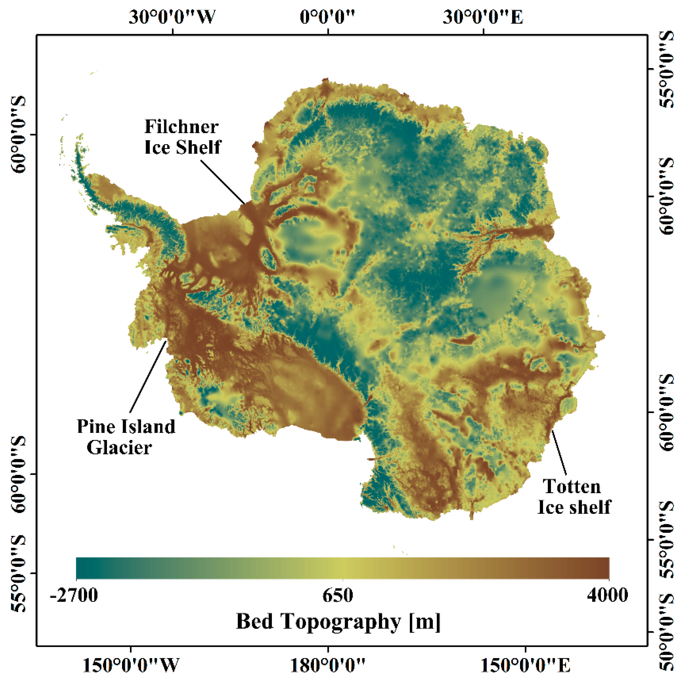
2.1. Study Area

Figure 1 shows the spatial distribution of the study area [41]. The training and testing data are situated on the Pine Island ice shelf, located in the southwestern region of Antarctica (Figure 2). This ice shelf has been experiencing prolonged periods of accelerated motion [42,43], with maximum velocities exceeding 4.5 km/yr [44]. Observations spanning several decades have revealed the retreat of the grounding line of the Pine Island ice shelf into the ice sheet [45]. Additionally, the presence of numerous crevasses on the ice shelf surface serves as evidence of intensified glacier movement [46]. The continuous acceleration of glacier motion and the occurrence of calving events leading to frequent changes in the calving front location provide a strong experimental basis for calving front extraction.

In order to verify the applicability of the model in other regions, we also selected the Totten Ice Shelf and the Filchner Ice Shelf as experimental areas. The Totten Ice Shelf, located in the east Antarctic, holds the equivalent of 3.5 m of global sea level rise [47]. The Filchner ice shelf, located in the west Antarctic, lies at the head of the Weddell Sea. The ice shelf is over 200 m thick [48]. The positions of the two ice shelves are shown in Figure 1.

2.2. Input Data

The Landsat series satellites, known for their moderate resolution, are commonly used as data sources for monitoring changes in Antarctic ice shelves [49,50,51,52,53,54]. Due to the linear nature of the calving front, datasets with moderate spatial resolution are necessary to ensure accurate results. In our study, we utilized the panchromatic bands from Landsat 7 and Landsat 8 which provide a spatial resolution of 15 m [55].

Table 1. Landsat Imagery Information.

Data	Path/Row	Series	Cloud Cover (%)
20130215	185/116	Landsat7	1.00
20140226	185/116	Landsat8	0.00
20150301	185/116	Landsat8	13.02
20160115	185/116	Landsat8	3.67
20170218	185/116	Landsat8	0.08
20180205	185/116	Landsat8	5.80
20190312	185/116	Landsat8	0.54
20200218	186/116	Landsat8	0.04
20210128	185/116	Landsat8	16.80
20220224	185/116	Landsat8	0.14
20130109	102/107	Landsat7	1.00
20140129	101/107	Landsat8	7.40
20150321	101/107	Landsat8	0.14
20160119	101/107	Landsat8	1.73
20170222	101/107	Landsat8	0.00
20180108	101/107	Landsat8	0.00
20190228	101/107	Landsat8	0.00
20200302	101/107	Landsat8	11.64
20210217	101/107	Landsat8	18.90
20220220	101/107	Landsat8	0.00

presents the specific details of the data used. Landsat is an Earth observation satellite program jointly administered by the U.S. Department of the Interior National Aeronautics and Space Administration (NASA) and the Department of Agriculture. The program’s first satellite was launched on 23 July 1972. The Landsat series satellites operate in near-polar circular orbits at an orbital altitude of 705 km, an orbital inclination of 98.2°, a revisit period of 16 days, and a satellite coverage range from 81°N to 81.5°S.

2.3. Methods

In this study, the automatic extraction of the calving front involves five main steps: (1) pre-processing of optical images, (2) model training and post-processing of results, (3) extraction of boundaries using edge detection operators, (4) accuracy evaluation, and (5) generalization analysis of the model (Figure 3). The pre-processing of optical images includes tasks such as image filling and cropping to enhance the efficiency of training. Image filling means expanding the edges of the image. The second step involves model training and parameter adjustment to determine the optimal number of network training iterations and batch size. Once the semantic segmentation of the image is completed using U²-Net, a binary result graph is obtained. Initially, some pixel blocks are inaccurately extracted and these blocks (with a size of less than 30,000 pixels) are reclassified based on proximity. To extract the precise location of the calving front, the Canny edge detection operator is employed. Two sets of indexes are used for accuracy evaluation: (1) binary classification metrics are employed to classify the results of network models and (2) the area enclosed by the two calving fronts divided by the average length of the front is used to evaluate the extraction results of the Canny operator. The average length of the front is calculated based on both automatic extraction and manual interpretation results. The calving front location was determined through visual interpretation using ArcGIS software. The interpretation standard is based on the difference in gray values between the ice shelf and the ocean in the image. The calving front is defined as the boundary between the ocean and land ice, including floating ice shelves and glacier tongues. However, it is important to note that the time intervals of similar products in the published dataset are not continuous. To accurately analyze the results obtained by the network, we require a continuous and reliable dataset with precise information. The training set used by the network model was obtained through visual interpretation and digitization using ArcGIS software; we consider the visual results as true knowledge for further analysis.

In the final step, the model’s generalization capability is tested by applying it to extract the calving front of the Filchner and Totten ice shelves.

2.3.1. Pre-Processing and Data Preparation

After selecting the area near the calving front and clipping the corresponding image, the final image size is 2922 × 2959 pixels while the training set size is 128 × 128 pixels. To maximize the utilization of information in the input image, particularly the pixel information at the edges, we performed an edge complement operation on the original image before training. This operation ensured that the length and width of the image were multiples of 128, resulting in an image size of 2944 × 3072 after edge complement. The training set here adopts three years of Landsat images in 2014, 2016, and 2018; the number after edge filling and clipping results in a final number of 1656 training samples. The Landsat image in 2019 was used as the test set with the number 552. The remaining Landsat data shown in Table 1 are the images used in the extraction of ice shelf (Pine Island, Totten, and Filchner) calving front location.

To expose the model to various situations of the calving front as much as possible within the limited training set, we implemented two steps. Firstly, considering the different orientations of the calving front across different ice shelves, we applied enhanced processing to the training samples, including rotation and mirroring of images. This approach enabled the model to learn the morphological characteristics of various calving front trends. Secondly, due to the varying acquisition times of satellite images and the resulting differences in illumination conditions between ice shelf and ocean locations, there were significant variations in image gray value and contrast. Therefore, the input image is rotated and mirrored and the brightness of pixel values is adjusted to expand the data set. Following these operations, the number of training samples increased from 1656 to 6624.

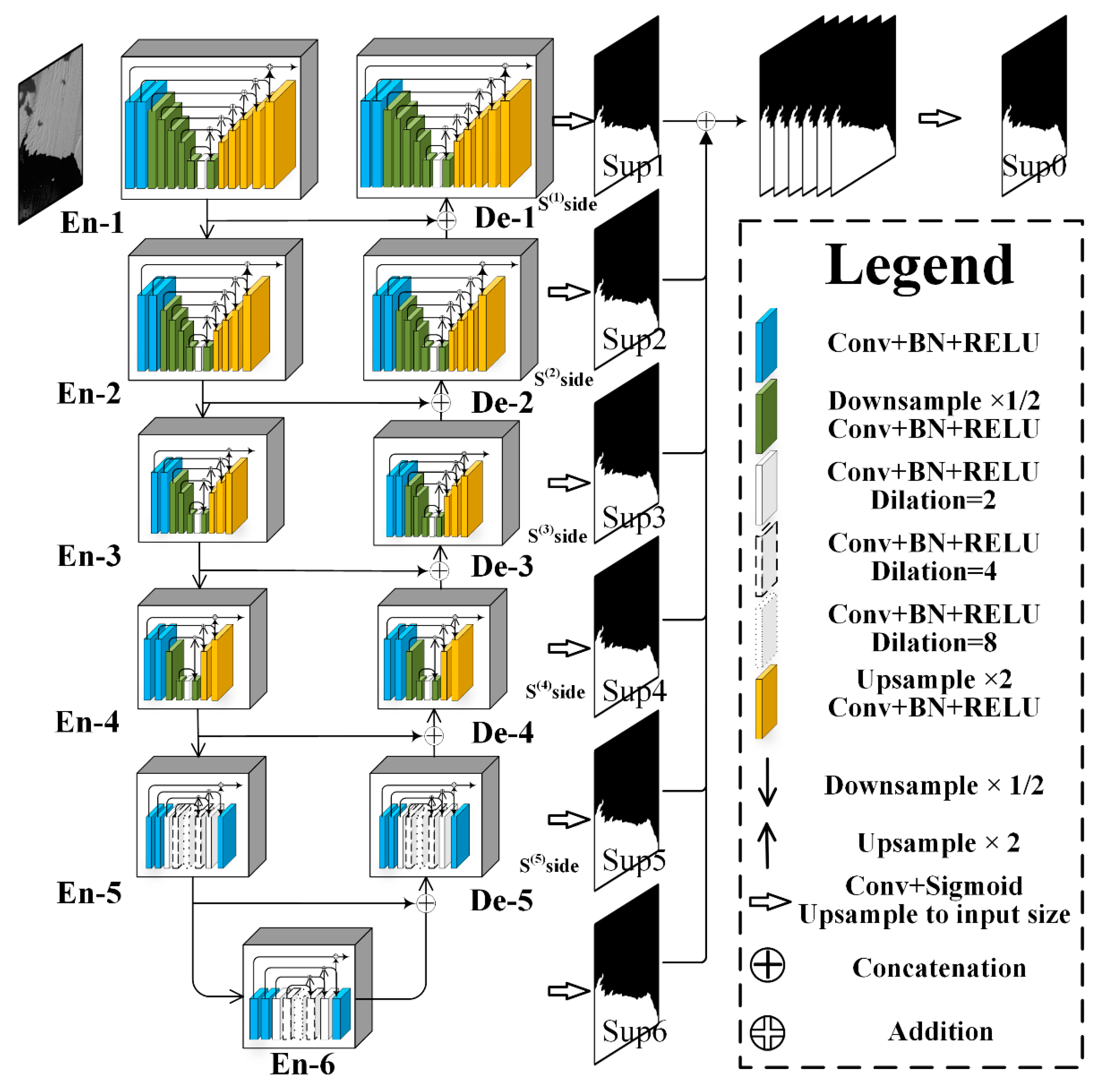
2.3.2. U²-Net Architecture and Post-Processing

U²-Net, a target detection model based on the traditional U-Net, is utilized in this study. It introduces a two-layer nested U-shaped structure (Figure 4) allowing for training the network from scratch without relying on pre-training models. Moreover, the model maintains high resolution as it becomes deeper while minimizing video memory overhead and computational requirements. Comparative experiments with multiple network models have demonstrated that U²-Net enhances accuracy, making it a suitable choice for extracting the features of the calving front [40,56].

The U²-Net model follows a U-shaped structure consisting of six encoders on the left and five decoders on the right. Each layer contains a small module with a U-shaped structure which is why it is referred to as ‘U².’ The encoding and decoding modules, represented as ‘En-’ and ‘De-’ in Figure 4, are the key features of the model. In Residual U-blocks (RSU) (Figure 5), various operations like convolution and down sampling can enhance the network’s ability to extract features. The residual connection effectively combines these multi-dimensional features, allowing RSU to improve network performance by integrating local details and high-level semantic information.

The model incorporates the multi-supervision algorithm to construct the objective function. It fuses feature maps from each layer and the final feature map, allowing both the network output and intermediate feature map fusion to be supervised. To expand the receptive field, the model utilizes dilation operations. Figure 6 demonstrates how adjusting the dilation parameter values can result in different receptive fields. This proves advantageous in studying the calving front as it expands the receptive field without significantly increasing computational requirements, thus improving image classification accuracy.

The classification of images by neural networks is performed pixel by pixel. Sometimes, misclassified pixels tend to cluster together. For instance, in the task of image classification where the goal is to extract the boundary line between an ice shelf and the ocean, the ideal classification outcome would assign a pixel value of 0 (black) to the ice shelf area and 255 (white) to the ocean area. However, in actual classification results, there may be clusters of different pixel types present in both the ice shelf and ocean areas. This interference can affect the subsequent edge extraction process which relies on detecting areas with the most significant changes in gray intensity. When different pixel types form clusters, they deviate from the gray values of the surrounding pixels. These small regions, after being processed by the edge extraction algorithm, create boundaries that are not the desired positions of interest. To address these issues, an empirical threshold processing technique is applied to the results of the neural network classification. The threshold was determined through multiple tests. We conducted tests with thresholds of 2000, 5000, 10,000, and 30,000. When the threshold was set at 30,000, it effectively eliminated misclassified pixel blocks. If the number of pixel blocks within a connected domain dropped below the threshold of 30,000 pixels, the classification result of the pixels within that domain was adjusted. This adjustment process resulted in a binary image with a distinct dividing line and eliminated any noise points. Finally, the Canny operator is employed to extract the dividing line and determine the position of the calving front.

2.3.3. Training Loss of U²-Net

According to Figure 3, the overall loss of the network can be expressed as [35]:

$$\mathrm{L}={\sum }_{\mathrm{m}=1}^6{\mathrm{w}}_{\mathrm{s}\mathrm{i}\mathrm{d}\mathrm{e}}^{\left(\mathrm{m}\right)}{\mathrm{l}}_{\mathrm{s}\mathrm{i}\mathrm{d}\mathrm{e}}^{\left(\mathrm{m}\right)}+{\mathrm{w}}_{\mathrm{f}\mathrm{u}\mathrm{s}\mathrm{e}}{\mathrm{l}}_{\mathrm{f}\mathrm{u}\mathrm{s}\mathrm{e}}$$

(1)

where ${\mathrm{l}}_{\mathrm{s}\mathrm{i}\mathrm{d}\mathrm{e}}^{\left(\mathrm{m}\right)}$ (as the Sup1, Sup2, · · ·, Sup6 in Figure 3) represents the loss of the side output saliency map ${\mathrm{S}}_{\mathrm{s}\mathrm{i}\mathrm{d}\mathrm{e}}^{\left(\mathrm{m}\right)}$ and ${\mathrm{l}}_{\mathrm{f}\mathrm{u}\mathrm{s}\mathrm{e}}$ (Sup7) is the loss of the final fusion output saliency map ${\mathrm{S}}_{\mathrm{f}\mathrm{u}\mathrm{s}\mathrm{e}}$. The ${\mathrm{w}}_{\mathrm{s}\mathrm{i}\mathrm{d}\mathrm{e}}^{\left(\mathrm{m}\right)}$ and ${\mathrm{w}}_{\mathrm{f}\mathrm{u}\mathrm{s}\mathrm{e}}$ are the weights of mentioned losses. For any $\mathrm{l}$, the binary crossentropy is used as follows [35]:

$$\mathrm{l}=-{\sum }_{(\mathrm{r},\mathrm{c})}^{(\mathrm{H},\mathrm{W})}[{\mathrm{P}}_{\mathrm{G}(\mathrm{r},\mathrm{c})}{\log \mathrm{P}}_{\mathrm{S}(\mathrm{r},\mathrm{c})}+(1-{\mathrm{P}}_{\mathrm{G}(\mathrm{r},\mathrm{c})})\log (1-{\mathrm{P}}_{\mathrm{S}(\mathrm{r},\mathrm{c})})]$$

(2)

where (r, c) and (H, W) represent coordinates and dimensions, respectively. ${\mathrm{P}}_{\mathrm{G}(\mathrm{r},\mathrm{c})}$ and ${\mathrm{P}}_{\mathrm{S}(\mathrm{r},\mathrm{c})}$ denote the ground truth and the probability of prediction. In addition, the fusion output ${\mathrm{l}}_{\mathrm{f}\mathrm{u}\mathrm{s}\mathrm{e}}$ is considered as the final result.

2.3.4. Training Strategy

In this section, we followed the hyperparameter settings of the original networks; the specific parameters can be found in

Table 2. Hyperparameter settings of the original networks.

Index	FCN	U-Net	U2-Net
Learning rate	0.001
Epoch	800
Batch size	8	8	4
Adam optimizer	SGD (momentum = 0.7))	Adam (betas = (0.9, 0.999), eps = 1 × 10−8, weight decay = 0)	Adam (betas = (0.9, 0.999), eps = 1 × 10−8, weight decay = 0)
Loss function	Binary Cross Entropy Loss

.

To ensure fairness, we used a 128 × 128 size input and set the epoch to 800 during the training process. The training was conducted on an AMD R7-5800x platform with a 3070ti GPU of 8GB memory. The code is implemented through pycharm software and the framework is pytorch.

Table 3. The parameters of the networks structure.

	En_1	En_2	En_3	En_4	En_5	En_6	De_5	De_4	De_3	De_2	De_1
U2-Net	I:3	I:64	I:128	I:256	I:512	I:512	I:1024	I:1024	I:512	I:256	I:128
	M:32	M:32	M:64	M:128	M:256	M:256	M:256	M:128	M:64	M:32	M:16
	O:64	O:128	O:256	O:512	O:512	O:512	O:512	O:256	O:128	O:64	O:64
U-Net	I:3	I:64	I:128	I:256	I:512	I:512	I:1024	I:1024	I:512	I:256	I:128
	M:64	M:128	M:256	M:512	M:512	M:512	M:512	M:256	M:128	M:64	M:64
	O:64	O:128	O:256	O:512	O:512	O:512	O:512	O:256	O:128	O:64	O:64
FCN	I:3	I:64	I:128	I:256	I:512						I:512
	O:64	O:128	O:256	O:512	O:512						O:256

presents the network model structure parameters to better explain the differences among the three. The feature graph channel numbers for the encoding and decoding parts of the three networks are included to distinguish their variations. “I”, “M”, and “O” represent the number of input channels, intermediate channels, and output channels for each block. “En_i” and “De_j” denote the encoder and decoder phases, respectively. Additionally, there is a maximum pooling between each “En_i”.

2.3.5. Accuracy Assessment

This paper proposes three methods for evaluating accuracy in image classification. The first method is the conventional index of neural network evaluation which includes precision, recall, F1, and IOU. These metrics can be used to compare the performance of different models. The second method refers to the indexes of accuracy evaluation used by relevant scholars [54]. The third evaluation criterion involves assessing the results obtained after applying the Canny operator to extract the calving front. The specific calculation process for the above two evaluation methods is as follows:

Semantic segmentation evaluation standards were used to discuss different network models, including Precision, Recall, F1, and IOU [51]. These metrics were calculated as follows:

$$\mathrm{P}\mathrm{r}\mathrm{e}\mathrm{c}\mathrm{i}\mathrm{s}\mathrm{i}\mathrm{o}\mathrm{n}=\mathrm{T}\mathrm{P}/(\mathrm{T}\mathrm{P}+\mathrm{F}\mathrm{P})$$

(3)

$$\mathrm{R}\mathrm{e}\mathrm{c}\mathrm{a}\mathrm{l}\mathrm{l}=\mathrm{T}\mathrm{P}/(\mathrm{T}\mathrm{P}+\mathrm{F}\mathrm{N})$$

(4)

$$\mathrm{F}1=2\ast \mathrm{T}\mathrm{P}/(2\mathrm{T}\mathrm{P}+\mathrm{F}\mathrm{N}+\mathrm{F}\mathrm{P})$$

(5)

$$\mathrm{I}\mathrm{O}\mathrm{U}=\mathrm{T}\mathrm{P}/(\mathrm{T}\mathrm{P}+\mathrm{F}\mathrm{P}+\mathrm{F}\mathrm{N})$$

(6)

where TP (true positive) represents the region of the ice shelf correctly extracted and TN (true negative) represents the ocean area correctly extracted. FP (false positive) represents the area of the ice shelf that was incorrectly extracted. FN (false negative) represents the ocean area that was incorrectly extracted.

These matrix elements will also be used to compute performance metrics for the neural networks. The calculations are as follows:

(1)

Accuracy (AC): This is an evaluation index for the network model which is used to measure the accuracy of the network for semantic segmentation. The accuracy of the model is defined as the proportion of correctly classified pixels in the classification result. The AC_mod is computed as [58]:

$${\mathrm{A}\mathrm{C}}_{\mathrm{m}\mathrm{o}\mathrm{d}}=\frac{\mathrm{T}\mathrm{P}+\mathrm{T}\mathrm{N}}{\mathrm{T}\mathrm{P}+\mathrm{T}\mathrm{N}+\mathrm{F}\mathrm{P}+\mathrm{F}\mathrm{N}}$$

(7)

(2)

Cohen’s Kappa Coefficient (k): This parameter is used to measure the degree of consistency between manual visual interpretation and model classification results. The higher this index is, the closer the model result is to the real classification situation which from manual extraction. The specific calculation method is as follows [58]:

$$\mathrm{k}=1-\frac{1-{\mathrm{A}\mathrm{C}}_{\mathrm{m}\mathrm{o}\mathrm{d}}}{1-{\mathrm{A}\mathrm{C}}_{\mathrm{r}\mathrm{d}}}$$

(8)

$${\mathrm{A}\mathrm{C}}_{\mathrm{r}\mathrm{d}}=\frac{\left(\mathrm{T}\mathrm{P}+\mathrm{F}\mathrm{N}\right)\times \left(\mathrm{T}\mathrm{P}+\mathrm{F}\mathrm{P}\right)+(\mathrm{T}\mathrm{N}+\mathrm{F}\mathrm{P})\times (\mathrm{T}\mathrm{N}+\mathrm{F}\mathrm{N})}{{(\mathrm{T}\mathrm{P}+\mathrm{T}\mathrm{N}+\mathrm{F}\mathrm{P}+\mathrm{F}\mathrm{N})}^2}$$

(9)

When evaluating the accuracy of the calving front extracted by the Canny operator compared with the results obtained by visual interpretation, we decided not to use the index of accuracy evaluation commonly used for neural network results. This is because there is typically a difference of 1~3 pixels between the extracted calving front and the visually interpreted results. Such differences are considered extremely poor results in evaluation systems that prioritize parameters like F1 or IOU. However, these evaluation criteria are not meaningful for the extraction results of linear features. The small pixel difference between the extracted result and the actual result can be accepted. Therefore, we propose using an area divided by the length to calculate the extraction accuracy of the calving front. In this context, the area refers to the irregular figure enclosed between the actual calving front and the extracted calving front while the length refers to the average value of the actual length and the extracted length of the calving front.

3. Results and Discussion

The dynamic changes in the calving front are closely linked to ice sheet mass loss, making it important to have a continuous and automated method for extracting calving fronts. In recent research, there has been a growing interest in using convolutional neural networks for interpreting remote-sensing images, particularly in the field of semantic segmentation. In this paper, we conducted experiments using three convolutional neural network models: FCN, U-Net, and U²-Net.

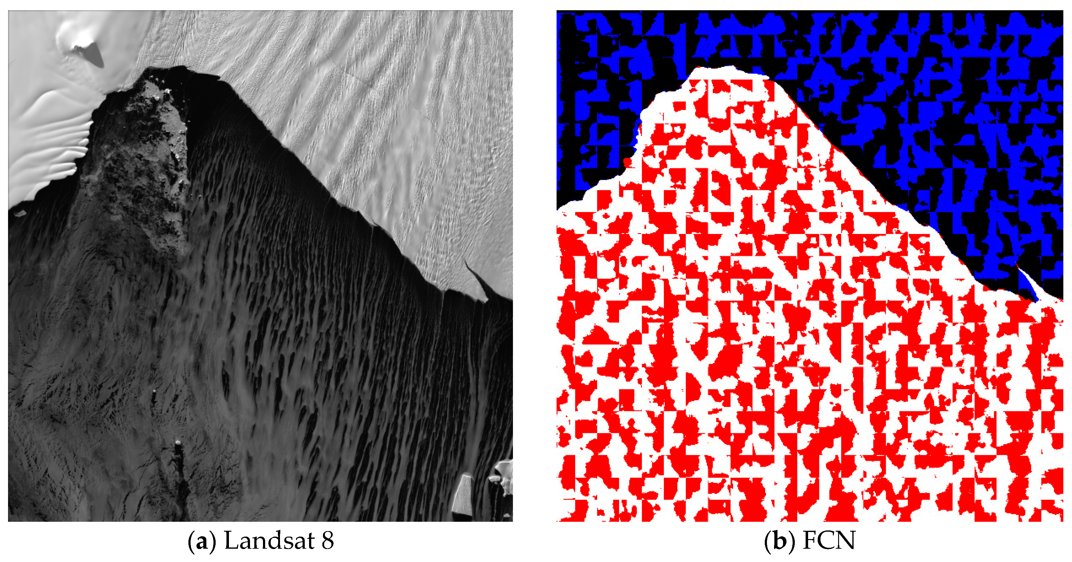
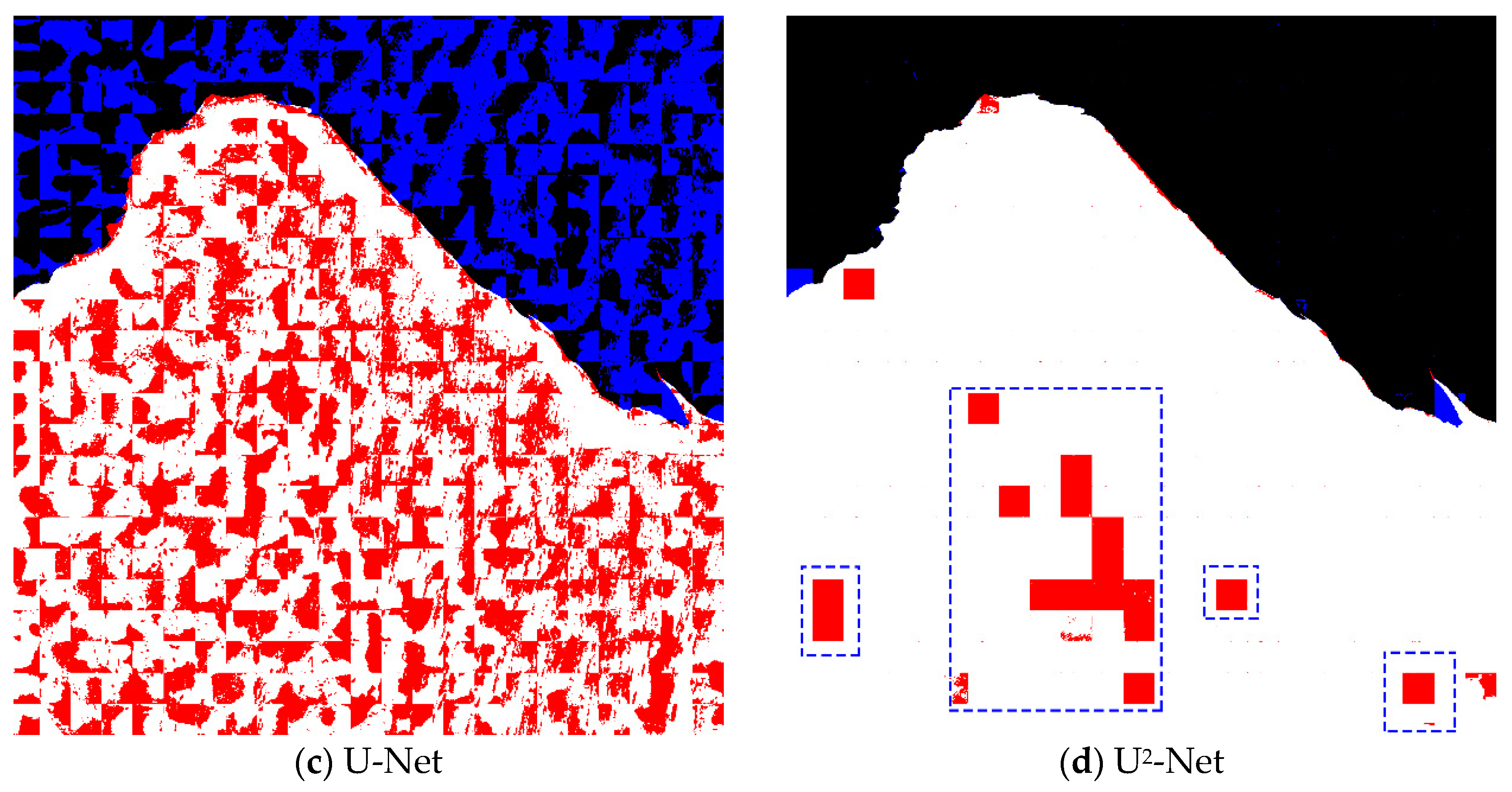
3.1. Comparison of Results

The results (Figure 7) obtained from FCN and U-Net indicate that these two types of neural networks struggle to accurately extract the calving front. However, U²-Net successfully reveals the position of the calving front, albeit with some misclassified pixel blocks (highlighted in the blue dotted line frame in Figure 7d). These pixel blocks can be eliminated through post-processing by focusing on these areas. The aforementioned results can be attributed to two main factors: (1) U²-Net utilizes a multi-supervision algorithm to construct the objective function, which involves the fusion of the feature map from each layer with the final feature map. This enables supervision of the network output and the intermediate fusion feature map. (2) The application of dilation in U²-Net enhances the receptive field of the network, allowing the model to comprehensively consider the partial context of each pixel during the classification process.

Table 4. Comparison of evaluation indexes of extraction result of calving front.

Model	FCN	U-Net	U2-Net
Precision (%)	69.04	66.97	99.43
Recall (%)	55.17	59.47	94.54
F1 (%)	61.33	63.00	96.93
IOU (%)	44.23	45.98	94.04
ACmod	54.72	54.53	96.10
k	8.32	4.58	91.59

The bold entities represent that the model performs optimally under the corresponding parameters.

presents the performance of FCN, U-Net, and U²-Net in various precision indexes. While precision and recall values alone cannot fully capture the strengths and weaknesses of the network architecture, it is more reasonable to evaluate using the reconciled average value F1 which combines both metrics. Comparing with FCN, U-Net shows an increase of 1.67% in F1 and 1.75% in IOU. However, both models have limitations in overall classification effectiveness. Figure 7b,c demonstrates that although the boundary between the ice shelf and the ocean can be blurred, it does not meet the requirements for subsequent edge detection operations. On the other hand, U²-Net performs significantly better than the previous two models in the case of AC_mod. The performance of Cohen’s kappa Coefficient (k) suggests that U²-Net is more suitable for classifying ice shelf regions.

Compared with the extraction results of the previous two models, U²-Net demonstrates superior performance. It achieves high accuracy in all six evaluation indexes (precision, recall, F1, IOU, AC_mod, and k), with values exceeding 90%. This is a significant improvement compared to the previous two networks. The excellent extraction results of U²-Net can be attributed to its unique double-layer ‘U’ structure and the generation of six saliency probability maps from different sides, which are then combined. The model effectively extracts multi-scale features at each stage. Therefore, this paper selects U²-Net for processing subsequent data as it demonstrates better extraction capabilities for the calving front of the ice shelf.

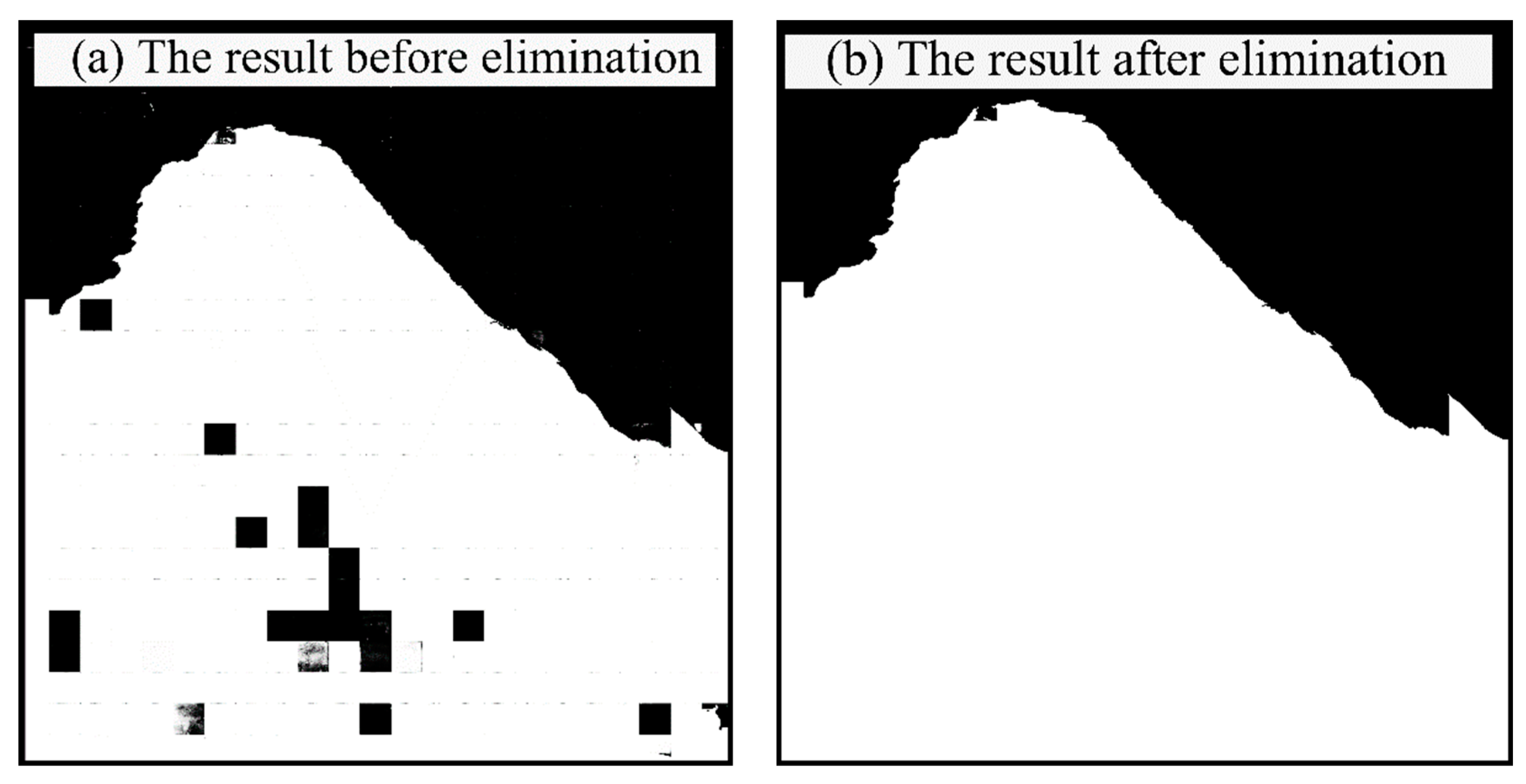
3.2. U²-Net Result Post-Processing and Edge Extraction

In the results of calving front location by the neural network, there are scattered distribution area pixel aggregations in individual positions (the part in the blue dotted line box in Figure 7d). These results do not affect the visual interpretation results. However, in the future, we need to use the Canny operator to automatically extract the location of the calving front. If these wrongly extracted small regions are not removed, edge detection will extract the edge of these positions, thus affecting the final result.

To remove pixel blocks in a small area, we adopt the threshold method. First, we roughly estimate that the number of pixels at the location of the minimum pixel block aggregation is about 2000. Furthermore, we estimate that the number of black pixel blocks in the maximum range of the blue dotted line box in Figure 7d is between 20,000–30,000. Therefore, we set the threshold as 30,000. If the number of clustered pixel blocks is less than 30,000, the gray value (white) of surrounding pixel blocks will be assigned. For U2-Net classification results, a threshold of 30,000 is sufficient to remove pixels of incorrect classification. Once the setting is complete, subsequent batch processing operations can be performed. After performing the above operations, we obtained the comparison of results before and after the elimination of small areas, as shown in Figure 8.

The results after elimination are shown in Figure 8b. In the figure, the black pixel block represents the position of the ice shelf while the white pixel block represents the position of the ocean; the dividing line between the two is the position of the calving front. Based on this, edge detection using the Canny operator is performed. To further verify the accuracy of the edge detection operator extraction, we compared the results of Canny extraction with manual extraction. By calculating the ratio of the area enclosed by the lines (automatic extraction and manual extraction) to the average length of the calving front, we calculated the error (in terms of number of pixels) of the automatic extraction results.

Figure 9 presents the outcomes of calving front extraction using a combination of neural networks and artificial visual interpretation. To assess the accuracy of the deep learning extraction results, this study calculates the ratio of the area between the two lines to the average length of the calving front. This ratio serves as a measure of the automatic extraction accuracy. The precision value obtained for the calving front shown in Figure 9 is 3.89 pixels. Considering the spatial resolution of the image, which is 15 m, the precision of extracting the Pine Island ice shelf calving front is determined to be 58.35 m.

According to

Table 5. Accuracy comparison of U²-Net and other publicly published calving front location extraction results.

Author	Year	Method	Accuracy	Data
Celia A. Baumhoer [34]	2019	modified U-Net	108 m	Sentinel-1
Yara Mohajerani [32]	2019	modified U-Net	92.5 m	Landsat 5; Landsat 7; Landsat 8.
Enze Zhang [60]	2021	combination of histogram normalization and DRN-DeepLabv3+	86 m	Landsat-8; Sentinel-2; Envisat; ALOS-1; TerraSAR-X; Sentinel-1; ALOS-2.
Konrad Heidler [59]	2022	HED-UNet	80.5 m	Sentinel-1

, the HED-Net model proposed by Konrad Heidler et al. (2022) [59] achieves the highest accuracy, with a final accuracy of 80.5 m using Sentinel-1 satellite data. In contrast to the previous method, we utilized Landsat images which do not contain speckle noise like SAR images. SAR layover and shadowing can be caused by the acquisition geometry and topography of the monitored area. On the other hand, optical images allow even non-experts to easily distinguish calving fronts. Yara Mohajerani et al. (2019) [32] also employed Landsat images but in this paper, we utilized the U²-Net model which achieved a better accuracy of 58.35 m in calving front location extraction. The U²-Net model demonstrates stronger competitiveness.

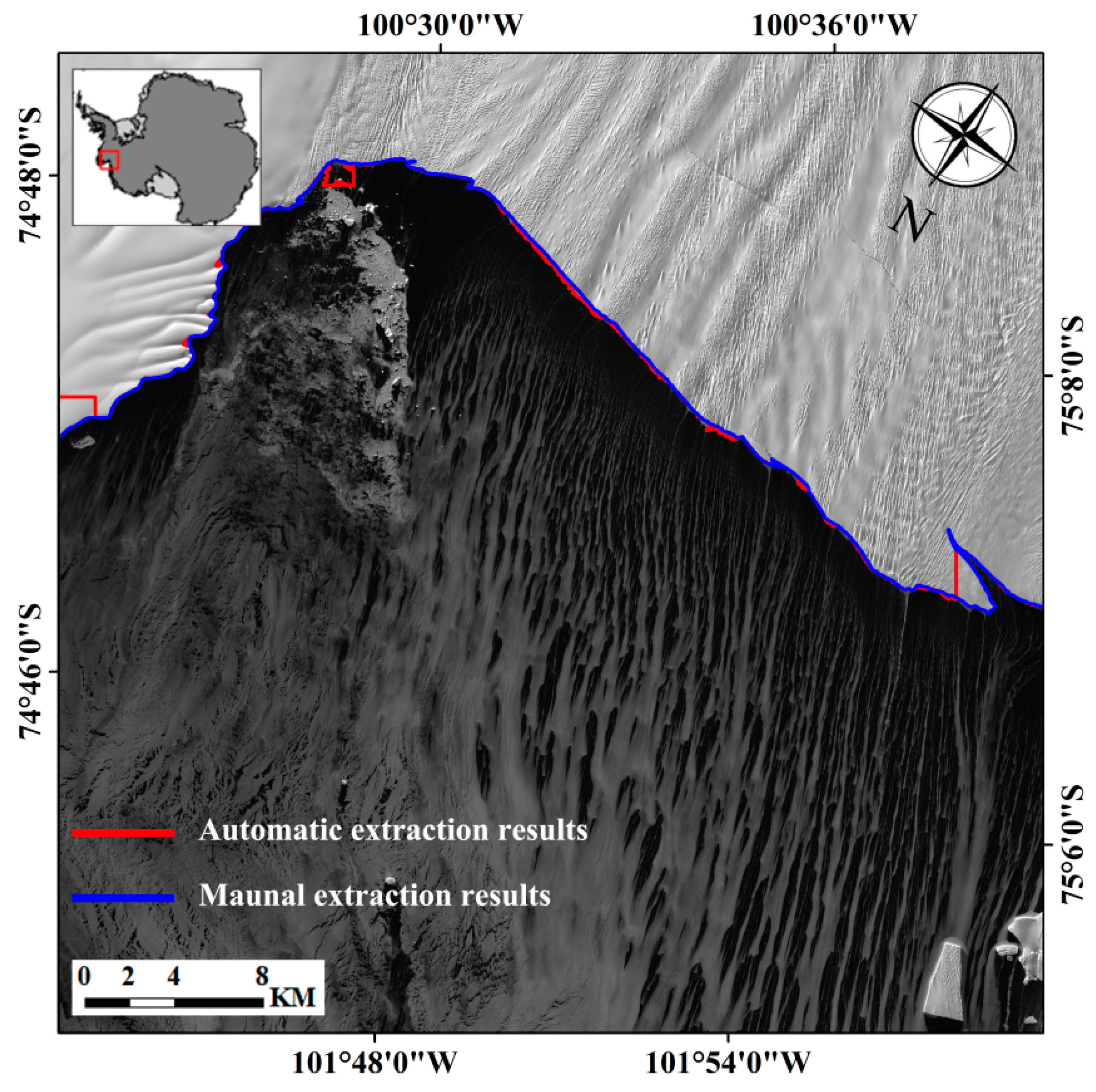
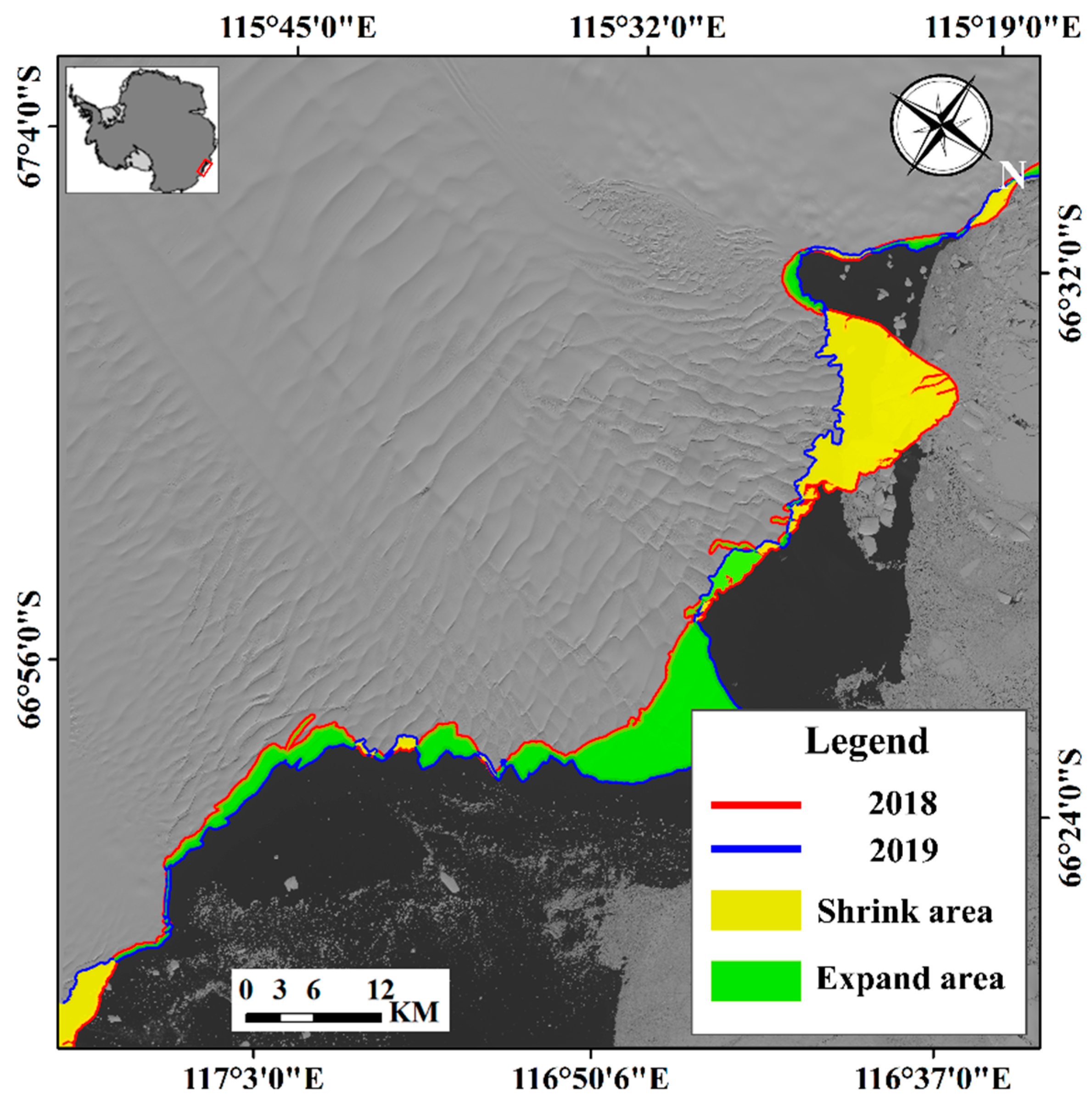
3.3. Model Generalization

After the above discussion, the combination of U²-Net and the Canny edge operator can be used to extract the calving front of the ice shelf. In order to evaluate the applicability of this method to other Antarctic ice shelves, two additional test areas were selected.

Figure 10 illustrates the changes in the calving front of Totten and Filchner ice shelves over the past decade. To facilitate a clearer comparison of the changes between the two ice shelves, we present the numerical changes in the calving front of each ice shelf.

The calving front location of the Totten Ice Shelf in 2018 and 2019 are represented by the red and blue lines in Figure 11, respectively. The yellow areas indicate the retreat of the ice shelf compared to the previous year while the green areas represent its expansion. To calculate the overall change in the calving front, we statistically analyzed the receding/expanding area near the front line. Negative values denote the receding range while positive values indicate the expanding range. The sum of these values provides the final receding/expanding range. This range is then divided by the average length of the two front lines to determine the change value.

Figure 12 illustrates the changes in the calving front of the Filchner and Totten Ice Shelves. Positive values signify the forward distance of the front line compared to the previous year while negative values indicate the retreat distance. Based on the data presented in Figure 12, it is evident that the Filchner ice shelf experienced more significant changes, reaching a maximum expansion distance of 3532.84 m in 2014–2015. The most stable year was 2018–2019, with the calving front advancing by 217.16 m. In comparison, the Totten Ice Shelf exhibited greater stability, with a maximum distance change of 715.92 m in 2014–2015. The year with the smallest change was 2021–2022, during which the calving front advanced by 14.62 m.

4. Conclusions

Based on the comparison of segmentation results, U²-Net has been found to be more suitable for remote sensing image interpretation in calving front extraction. The effectiveness of the models was verified by comparing the extraction results of the Pine Island Ice Shelf with visual interpretation. Expanding on the impressive performance of U²-Net in calving front extraction, this study successfully applied the model to the Filchner and Totten Ice Shelves for a period of almost 10 years, resulting in positive outcomes. The specific research findings can be summarized as follows:

(1)

The comparison of extraction results of the Pine Island Ice Shelf using FCN and U-Net demonstrated that U-Net, with its inclusion of a ‘skip’ operation in the network architecture, effectively integrates both low-resolution and high-resolution information. This integration leads to enhanced accuracy in F1 and IOU metrics. Specifically, there was a 1.67 percentage point increase in F1 and a 1.42 percentage point increase in IOU;

(2)

In comparison to the previous two models, U²-Net demonstrated the highest accuracy. This can be attributed to its utilization of the ‘U’ structure which enables the extraction of multi-scale features at each stage. Additionally, the model employed the multi-supervision algorithm to construct the objective function. By fusing feature maps from each layer and the final feature map, the network output and intermediate feature map fusion were both supervised, leading to a significant enhancement in classification accuracy. The evaluation indexes of the model indicated an accuracy above 90%, highlighting its suitability for semantic segmentation of Ice Shelves and oceans;

(3)

In order to further analyze the differences between the models in the Ice Shelf region, their performance was compared in terms of AC_mod and k values. The findings showed that the AC_mod value of U²-Net was 41.38 percentage points higher than U-Net and 41.57 percentage points higher than FCN. Additionally, the U²-Net model demonstrated superior performance in terms of the k value, indicating distinct advantages in classifying Ice Shelf regions at various levels;

(4)

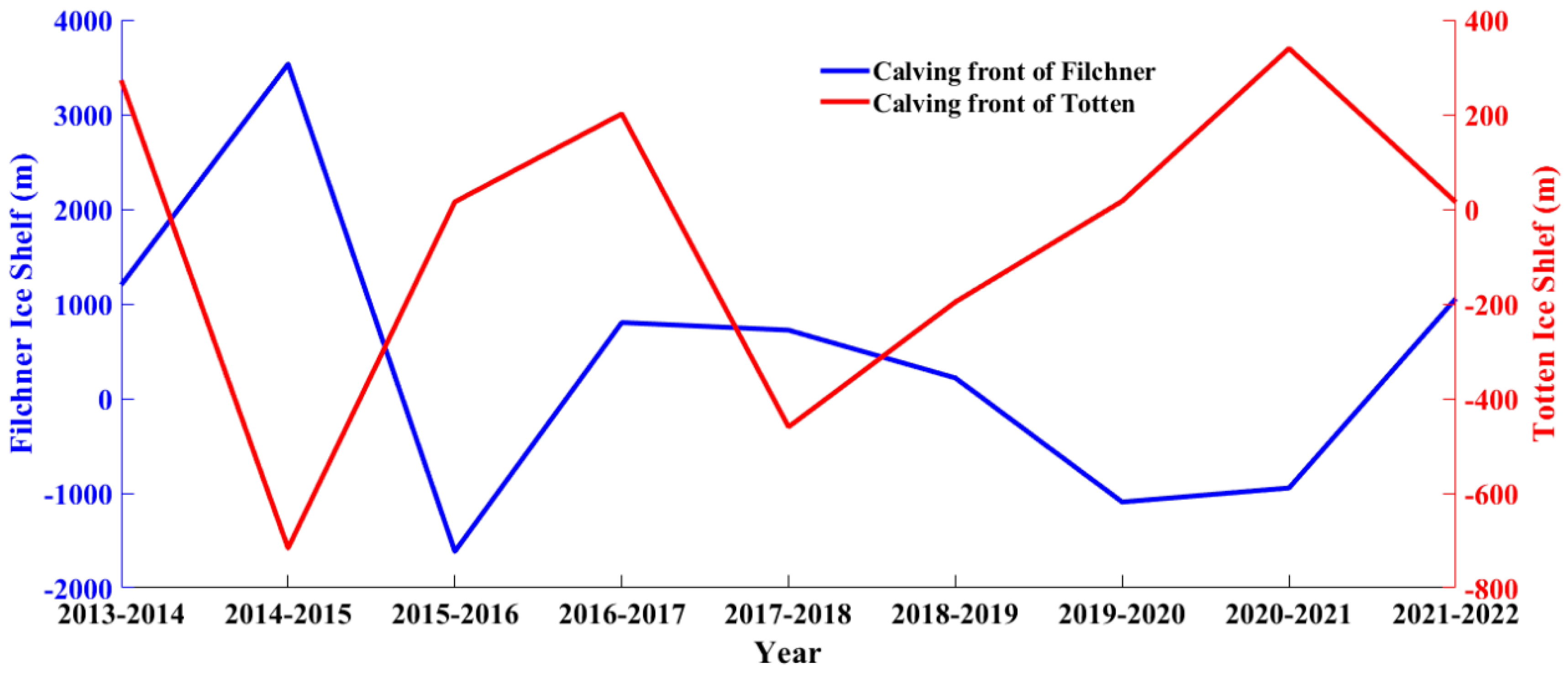
The U²-Net model demonstrates strong generalization capabilities and has been successfully applied to analyze the Totten and Filchner Ice Shelves. This analysis allowed for the extraction of calving front changes over the past 10 years. The results revealed that the Filchner Ice Shelf exhibited more pronounced changes compared to the Totten Ice Shelf. Specifically, the calving front of the Filchner Ice Shelf advanced by 3532.84 m during the period of 2014–2015 while the maximum advancement of the Totten Ice Shelf occurred between 2020 and 2021, reaching 339.63 m;

(5)

By comparing the accuracy of each model in extracting the calving front location in this paper, it was found that U²-Net is more suitable for this purpose. Subsequent research can optimize the U²-Net model to improve the efficiency and accuracy of calving front extraction. Moreover, the method proposed in this study can also be applied to monitor similar disasters. For instance, in the case of natural disasters in India where the sudden acceleration of mountain glaciers leads to the formation of cracks on the surface that gradually expand over time, this paper’s method enables the numerical representation of such changes. This facilitates the analysis of specific change data to evaluate potential risks.

References

1. Bondzio, J.H.; Seroussi, H.; Morlighem, M.; Kleiner, T.; Rückamp, M.; Humbert, A.; Larour, E.Y. Modelling calving front dynamics using a level-set method: Application to Jakobshavn Isbræ, West Greenland. Cryosphere 2016, 10, 497–510. [Google Scholar] [CrossRef]
2. Rosier, S.H.; Gudmundsson, G.H. Exploring mechanisms responsible for tidal modulation in flow of the Filchner–Ronne Ice Shelf. Cryosphere 2020, 14, 17–37. [Google Scholar] [CrossRef]
3. Müller, U.; Sandhäger, H.; Sievers, J.; Blindow, N. Glacio-kinematic analysis of ERS-1/2 SAR data of the Antarctic ice shelf Ekströmisen and the adjoining inland ice sheet. Polarforschung 2000, 67, 15–26. [Google Scholar]
4. Nicholls, K.W.; Østerhus, S.; Makinson, K.; Gammelsrød, T.; Fahrbach, E. Ice-ocean processes over the continental shelf of the southern Weddell Sea, Antarctica: A review. Rev. Geophys. 2009, 47. [Google Scholar] [CrossRef]
5. McCormack, F.; Roberts, J.; Gwyther, D.; Morlighem, M.; Pelle, T.; Galton-Fenzi, B.K. The impact of variable ocean temperatures on Totten Glacier stability and discharge. Geophys. Res. Lett. 2021, 48, e2020GL091790. [Google Scholar] [CrossRef]
6. Gens, R. Remote sensing of coastlines: Detection, extraction and monitoring. Int. J. Remote Sens. 2010, 31, 1819–1836. [Google Scholar] [CrossRef]
7. Furst, J.J.; Durand, G.; Gillet-Chaulet, F.; Tavard, L.; Rankl, M.; Braun, M.; Gagliardini, O. The safety band of Antarctic ice shelves. Nat. Clim. Change 2016, 6, 479–482. [Google Scholar] [CrossRef]
8. Sakakibara, D.; Sugiyama, S. Ice-front variations and speed changes of calving glaciers in the Southern Patagonia Icefield from 1984 to 2011. J. Geophys. Res. Earth Surf. 2014, 119, 2541–2554. [Google Scholar] [CrossRef]
9. Wuite, J.; Nagler, T.; Gourmelen, N.; Escorihuela, M.J.; Hogg, A.E.; Drinkwater, M.R. Sub-annual calving front migration, area change and calving rates from swath mode CryoSat-2 altimetry, on Filchner-Ronne Ice Shelf, Antarctica. Remote Sens. 2019, 11, 2761. [Google Scholar] [CrossRef]
10. Baumhoer, C.A.; Dietz, A.J.; Dech, S.; Kuenzer, C. Remote sensing of antarctic glacier and ice-shelf front dynamics—A review. Remote Sens. 2018, 10, 1445. [Google Scholar]
11. Mason, D.C.; Davenport, I.J. Accurate and efficient determination of the shoreline in ERS-1 SAR images. IEEE Trans. Geosci. Remote Sens. 1996, 34, 1243–1253. [Google Scholar] [CrossRef]
12. Modava, M.; Akbarizadeh, G. Coastline extraction from SAR images using spatial fuzzy clustering and the active contour method. Int. J. Remote Sens. 2017, 38, 355–370. [Google Scholar] [CrossRef]
13. Liu, H.; Jezek, K.C. A complete high-resolution coastline of Antarctica extracted from orthorectified Radarsat SAR imagery. Photogramm. Eng. Remote Sens. 2004, 70, 605–616. [Google Scholar] [CrossRef]
14. Alonso, M.T.; López-Martínez, C.; Mallorquí, J.J.; Salembier, P. Edge enhancement algorithm based on the wavelet transform for automatic edge detection in SAR images. IEEE Trans. Geosci. Remote Sens. 2010, 49, 222–235. [Google Scholar] [CrossRef]
15. Yuan, L.; Xu, X. Adaptive image edge detection algorithm based on canny operator. In Proceedings of the 2015 4th International Conference on Advanced Information Technology and Sensor Application (AITS), Harbin, China, 21–25 August 2015; IEEE: Piscataway, NJ, USA, 2015; pp. 28–31. [Google Scholar]
16. Deng, C.-X.; Wang, G.-B.; Yang, X.-R. Image edge detection algorithm based on improved canny operator. In Proceedings of the 2013 International Conference on Wavelet Analysis and Pattern Recognition, Tianjin, China, 14–17 July 2013; IEEE: Piscataway, NJ, USA, 2013; pp. 168–172. [Google Scholar]
17. Gao, W.; Zhang, X.; Yang, L.; Liu, H. An improved Sobel edge detection. In Proceedings of the 2010 3rd International Conference on Computer Science and Information Technology, Chengdu, China, 9–11 July 2010; IEEE: Piscataway, NJ, USA, 2010; Volume 5, pp. 67–71. [Google Scholar]
18. Chen, G.; Jiang, Z.; Kamruzzaman, M. Radar remote sensing image retrieval algorithm based on improved Sobel operator. J. Vis. Commun. Image Represent. 2020, 71, 102720. [Google Scholar] [CrossRef]
19. Seale, A.; Christoffersen, P.; Mugford, R.I.; O’Leary, M. Ocean forcing of the Greenland Ice Sheet: Calving fronts and patterns of retreat identified by automatic satellite monitoring of eastern outlet glaciers. J. Geophys. Res. Earth Surf. 2011, 116. [Google Scholar] [CrossRef]
20. LeCun, Y.; Bengio, Y.; Hinton, G. Deep learning. Nature 2015, 521, 436–444. [Google Scholar]
21. Zhu, X.X.; Tuia, D.; Mou, L.; Xia, G.-S.; Zhang, L.; Xu, F.; Fraundorfer, F. Deep learning in remote sensing: A comprehensive review and list of resources. IEEE Geosci. Remote Sens. Mag. 2017, 5, 8–36. [Google Scholar] [CrossRef]
22. Ambekar, S.; Tafuro, M.; Ankit, A.; der Mast, D.V.; Alence, M.; Athanasiadis, C. SKDCGN: Source-free Knowledge Distillation of Counterfactual Generative Networks Using cGANs. In Proceedings of the European Conference on Computer Vision, Tel Aviv, Israel, 23–27 October 2022; Springer: Berlin/Heidelberg, Germany, 2022; pp. 679–693. [Google Scholar]
23. Li, Y.; Zhang, H.; Xue, X.; Jiang, Y.; Shen, Q. Deep learning for remote sensing image classification: A survey. Wiley Interdiscip. Rev. Data Min. Knowl. Discov. 2018, 8, e1264. [Google Scholar] [CrossRef]
24. Sun, S.; Lu, Z.; Liu, W.; Hu, W.; Li, R. Shipnet for semantic segmentation on vhr maritime imagery. In Proceedings of the IGARSS 2018—2018 IEEE International Geoscience and Remote Sensing Symposium, Valencia, Spain, 23–27 July 2018; IEEE: Piscataway, NJ, USA, 2018; pp. 6911–6914. [Google Scholar]
25. Krizhevsky, A.; Sutskever, I.; Hinton, G.E. Imagenet classification with deep convolutional neural networks. Commun. ACM 2017, 60, 84–90. [Google Scholar] [CrossRef]
26. Xu, Y.; Du, J.; Dai, L.-R.; Lee, C.-H. A regression approach to speech enhancement based on deep neural networks. IEEE/ACM Trans. Audio Speech Lang. Process. 2014, 23, 7–19. [Google Scholar] [CrossRef]
27. Collobert, R.; Weston, J. A unified architecture for natural language processing: Deep neural networks with multitask learning. In Proceedings of the 25th International Conference on Machine Learning, Helsinki, Finland, 5–9 July 2008; pp. 160–167. [Google Scholar]
28. Liu, H.; Jezek, K. Automated extraction of coastline from satellite imagery by integrating Canny edge detection and locally adaptive thresholding methods. Int. J. Remote Sens. 2004, 25, 937–958. [Google Scholar] [CrossRef]
29. Leigh, S.; Wang, Z.; Clausi, D.A. Automated ice–water classification using dual polarization SAR satellite imagery. IEEE Trans. Geosci. Remote Sens. 2013, 52, 5529–5539. [Google Scholar] [CrossRef]
30. Kaushik, S.; Singh, T.; Joshi, P.; Dietz, A.J. Automated mapping of glacial lakes using multisource remote sensing data and deep convolutional neural network. Int. J. Appl. Earth Obs. Geoinf. 2022, 115, 103085. [Google Scholar]
31. Tuckett, P.A.; Ely, J.C.; Sole, A.J.; Lea, J.M.; Livingstone, S.J.; Jones, J.M.; van Wessem, J.M. Automated mapping of the seasonal evolution of surface meltwater and its links to climate on the Amery Ice Shelf, Antarctica. Cryosphere 2021, 15, 5785–5804. [Google Scholar]
32. Mohajerani, Y.; Wood, M.; Velicogna, I.; Rignot, E. Detection of glacier calving margins with convolutional neural networks: A case study. Remote Sens. 2019, 11, 74. [Google Scholar] [CrossRef]
33. Zhang, E.; Liu, L.; Huang, L. Automatically delineating the calving front of Jakobshavn Isbræ from multitemporal TerraSAR-X images: A deep learning approach. Cryosphere 2019, 13, 1729–1741. [Google Scholar] [CrossRef]
34. Baumhoer, C.A.; Dietz, A.J.; Kneisel, C.; Kuenzer, C. Automated extraction of antarctic glacier and ice shelf fronts from sentinel-1 imagery using deep learning. Remote Sens. 2019, 11, 2529. [Google Scholar] [CrossRef]
35. Qin, X.; Zhang, Z.; Huang, C.; Dehghan, M.; Zaiane, O.R.; Jagersand, M. U2-Net: Going deeper with nested U-structure for salient object detection. Pattern Recognit. 2020, 106, 107404. [Google Scholar]
36. Chen, B.; Liu, Y.; Zhang, Z.; Lu, G.; Kong, A.W.K. Transattunet: Multi-level attention-guided u-net with transformer for medical image segmentation. arXiv 2021, arXiv:2107.05274. [Google Scholar] [CrossRef]
37. Siddique, N.; Paheding, S.; Elkin, C.P.; Devabhaktuni, V. U-net and its variants for medical image segmentation: A review of theory and applications. IEEE Access 2021, 9, 82031–82057. [Google Scholar]
38. Yin, X.-X.; Sun, L.; Fu, Y.; Lu, R.; Zhang, Y. U-Net-Based Medical Image Segmentation. J. Healthc. Eng. 2022, 2022, 4189781. [Google Scholar] [PubMed]
39. Wei, X.; Li, X.; Liu, W.; Zhang, L.; Cheng, D.; Ji, H.; Zhang, W.; Yuan, K. Building outline extraction directly using the u2-net semantic segmentation model from high-resolution aerial images and a comparison study. Remote Sens. 2021, 13, 3187. [Google Scholar] [CrossRef]
40. Zou, Z.; Chen, C.; Liu, Z.; Zhang, Z.; Liang, J.; Chen, H.; Wang, L. Extraction of Aquaculture Ponds along Coastal Region Using U2-Net Deep Learning Model from Remote Sensing Images. Remote Sens. 2022, 14, 4001. [Google Scholar] [CrossRef]
41. Fretwell, P.; Pritchard, H.D.; Vaughan, D.G.; Bamber, J.L.; Barrand, N.E.; Bell, R.; Bianchi, C.; Bingham, R.G.; Blankenship, D.D.; Casassa, G.; et al. Bedmap2: Improved ice bed, surface and thickness datasets for Antarctica. Cryosphere 2013, 7, 375–393. [Google Scholar]
42. Shugar, D.H.; Jacquemart, M.; Shean, D.; Bhushan, S.; Upadhyay, K.; Sattar, A.; Schwanghart, W.; McBride, S.; de Vries, M.V.; Mergili, M.; et al. A massive rock and ice avalanche caused the 2021 disaster at Chamoli, Indian Himalaya. Science 2021, 373, 300. [Google Scholar] [PubMed]
43. Rignot, E.; Vaughan, D.G.; Schmeltz, M.; Dupont, T.; MacAyeal, D. Acceleration of Pine island and Thwaites glaciers, west Antarctica. Ann. Glaciol. 2002, 34, 189–194. [Google Scholar] [CrossRef]
44. Favier, L.; Durand, G.; Cornford, S.L.; Gudmundsson, G.H.; Gagliardini, O.; Gillet-Chaulet, F.; Zwinger, T.; Payne, A.; Le Brocq, A.M. Retreat of Pine Island Glacier controlled by marine ice-sheet instability. Nat. Clim. Change 2014, 4, 117–121. [Google Scholar] [CrossRef]
45. Liu, S.; Su, S.; Cheng, Y.; Tong, X.; Li, R. Long-Term Monitoring and Change Analysis of Pine Island Ice Shelf Based on Multi-Source Satellite Observations during 1973–2020. J. Mar. Sci. Eng. 2022, 10, 976. [Google Scholar] [CrossRef]
46. Greenbaum, J.S.; Dow, C.; Pelle, T.; Morlighem, M.; Fricker, H.; Adusumilli, S.; Jenkins, A.; Rutishauser, A.; Blankenship, D.; Coleman, R. Antarctic grounding line retreat enhanced by subglacial freshwater discharge. In Proceedings of the Copernicus Meetings, Vienna, Austria, 22–27 May 2022. [Google Scholar]
47. Greenbaum, J.; Blankenship, D.; Young, D.; Richter, T.; Roberts, J.; Aitken, A.; Legresy, B.; Schroeder, D.; Warner, R.; Van Ommen, T. Ocean access to a cavity beneath Totten Glacier in East Antarctica. Nat. Geosci. 2015, 8, 294–298. [Google Scholar] [CrossRef]
48. Hoffman, M.J.; Begeman, C.B.; Asay-Davis, X.S.; Comeau, D.; Barthel, A.; Price, S.F.; Wolfe, J.D. Ice-shelf freshwater triggers for the Filchner-Ronne Ice Shelf melt tipping point in a global ocean model. EGUsphere 2023, 2023, 1–29. [Google Scholar]
49. Olinger, S.; Lipovsky, B.P.; Denolle, M.; Crowell, B.W. Tracking the Cracking: A Holistic Analysis of Rapid Ice Shelf Fracture Using Seismology, Geodesy, and Satellite Imagery on the Pine Island Glacier Ice Shelf, West Antarctica. Geophys. Res. Lett. 2022, 49, e2021GL097604. [Google Scholar] [CrossRef] [PubMed]
50. Christie, F.; Benham, T.; Batchelor, C.; Rack, W.; Montelli, A.; Dowdeswell, J. Antarctic Ice Front Positions, 1979–2021, Supporting Antarctic Ice-Shelf Advance Driven by Anomalous Atmospheric and Sea-Ice Circulation; Apollo-University of Cambridge Repository: Cambridge, UK, 2022. [Google Scholar]
51. Song, X.Y.; Wang, Z.M.; Liang, J.C.; Zhang, B.J.; Du, Y.; Zeng, Z.L.; Liu, M.L. Automatic Extraction of the Basal Channel Based on Neural Network. IEEE J. Sel. Top. Appl. Earth Obs. Remote Sens. 2022, 15, 5013–5023. [Google Scholar] [CrossRef]
52. Han, H.; Kim, S.H.; Kim, S. Decadal changes of Campbell Glacier Tongue in East Antarctica from 2010 to 2020 and implications of ice pinning conditions analyzed by optical and SAR datasets. GIScience Remote Sens. 2022, 59, 705–721. [Google Scholar] [CrossRef]
53. Tomar, K.S.; Tomar, S.S.; Prasad, A.V.; Luis, A.J. Glacier Dynamics in East Antarctica: A Remote Sensing Perspective. Adv. Remote Sens. Technol. Three Poles. 2022, 117–127. [Google Scholar] [CrossRef]
54. Dell, R.L.; Banwell, A.F.; Willis, I.C.; Arnold, N.S.; Halberstadt, A.R.W.; Chudley, T.R.; Pritchard, H.D. Supervised classification of slush and ponded water on Antarctic ice shelves using Landsat 8 imagery. J. Glaciol. 2022, 68, 401–414. [Google Scholar] [CrossRef]
55. Barsi, J.A.; Lee, K.; Kvaran, G.; Markham, B.L.; Pedelty, J.A. The Spectral Response of the Landsat-8 Operational Land Imager. Remote Sens. 2014, 6, 10232–10251. [Google Scholar] [CrossRef]
56. Li, Y.J.; Li, H.; Fan, D.Z.; Li, Z.X.; Ji, S. Improved Sea Ice Image Segmentation Using U-Net and Dataset Augmentation. Appl. Sci. 2023, 13, 9402. [Google Scholar] [CrossRef]
57. Perone, C.S.; Calabrese, E.; Cohen-Adad, J. Spinal cord gray matter segmentation using deep dilated convolutions. Sci. Rep. 2018, 8, 5966. [Google Scholar] [CrossRef]
58. Muhuri, A.; Gascoin, S.; Menzel, L.; Kostadinov, T.S.; Harpold, A.A.; Sanmiguel-Vallelado, A.; Lopez-Moreno, J.I. Performance Assessment of Optical Satellite-Based Operational Snow Cover Monitoring Algorithms in Forested Landscapes. IEEE J. Sel. Top. Appl. Earth Obs. Remote Sens. 2021, 14, 7159–7178. [Google Scholar] [CrossRef]
59. Heidler, K.; Mou, L.C.; Baumhoer, C.; Dietz, A.; Zhu, X.X. HED-UNet: Combined Segmentation and Edge Detection for Monitoring the Antarctic Coastline. IEEE Trans. Geosci. Remote Sens. 2022, 60, 4300514. [Google Scholar] [CrossRef]
60. Zhang, E.Z.; Liu, L.; Huang, L.C.; Ng, K.S. An automated, generalized, deep-learning-based method for delineating the calving fronts of Greenland glaciers from multi-sensor remote sensing imagery. Remote Sens. Environ. 2021, 254, 112265. [Google Scholar] [CrossRef]
Figure 1. The distribution of the study area. The base map, bedmap2, shows the bed topography of Antarctica [41].
Remotesensing 15 05168 g001
Figure 2. Pine Island location: the blue arrow indicates the direction of glacier movement and the red dotted line is the calving front of the Pine Island ice shelf.
Remotesensing 15 05168 g002
Figure 3. Flowchart of the methodology. The image is Landsat and the result of U2-Net binarization.
Remotesensing 15 05168 g003
Figure 4. Architecture of U2-Net. ‘En-’ and ‘De-’ means encoding and decoding, respectively. ‘Sup’ represents the loss of the side output saliency map S s i d e ( m ) [35].
Remotesensing 15 05168 g004
Figure 5. Residual U-blocks. L is the number of layers in the encoder; Cin and Cout denote input and output channels; and M denotes the number of channels in the internal layers of RSU [35].
Remotesensing 15 05168 g005
Figure 6. Dilation operation. (a) Dilation rate = 1. (b) Dilation rate = 2. (c) Dilation rate = 3 [57].
Remotesensing 15 05168 g006
Figure 7. Model classification result. (a) Landsat 8 image in Pine Island Glacier. (b) FCN result. (c) U-Net result. (d) U2-Net result. The black, white, blue, and red pixels in (bd) represent TP, TN, FP, and FN, respectively.
Remotesensing 15 05168 g007aRemotesensing 15 05168 g007b
Figure 8. Comparison of results (a) before and (b) after removal of small area pixel aggregation.
Remotesensing 15 05168 g008
Figure 9. Comparison of auto-extraction results (red) and manual extraction results (blue).
Remotesensing 15 05168 g009
Figure 10. Calving front of Totten (a) and Filchner (b) ice shelf.
Remotesensing 15 05168 g010
Figure 11. Schematic diagram of the calculation of calving front changes in Totten Ice Shelf in 2018–2019 with Landsat 8.
Remotesensing 15 05168 g011
Figure 12. Changes in the calving front of the Filchner (blue) and Totten ice shelf (red).
Remotesensing 15 05168 g012