Deep Learning-Based Enhanced ISAR-RID Imaging Method

Abstract

Inverse synthetic aperture radar (ISAR) imaging can be improved by processing Range-Instantaneous Doppler (RID) images, according to a method proposed in this paper that uses neural networks. ISAR is a significant imaging technique for moving targets. However, scatterers span across several range bins and Doppler bins while imaging a moving target over a large accumulated angle. Defocusing consequently occurs in the results produced by the conventional Range Doppler Algorithm (RDA). Defocusing can be solved with the time-frequency analysis (TFA) method, but the resolution performance is reduced. The proposed method provides the neural network with more details by using a string of RID frames of images as input. As a consequence, it produces better resolution and avoids defocusing. Furthermore, we have developed a positional encoding method that precisely represents pixel positions while taking into account the features of ISAR images. To address the issue of an imbalance in the ratio of pixel count between target and non-target areas in ISAR images, we additionally use the idea of Focal Loss to improve the Mean Squared Error (MSE). We conduct experiments with simulated data of point targets and full-wave simulated data produced by FEKO to assess the efficacy of the proposed approach. The experimental results demonstrate that our approach can improve resolution while preventing defocusing in ISAR images.

1. Introduction

Inverse synthetic aperture radar (ISAR) can image targets in all weather and at any time, in contrast with optical imaging. In contrast to Synthetic Aperture Radar (SAR), ISAR utilizes the synthetic aperture created by the relative motion between the stationary radar and the moving target for imaging, in other words, imaging maneuvering targets [1,2,3,4,5], such as aircraft [6], ships [7], missiles [8], etc. Similarly to SAR, ISAR uses wideband signals to obtain range resolution and utilizes the synthetic aperture accumulated through relative motion with the target to attain azimuth and pitch resolution. ISAR can then gather details about the scattering points on the target.

ISAR-based target identification [9,10,11] and classification [12,13,14] are of vital importance. Improving the resolution of ISAR images is essential to increase the accuracy of identification and classification. Traditional ISAR imaging algorithms include the Range-Doppler Algorithm (RDA) [15], Polar Format Algorithm (PFA) [16,17], Double Integral Algorithm, Range-Instantaneous Doppler (RID) [18], and Compressive Sensing (CS) [19]. Among these algorithms, the RDA is the one that ISAR imaging uses the most. The RDA relies on the relative rotation between the target and the radar to accomplish imaging [10,20]. A substantial rotation angle is essential in the relative radar line-of-sight (LOS) direction to attain a superior imaging resolution in the azimuth profile. Nevertheless, scatterers on the target span multiple range bins and Doppler bins in imaging with a significant rotation angle, leading to defocusing in both the range profile and azimuth profile [21,22]. The PFA is not well-suited for handling large angles, and the Double Integral Algorithm performs poorly in real time due to its lengthy processing time. By replacing the Fourier transform (FT) employed in RDA with the time-frequency analysis (TFA) method, which can show frequency variations over time, the RID algorithm can address the problem of defocusing. Short-time Fourier transform (STFT) [23,24], Wigner–Ville distribution (WVD) [25,26], and Smoothed pseudo-Wigner-Ville distribution (SPWVD) [27,28] are examples of frequently used TFA methods. The most commonly employed TFA method is STFT, but it is vital to note that its frequency and time resolution are interconnected and mutually restrictive. The WVD has problems with crossover terms when a signal has more than two signal components in the time–frequency plane. To tackle this issue, ref. [29] proposes SPWVD, which suppresses crossover terms but reduces the time–frequency agglomeration of the distribution. One class of ISAR imaging techniques, Compressive Sensing (CS), can reconstruct high-quality target images with high contrast and little sidelobe interference while using little data. However, its performance and efficiency are limited due to the inaccurate sparse representation of the imaging scene and the confined efficiency of the reconstruction algorithm, respectively. Consequently, since imaging systems and intrinsic methodologies have limits, typical ISAR algorithms struggle to achieve significant resolution enhancement.

In recent years, deep learning has garnered significant attention and shown successful outcomes in a wide range of fields, including speech recognition [30], automatic video annotation [31], object detection [32], target segmentation [33], disaster prediction [34,35], identification of oceanic elements [36,37,38], and recognition of dynamic processes [39]. Due to its intelligent and self-learning capabilities, deep learning can overcome the performance limitations of traditional methods in signal modeling and manual feature extraction. This opens up new possibilities for radar-image enhancement and brings fresh perspectives to the field.

Refs. [40,41] utilize Generative Adversarial Networks (GANs) to enhance the resolution of ISAR images, effectively mitigating sidelobes and restoring weak scattering points.

In tackling the challenge of incomplete echo data, ref. [42] employs a Convolutional Neural Network (CNN) for ISAR imaging. The trained network exhibits remarkable improvements in imaging results compared to the CS reconstruction algorithm, while also fulfilling real-time processing requirements. Refs. [43,44] combine model-based sparse reconstruction and data-driven deep-learning techniques to provide effective high-resolution 2D ISAR imaging under low Signal-to-Noise Ratio (SNR) and incomplete data conditions. Ref. [45] introduces an unsupervised CNN framework that can achieve high-resolution ISAR imaging under limited measurement conditions, making it well-suited for practical applications.

To address the defocusing issue when imaging moving targets, ref. [46] introduces the Complex-Valued Pix2pixHD Network (CVPHD). It is an enhanced complex-valued neural network based on the GAN framework. It directly takes complex-valued ISAR images as input and incorporates an innovative adaptive weighted loss function to enhance the refocusing effect significantly. Ref. [47] utilizes a U-Net-based network to enhance the resolution of time–frequency distribution maps, effectively improving the resolution of ISAR imaging for moving targets.

To tackle the challenge of sparse aperture (SA) self-focusing, ref. [48] presents a CS-based imaging and autofocus framework incorporating phase error estimation into the CS framework. The compound CS problem in matrix form is then solved iteratively using the Approximate Message Passing (AMP) algorithm and mapped to a deep network. This approach demonstrates robust and efficient SA ISAR imaging and autofocus. Ref. [49] introduces a Complex-Valued Alternating Direction Method of Multipliers-Net (CV-ADMMN) to improve the stability of ADMM and applies it to sparse-aperture ISAR imaging and autofocus. This method demonstrates superior performance compared to ADMM.

To address the defocusing issue in ISAR images under wide-angle conditions, ref. [50] proposes a wide-angle imaging method based on the U-Net network. Defocused complex-valued ISAR images are utilized as the training dataset, and adjustments are made to the network architecture to accommodate the unique features of ISAR images. The proposed method achieves rapid and precise reconstruction of ISAR images. Similarly, to address the imaging challenges posed by targets with large rotation angles and low speeds, ref. [51] presents an ISAR-imaging algorithm based on trapezoidal transformation and deep learning. In this approach, the trapezoidal transformation is employed for rough compensation of the target’s rotation and translational motion, while the U-Net network is used to generate super-resolution images. Overall, it is evident that deep learning holds tremendous potential for enhancing ISAR images.

In the current landscape of deep learning-based research, a predominant focus has been placed on enhancing the resolution of ISAR images, with relatively less attention directed toward addressing the defocusing challenge encountered in wide-angle conditions. This paper addresses the defocusing issue in RDA and the restricted resolution problem associated with the STFT method when imaging moving targets under wide-angle conditions. We present a novel deep-learning approach designed to enhance ISAR images. Specifically, our approach leverages ISAR-RID images from three consecutive frames as inputs to the neural network, which is employed to enhance the RID images of the intermediate frames. In doing so, it addresses the defocusing issue encountered in wide-angle imaging conditions and improves the resolution of the ISAR images.

2. Turntable Model and the Imaging Principle

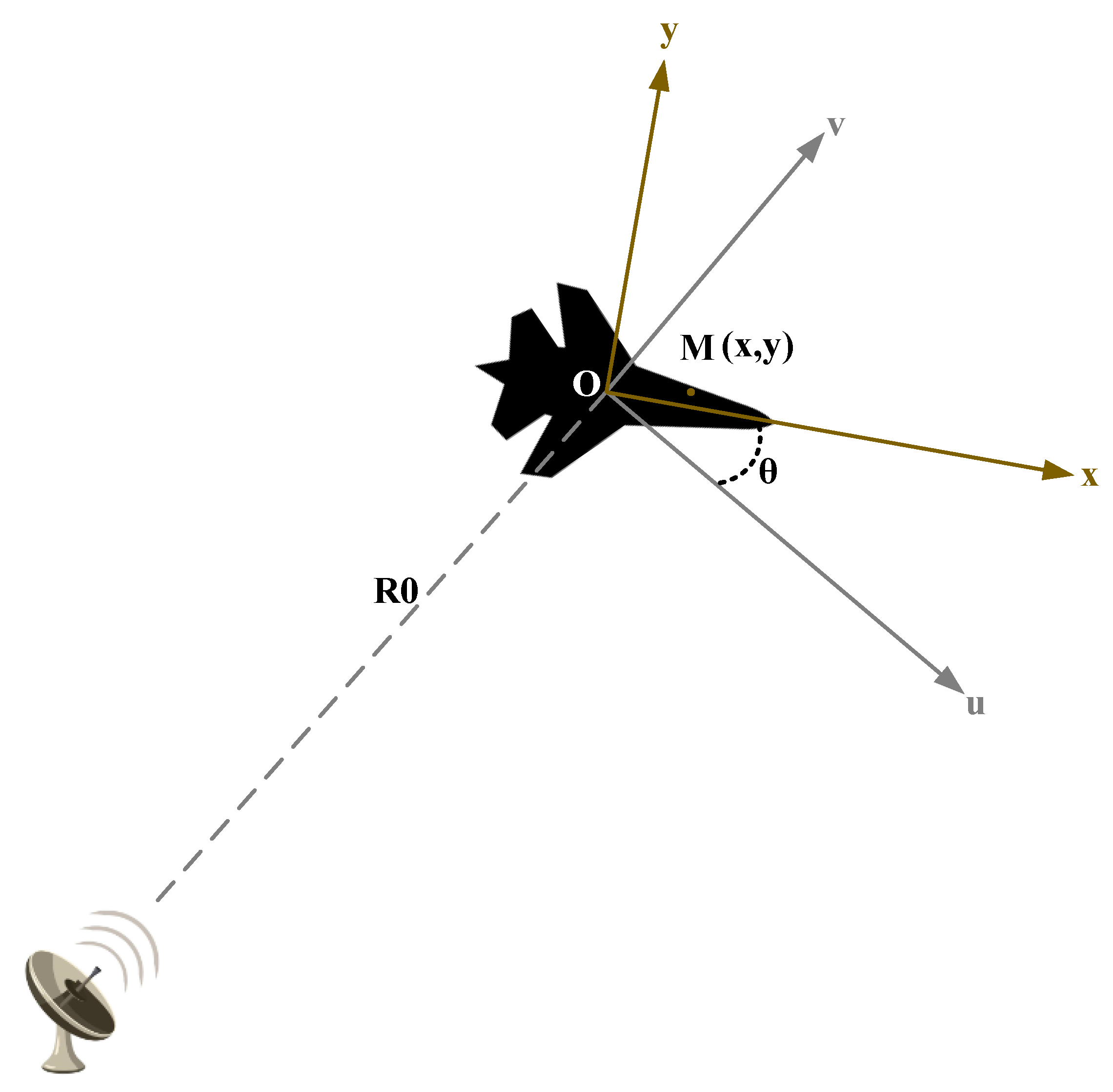
2.1. Two-Dimensional (2D) ISAR Imaging Turntable Model

In ISAR imaging, the motion of the target relative to the radar can be broken down into two components: the rotation of the target around its reference point and the translation of the target relative to the reference point [52]. Following motion compensation, only the rotational aspect is considered, and the target’s motion can be represented using a turntable model, as illustrated in Figure 1 [53]. This paper assumes far-field imaging conditions and that the translational component of the target has already been compensated for.

In Figure 1, the radar remains relatively stationary and is employed for target observation, while the aircraft, serving as the observed target, undergoes relative rotation. $uOv$ is the radar coordinate system that remains stationary relative to the radar; $xOy$ is the target coordinate system that remains stationary relative to the aircraft. $O$ is the center of rotation of the target, around which the target undergoes rotational motion. $R0$ represents the distance from the target center reference point to the radar. The observation angle $\theta$ represents the angle between the target coordinate system and the radar coordinate system. Its variation indicates the magnitude of the relative rotational angle between the target and the radar.

Assuming that ${\theta }_0$ is the initial angle between the target coordinate system and the radar coordinate system, $w_{\theta }$ and ${\alpha }_{\theta }$, respectively, represent the initial speed and acceleration of the target’s rotation, and $t_m$ represents the slow time, then

$$\theta ={\theta }_0+w_{\theta }{t}_m+\frac{1}{2}{\alpha }_{\theta }{t}_m^2$$

(1)

The correspondence between the $u-v$ coordinate system and the $x-y$ coordinate system is:

$$\mathrm{u}=x\cos \theta -y\sin \theta$$

(2)

$$v=x\sin \theta +y\cos \theta$$

(3)

Assuming that the coordinate of the $i$-th scattering point on the target in the target’s coordinate system is represented as $(x,y)$, the instantaneous distance between the point and the radar is:

$$\begin{array}{l}{R}_i=\sqrt{{(R0+v)}^2+u^2}\\ =\sqrt{R{0}^2+v^2+u^2+2R0\cdot v}\\ =\sqrt{R{0}^2+x^2+y^2+2R0\cdot v}\\ =\sqrt{R{0}^2+x^2+y^2+2R0(x\sin \theta +y\cos \theta )}\end{array}$$

(4)

When the distance is significantly greater than the size of the target, the above equation can be simplified as follows:

$$R_i\approx R0+x\sin \theta +y\cos \theta$$

(5)

${\tau }_i(s)$ is the round-trip delay between the $i$-th scattering point on the target and the radar,

$${\tau }_i(s)=\frac{2\times R_i}{c}$$

(6)

where $c$ is the speed of light. The stepped-frequency signal emitted by the radar can be modeled as [54]:

$$x(t)=\frac{1}{M}{\displaystyle \sum _{m=1}^M\frac{1}{\sqrt{T_p}}rect(\frac{t-m{T}_r}{T_p})\exp (j\pi k{(t-m{T}_r)}^2)}\exp (j{w}_{m}t)$$

(7)

where $w_m=2\pi (f_0+(m-1)\Delta f)$, $f_0$ is the starting frequency of the stepped-frequency signal transmitted, $\Delta f$ is the increment of frequency, $T_r$ represents the pulse repetition interval (PRI), $T_1$ denotes the width of the sub-pulse, $k=\frac{\Delta f}{T_1}$ signifies the FM slope of the chirp sub-pulse, and $M$ is the number of frequency points.

Suppose $P$ is the number of equivalent scattering center points on the target, then the radar’s received echo can be expressed as:

$$x_r(t,s)={\displaystyle \sum _{i=1}^P{\delta }_i[\frac{1}{M}{\displaystyle \sum _{m=1}^M\frac{1}{\sqrt{T_p}}rect(\frac{t-m{T}_r-{\tau }_i(s)}{T_p})\exp (j\pi k{(t-m{T}_r-{\tau }_i(s))}^2)}\exp [j{w}_m(t-{\tau }_i(s))]]}$$

(8)

where ${\delta }_i$ represents the target-scattering coefficient.

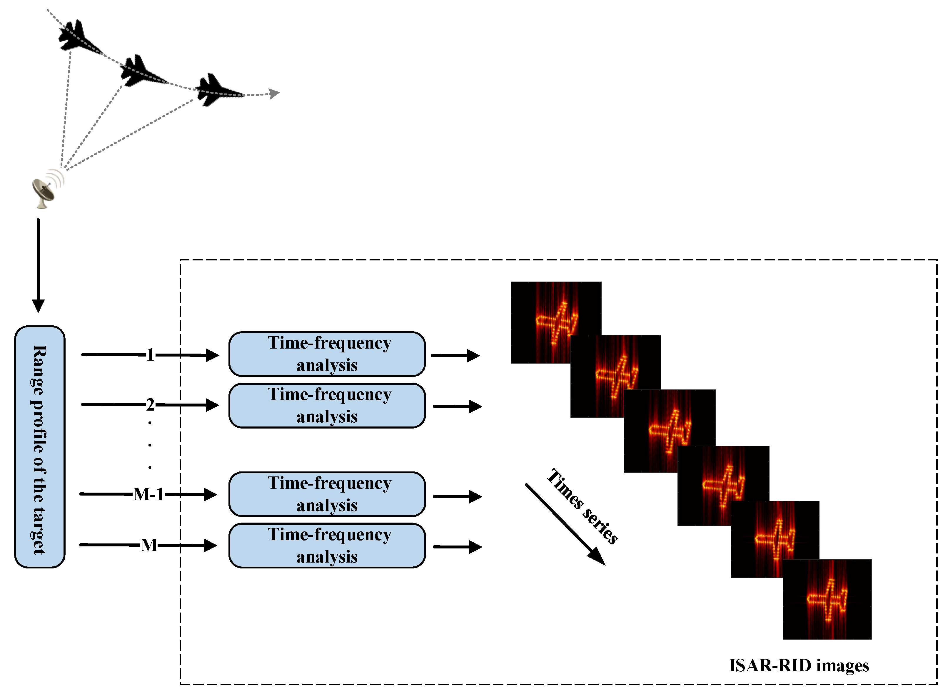
2.2. RID Imaging Theorem

Figure 2 illustrates the flow of the RID imaging algorithm. As shown in Figure 2, the RID algorithm exhibits similarities with the RDA when handling data in the range dimension. Both algorithms initially compress the echo data in the range dimension to generate a one-dimensional range profile. Afterwards, motion compensation is applied to the echo data based on the envelope and phase of the one-dimensional (1D) range profile. The crucial difference is that the RID algorithm uses TFA instead of FT employed in the RDA when the data is processed in the azimuth dimension. Consequently, the RID algorithm can obtain the Doppler transient value at any given time.

The STFT is a commonly used method for TFA. It operates by employing a sliding window mechanism where the size of the window and the step’s size can be adjusted. The window slides along the time-domain signal $x(t)$, and the FT is computed for each window. This process generates frequency-domain signals corresponding to different time windows. These signals are then combined to form a presentation of frequency changing over time, which is known as the time-frequency signal. The formula for the STFT is as follows:

$$STFT(t,w)={\displaystyle \int \mathrm{x}(\tau )}w(\tau -t)\exp (-jw\tau )d\tau$$

(9)

where $x(t)$ is the signal that needs to be processed, $w(t)$ represents a short-time wide window function, and $w(t)$ moves along the time axis with the change of time. Therefore, the frequency of the signal over time can be observed.

3. Method of ISAR Image Enhancement Using Neural Networks

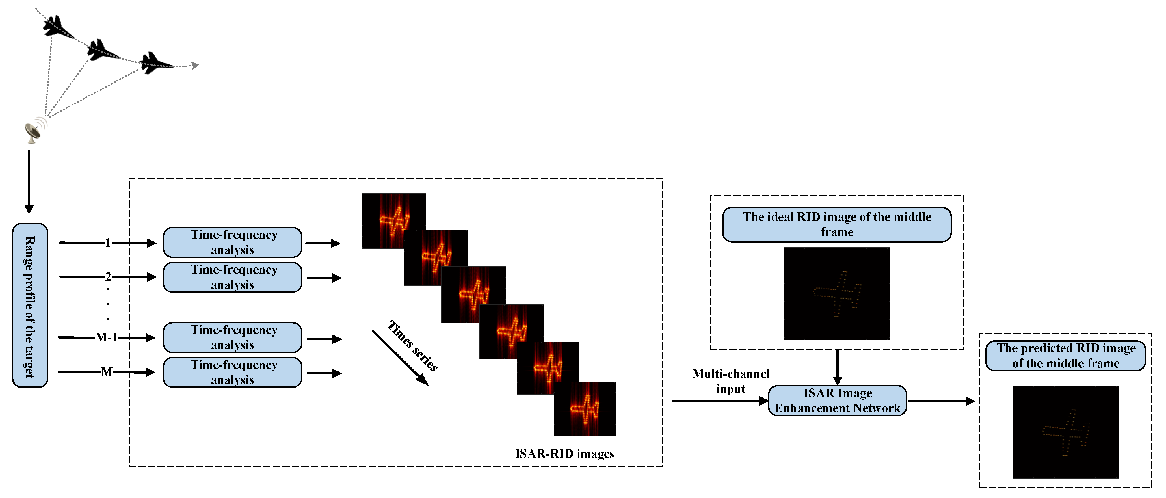
3.1. Flow of RID Image Enhancement

As the accumulated observation angle increases, the azimuthal resolution of ISAR images improves. However, a challenge arises when the angle increases beyond a certain threshold. The scattering points of the target undergo a phenomenon called “migration through range cells” (MTRC), leading to the shifting of one scattering point to the position of other scattering points. This phenomenon negatively affects the imaging process. Consequently, the image may not only be distorted but also potentially suffer from severe defocusing. As a result, the classical ISAR imaging algorithm, such as the RDA, may become invalid.

In this paper, our objective is to enhance the resolution of ISAR images while addressing azimuthal defocusing issues. We employ the RID imaging technique on the accumulated echo data that corresponds to defocused RDA images to achieve this. This enables us to capture multiple frames of RID images that encompass diverse scattering information of the targets. The consecutive RID images are input into the network for image enhancement, enabling the network to grasp and utilize the target characteristics effectively. To enhance the Doppler resolution in the RID images, we extend the duration of the time window as much as possible, while ensuring that the RID images remain focused. Finally, three consecutive ISAR-RID images are simultaneously input into the network to enhance the image of the intermediate frame. Through this approach, our objective is to address the issue of RDA imaging defocusing while improving the resolution of the ISAR image and reducing sidelobes.

Figure 3 illustrates the process of enhancing RID images using a neural network. Initially, the RID algorithm is applied to process the ISAR echoes and obtain RID images. Subsequently, the real and imaginary components of three consecutive RID images are input into the neural network as six channels. By training the network with the ideal RID image of the intermediate frame as the label, the network can learn the optimal mapping between inputs and outputs, ultimately generating high-resolution ISAR images. In practical applications, when we have approximate knowledge of the target’s distance range and radar parameters, it is unnecessary to possess specific information about the target’s characteristics. We can train a neural network by simulating point targets within the corresponding distance range. In such cases, it is possible to simulate ideal RID images.

3.2. Multi-Frame RID Network Structure

Figure 4 illustrates the network employed for enhancing the RID image. The network can be divided into six layers and three parts. The initial segment is the feature-extraction layer, encompassing the first convolutional layer. Its primary role is to extract features from radar images. The subsequent segment is the non-linear transformation layer, comprising convolutional layers two to five. These layers process the features extracted by the feature-extraction layer and convey them to the output layer. The final component is the output layer, consisting of the sixth convolutional layer, responsible for amalgamating the output data from the non-linear layers to form the enhanced ISAR image. Detailed information about the network structure’s parameters is provided in

Table 1. The parameters of the network’s structure.

Layer	Number of Channels	Kernel Size	Number of Kernels
Conv_1_ReLU	10	9 × 9	60
Conv_2_ReLU	64	3 × 3	124
Conv_3_ReLU	128	3 × 3	252
Conv_4_ReLU	256	3 × 3	124
Conv_5_ReLU	128	3 × 3	60
Conv_6	64	5 × 5	1

. After the first five convolutional layers, the ReLU activation function is used to help the network learn the nonlinear relationship between input and output, and its calculation speed is very fast. We use the ‘same’ convolution mode to ensure that the input and output image sizes remain the same. In addition, we configure the following training parameters: 200 epochs, a learning rate of 1 × 10⁻⁵, a batch size of four, weight decay of 1 × 10⁻⁵, and the Adam optimization algorithm.

Considering the different characteristics between the central and peripheral regions of the ISAR image, this paper introduces a positional encoding scheme for the ISAR image. This encoding serves to delineate the pixel positions within the ISAR image and comprises four channels. The relationship between the real and imaginary components of the ISAR image contains high-order information. When the complex ISAR image is directly fed into the neural network, it struggles to capture the image’s features effectively. Therefore, in this paper, the real and imaginary parts of the three ISAR-RID images are input into the network separately, resulting in a total of six channels for the image component. Consequently, the total number of input channels for the network is 10, including the real and imaginary parts of the three consecutive RID images received by the network and four channels for position encoding. The position encoding is also concatenated in the channel dimension after each convolutional layer.

For ISAR images, the defocusing level becomes more pronounced as the distance from the center of the scene increases. Additionally, defocusing in the azimuthal direction is more pronounced than in the range direction. In other words, the degree of defocusing varies between the horizontal and vertical directions of ISAR images. To address this characteristic, we designed a positional encoding scheme to indicate the pixel point locations within ISAR images. This allows the neural network to enhance its feature-learning capabilities when processing ISAR images. This encoding comprises radius encoding and angle encoding.

Figure 5 illustrates the layout of radius encoding and angle encoding. The encodings in Figure 5 serve as an example corresponding to a $10\times 10$ ISAR image. Figure 5a represents the radius encoding. As the distance from the image center increases, the color corresponding to the squares gradually transitions from green to lighter shades and then gradually changes to red. This indicates that further away from the ISAR image center, the level of defocus increases. In this representation, each square corresponds to a pixel point in the ISAR image, and the numerical value within each square represents the distance from the square’s center to the entire image’s center. In other words, it denotes the distance between the corresponding pixel point and the image center, essentially serving as a radius marker for that pixel. Additionally, complementary radius encoding is necessary to prevent the network from interpreting the radius encoding as weights during training instead of labeling. Therefore, the numerical value for each square in the complementary radius encoding is the complement of the corresponding square in the radius encoding. In other words, their values add up to the radius of the largest circle in the image.

Figure 5b depicts the angle encoding. Similarly, the color of each square changes based on the variation in the angle between the line connecting it to the image center and the x-axis. The value on each square represents its corresponding angle, specifically, the angle between the line connecting the element at the same position in the ISAR image as the square to the center point and the x-axis. Complementary angle encoding is necessary to ensure the network does not interpret these values as training weights. The sum of values at corresponding positions in complementary angle encoding and angle encoding is equal to $2\pi$.

3.3. Generation of Sample-Label Pairs

We selected a stepped-frequency signal with a frequency range of 8.8 to 9.2 GHz, with a step size of 5 MHz, totaling 80 steps for our simulated experiments. In this paper, the direction of range refers to the axis parallel to the direction of radar propagation toward the target, and the azimuth direction is defined as the axis perpendicular to the direction of range. The overall range for the scene’s range direction is from −20 to 20 m, and the azimuth range is also from −20 to 20 m. We divide the imaging scene into 400 grids in the range direction and 500 grids in the azimuth direction. As a result, the grid size of each range element is 0.1 m, and the grid size of each azimuth element is 0.08 m.

The actual imaging scene of the point targets in this paper spans the range direction of (−8, 8) meters and the azimuth range of (−6, 6) meters. Within this scene, we randomly generate a maximum of 200 point targets, which rotate at a uniform speed. In this paper, we define a specific observation angle range of six degrees for each RID image frame, with 3-degree rotation occurring between adjacent frames. To maintain the focus of the RID image while maintaining the highest possible resolution, we set the RID image to just avoid defocusing. This ensures that the RID image maintains focusing and the highest possible resolution. We found through experiments that this condition can be met when the target rotation speed is 37.497°/s, which means the target rotates at an angle of 37.497° per second, the STFT window length is 158, and the noverlap is 79. Each set of sample-label pairs includes three consecutive RID images and the ideal RID image of the intermediate frame. The ideal coordinates of the targets in the RID image are convolved with a Gaussian kernel function to obtain the ideal RID image, which serves as the label. Its expression is as follows:

$$I(x,y)={\displaystyle \int {\displaystyle \int T(u,v)\cdot h(x-u,y-v)dudv}}$$

(10)

where $T(u,v)$ is the function of the target, $I(x,y)$ denotes the synthesized reconstructed image of the target, and $h(x,y)$ is the PSF of the ISAR imaging system. It should be noted that in this paper, the Gaussian kernel function is chosen as the point-spread function (PSF) because it reduces the sidelobes of the label image compared to the sinc function [40].

A total of 3000 sets of sample-label pairs are generated as the training set and 1000 sets as the validation set. The images in the dataset have a size of 256 × 256. Figure 6 shows the coordinate plot of the point targets in the imaging scene, the low-resolution RID image of the intermediate frame, and its corresponding ideal image.

The resolution of ISAR is defined as the width of the half-power point in the target impact response, that is, the width of the 3 dB main lobe. This resolution measurement indicates the minimum distance that ISAR can distinguish between two adjacent scattering points on the target.

Cross-range resolution is determined by the wavelength of the radar’s emitted signal and the target’s rotation angle relative to the radar. The actual cross-range resolution is calculated using the formula:

$${\rho }_a=\frac{\lambda }{2\Delta \theta }$$

(11)

where $\lambda$ is the signal’s wavelength and $\Delta \theta$ is the rotation angle of the target relative to the radar during the imaging time.

In this paper, the simulated point targets have a total rotation angle of 19.44° and a wavelength of 0.0333 m, so the cross-range resolution is about 0.049 m.

The range resolution of the radar is determined by its bandwidth, and the formula is:

$${\rho }_{\mathrm{r}}=\frac{c}{2B}$$

(12)

where $B$ is the bandwidth of the signal transmitted by the radar. From this section, it can be known that the simulated step size of the stepped-frequency signal is 5 MHz, with a total of 80 steps. Consequently, its bandwidth is 0.4 GHz, leading to a determined range resolution of 0.375 m.

3.4. Design of Non-Equilibrium Loss Function

The loss function plays a pivotal role in machine learning as it quantifies the disparity between predicted and ground-truth values. A lower loss value signifies greater precision in the model’s predictions. In deep learning-based radar imaging methods, an end-to-end training system is employed to minimize the loss function’s value between predicted images and ground truth, aiming for accurate predictions.

However, the imbalance between the number of pixels occupied by the target and the number of pixels in the non-target region can lead the network to have a greater inclination towards regressing to the non-target region, rather than focusing on the target itself during the training process. The existing loss functions cannot optimize the network parameters effectively for the specific characteristics of ISAR images, thus hindering the attainment of improved training results. Therefore, it is imperative to design suitable loss functions tailored to ISAR images, which can aid the network in learning the relevant features, facilitating faster convergence and leading to more accurate predictions.

A similar imbalance exists in the field of object detection. To address the issue of categories’ imbalance in the field of object detection, Focal Loss is proposed in [55] on the basis of the cross-entropy loss function, aiming to adjust the proportion of positive and negative samples. The calculation of the cross-entropy loss function is as follows:

$$Cros{s}_{-}Entrop{y}_{-}Loss=\left\{\begin{array}{c}lo{g}_{2}p,y=1\\ \mathrm{l}o{g}_2(1-p),y=0\end{array}\right.$$

(13)

The formula of Focal Loss is as follows:

$$Foca{l}_{-}Loss=\left\{\begin{array}{c}-\alpha {(1-p)}^{\gamma }{\log }_{2}p,y=1\\ -(1-\alpha )p^{\gamma }{\log }_2(1-p),y=0\end{array}\right.$$

(14)

where $\alpha$ is the balancing factor for adjusting the proportion of positive and negative samples, $y$ denotes the truth class, and $p\in [0,1]$ represents the model’s estimated probability for the class $y=1$. $\gamma$ is used to control the rate of reduction in sample weight. When $\gamma$ is set to 0, the Focal Loss function degenerates into the cross-entropy loss function, and when $\gamma$ increases, the impact of the adjustment factor becomes more pronounced.

In the field of image regression, MSE is the most commonly used loss function, and its formula is:

$$MSE(p,y)=\frac{{\displaystyle \sum _{i=0}^m{(p^{(i)}-y^{(i)})}^2}}{m}$$

(15)

where $p^{(i)}$ represents the predicted value, $y^{(i)}$ is the ground-truth value, and $m$ is the total number of pixels. However, the MSE loss function uniformly weights all pixel points in the image. Thus, as mentioned above, it cannot resolve the imbalance issue encountered in ISAR images.

This paper proposes a solution by combining the Focal Loss’s concept with the MSE loss function. We first normalize the values of the label’s pixels and then weight the loss function based on these normalized values. Higher weights are assigned to pixels corresponding to the target, while lower weights are given to pixels at non-target locations. This approach enables the network to prioritize accurate reconstruction of the target’s region during training.

The formula for the improved loss function is as follows:

$$IMSE(p,y)=\frac{1}{\mathrm{m}}{\displaystyle \sum _{i=1}^m[{(p^{(i)}-y^{(i)})}^2(1+\frac{y^{(i)}}{{\displaystyle \sum _{j=1}^m{y}^{(j)}}})]}$$

(16)

3.5. Evaluation Indices

3.5.1. Mean Squared Error (MSE)

MSE calculates the average squared difference between the values of pixels in the ideal image and the predicted image. This operation allows us to measure the disparity between the two images and is the primary method for objectively assessing image quality. The following formula gives it:

$$MSE=\frac{1}{\mathrm{m}\times n}{\displaystyle \sum _{i=0}^m{\displaystyle \sum _{j=0}^n\left|\right|P(i,j)-I(i,j)|{|}^2}}$$

(17)

where $I$ denotes the ideal radar image of size $m\times n$ and $P$ represents the image predicted by the network. $m$ and $n$ represent the number of pixel points in the horizontal and vertical directions of the image, respectively. A smaller MSE value indicates a better regression effect of the network on the image.

3.5.2. Peak Signal-to-Noise Ratio (PSNR)

PSNR is a ratio of the maximum pixel value to the intensity of noise, primarily used to gauge the algorithm’s noise-removal capability. A higher PSNR value indicates the superior noise-suppression performance of the algorithm [56]. The formula for PSNR is as follows:

$$\begin{array}{l}PSNR=10lo{g}_{10}(\frac{\max {(I)}^2}{MSE})\\ =10lo{g}_{10}(\frac{\max {(I)}^2}{\frac{1}{m\times n}{\displaystyle \sum _{i=0}^m{\displaystyle \sum _{j=0}^n\left|\right|P(i,j)-I(i,j)|{|}^2}}})\end{array}$$

(18)

3.5.3. Image Entropy

For an ISAR image with a size of $M\times N$, its image entropy can be defined as:

$$H=-{\displaystyle \sum _{m=1}^M{\displaystyle \sum _{n=1}^N{P}_{mn}\ln P_{mn}}}$$

(19)

where

$$P_{mn}=\frac{K(m,n)}{{\displaystyle \sum _{m=1}^M{\displaystyle \sum _{n=1}^{N}K(m,n)}}}$$

(20)

where $K(m,n)$ represents the value of the pixel at position $(m,n)$ in the image, and $P_{mn}$ represents the probability of $K(m,n)$ in the image. The lower the entropy of an ISAR image, the more information it contains, indicating better focusing performance. Conversely, if the image has poor focus, it will have higher entropy and appear less clear.

3.5.4. Contrast

Contrast reflects the variation in pixel intensity in an image. A higher contrast indicates a more pronounced distinction in intensity, suggesting a greater probability of the presence of strong scattering points. Conversely, a lower contrast suggests a lower likelihood of the presence of strong scattering points. Its definition is as follows:

$$C=\frac{\sqrt{E\left\{{[K^2(m,n)-E\{K^2(m,n)\}]}^2\right\}}}{E\{K^2(m,n)\}}$$

(21)

4. Experimental Results

4.1. Predicted Results of Point Targets

The trained network is initially validated using point targets described in Section 3.3. Figure 7a–c depict low-resolution point targets’ RID images of three consecutive frames, respectively. Figure 7d displays the ideal image of the intermediate frame, while Figure 7e shows the predicted result obtained from a network trained using the method proposed in this paper.

Figure 7 shows that the predicted results of the proposed method closely resemble the ideal image. Subsequently, the aircraft scattering-point model, comprising 68 point targets, was employed to further validate the effectiveness of the proposed method. In addition to comparing the IMSE loss function proposed in this paper with the traditional MSE loss function, we also conducted a comparative experiment using the method described in [50]. This method employs an improved U-Net network for the super-resolution processing of defocused ISAR images. Since it tackles the same problem we aim to address in this paper, namely defocusing in wide-angle ISAR imaging, we chose to utilize this method for a comparative experiment.

Figure 8a–c illustrate the relative rotation of RID images across different frames, with these images possessing relatively low resolution. Figure 8d depicts the defocused RDA result. Figure 8f illustrates the remarkable enhancement effect of U-Net on the target points, where pixel values even exceed those in the ideal RID image. Nevertheless, the image suffers from an excessive amount of clutter interference. Figure 8g,h demonstrate that a network trained with IMSE produces a prediction with higher resolution compared to the one obtained using the MSE loss function. Especially at the three green markers, it can be seen that the point targets in Figure 8h has fewer sidelobes and are closer to the ideal image.

Since the comparison between Figure 8g,h is not particularly pronounced, to better validate the superiority of the loss function proposed in this paper, we list the evaluation metrics values for the images predicted by three methods in

Table 2. Evaluation metrics of the predicted images obtained by different methods.

Loss Function	MSE	PSNR	Entropy	Contrast	Runtime
MSE	0.0035	24.3612	36.5252	3.7185	0.4738
IMSE (proposed)	0.0019	27.1167	25.3929	6.7649	0.4799
U-Net	0.0049	23.0684	11.5343	11.4111	0.1940

. Since we normalized the image matrices before computing the MSE evaluation metric, the calculated results are relatively small, and the differences between the results are also relatively minor. Furthermore, since PSNR is computed based on MSE, the variations in PSNR are also relatively small.

Clearly, compared to the MSE loss function, the proposed IMSE outperforms in the first four evaluation metrics, indicating its better suitability for the ISAR image-enhancement task. However, it comes with the trade-off of a relatively longer computation time. Nevertheless, the U-Net’s predicted image exhibits the best performance among the three methods in terms of the evaluation metrics: entropy, contrast, and runtime.

4.2. Input Data Settings

The positional encoding and the number of input RID images are critical parameters within our input samples. To validate the effectiveness of the proposed positional encoding, we utilized MSE as the loss function and separately trained the network illustrated in Figure 4, alongside its corresponding network that lacks positional encoding. As depicted in Figure 9, the network with positional encoding converges more rapidly during the training process. Furthermore, after the network training stabilizes, its training loss values are lower, indicating that its predicted images are closer to the ideal images. The validation losses also confirm this point, suggesting that it still holds on untrained datasets and has a good generalization ability. This indicates that the proposed positional encoding is beneficial for our task.

Subsequently, to validate the effectiveness of the proposed three-frame input method, we conducted experiments utilizing the single-frame, three-frame, and five-frame input methods, respectively. In Figure 10a, these three methods demonstrate a comparable convergence rate throughout the network-training process. As the network training stabilizes, the three-frame input method exhibits a slightly lower training loss than the other two methods. In comparison, the loss value of the single-frame input method is slightly higher. In Figure 10b, the five-frame input method converges first, but its curve stabilizes with the highest loss value. The convergence speed of the single-frame and three-frame input methods is similar. After the curve stabilizes, the loss value of the three-frame input method is lower. This indicates that the three-frame input method performs well on both the training and validation sets and is suitable for this paper’s ISAR image-regression task.

We observe an insignificant disparity in loss values between the three-frame input method and the single-frame input method. As mentioned, the loss values are computed after normalizing the image matrix. This leads to a relatively small numerical value for the MSE and a relatively small difference in loss values between different methods.

4.3. Robustness Verification against Noise

To evaluate the robustness of the proposed method against noise, we introduced noise into the test data. It is important to emphasize that the training data remained pristine, without any artificially added noise, throughout the experiments conducted in this paper.

In research, the amplitude-probability distribution model and clutter correlation spectrum are commonly used to characterize clutter. However, solely studying the single-point amplitude characteristics of clutter is generally insufficient, and it is crucial also to consider the correlation properties between pulses. The correlation between clutter-echo signals is generally described by correlation models, including time-correlated models and spatially correlated models.

The temporal correlation of clutter is commonly depicted through the clutter power spectrum, representing the correlation among clutter echo signals originating from the same region. In other words, it signifies the correlation between various echo pulses within the same clutter-distance resolution unit. This concept is typically encompassed by models such as the Gaussian spectral model, the Cauchy spectral model, and the Allpole spectral model, among others. However, there have been relatively few studies focusing on spatial correlation. In many studies, the spectrum of radar clutter is represented by a Gaussian spectrum [40,41,43,47]:

$$S(f)=\exp (\frac{-{(f-f_{\mathrm{d}})}^2}{2{\sigma }_f{}^2})$$

(22)

where ${\sigma }_f$ represents the standard deviation of the clutter’s distribution (${\sigma }_f=\frac{2{\sigma }_v}{\lambda }$, ${\sigma }_v$ is the root mean square of the clutter velocity, and $\lambda$ is the wavelength of the radar), and $f_{\mathrm{d}}$ represents the average Doppler frequency of the clutter.

Given that the Gaussian spectrum characterizes noise in the frequency domain, we incorporate Gaussian noise with SNRs of −10 dB, −20 dB, −30 dB, and −40 dB the one-dimensional range profile separately. The results obtained by RDA, RID, and the proposed method under different SNR conditions are shown in Figure 11.

It is evident that, as the SNR decreases, image clutter becomes increasingly pronounced. Under conditions with SNRs of −10 dB and −20 dB, both RDA and RID images are significantly impacted by noise. Nevertheless, the neural network generates superior predictions. At an SNR of −30 dB, while there are numerous fake points in the predicted image, the outline of the aircraft remains clear and distinguishable. However, as the SNR drops further to −40 dB, the clutter in the prediction becomes more pronounced, ultimately obscuring the aircraft’s contour. This indicates that the proposed method has a certain degree of robustness against noise.

Table 3. MSE and PSNR of the predicted result under different SNRs.

SNR (dB)	MSE	PSNR (dB)
No noise	0.0019	27.1167
−10	0.0019	27.1167
−20	0.0022	26.5856
−30	0.0025	26.1045
−40	0.0032	24.9574

presents the MSE and PSNR values obtained through the proposed method at various SNRs. The data in the table consistently demonstrates a gradual increase in MSE and a decrease in PSNR as the SNR decreases. This observation aligns with the trends depicted in Figure 11. This further substantiates the method’s ability to exhibit a certain degree of robustness in the presence of noise.

4.4. Predicted Results of Full-Wave Simulated Data

In this section, we perform experiments using full-wave data simulated with FEKO (https://www.tiaozhanbei.net/, accessed on 19 October 2023) [57], provided by the Laboratory of Pinghu, to evaluate the effectiveness of the proposed method. Furthermore, considering the challenge associated with incomplete signals encountered in practical ISAR target imaging, we randomly down-sample the echo data of the training samples to obtain incomplete signals. Subsequently, we perform validation experiments to assess the robustness of the proposed method against incomplete signals.

4.4.1. Full Data Validation

The experimental results are depicted in Figure 12 and Figure 13. Consistent with the training samples, in this experiment, the observation angle corresponding to the RID image of each frame is set to 6 degrees, and the observation angles between adjacent frames are rotated by 3 degrees relative to one another.

Figure 12e is unable to fully reconstruct the target’s image. Compared to Figure 12b, both Figure 12f,g display a clearer target outline and higher resolution. Moreover, Figure 12g recovers more information of the target compared to Figure 12f. Nevertheless, it is worth noting that Figure 12g also contains slightly more noise in non-target areas than Figure 12f.

Figure 13e recovers fewer target details and displays noticeable interference around the target area compared to Figure 13f,g. Figure 13f, in contrast to Figure 13g, exhibits slight interference noise around the target.

4.4.2. Down-Sampled Data Validation

In this section, we down-sample the full-wave data at a down-sampling rate of 5% to train the network. Additionally, the full-wave data are down-sampled at rates of 10%, 20%, 30%, and 40%, respectively, to assess the robustness of the method proposed in this paper when dealing with incomplete data. Figure 14 presents the RID imaging results of the intermediate frame under various down-sampling conditions, the enhanced results achieved by the network trained on complete data, and the improved results obtained by the network trained on down-sampled data.

As the down-sampling rate increases, the imaging quality of RID deteriorates. It can be observed that the network trained with down-sampled data produces more explicit predictions with less noise compared to those obtained by the neural network trained with complete data. Particularly, when the down-sampling rate is set to 10%, the prediction from the network trained with down-sampled data exhibits extremely low noise levels and sharper target outlines.

5. Discussion

In this section, we conduct an in-depth discussion of the above experimental results.

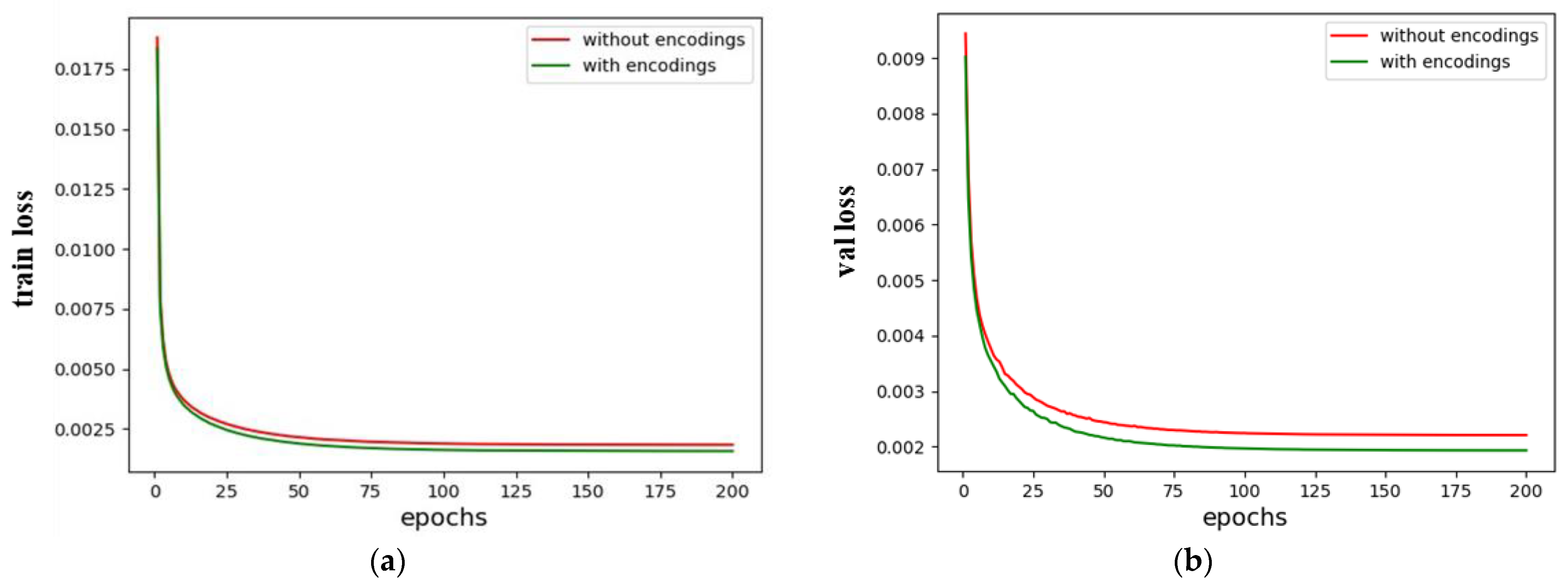
• The results shown in Figure 9 demonstrate the effectiveness of the positional encoding we proposed in our study. We independently train networks with and without positional encoding in Section 4.2, producing training and validation loss curves. During training, the network with positional encoding converges more quickly. The network displays lower loss values when its training stabilizes, and the validation set shows the same trend. This experimental finding suggests that positional encoding can be designed for the ISAR image-enhancement task in a way that effectively identifies the position of pixels based on the variable degrees of defocusing at various locations in ISAR images. This discovery significantly impacts our following study on the defocusing of ISAR;
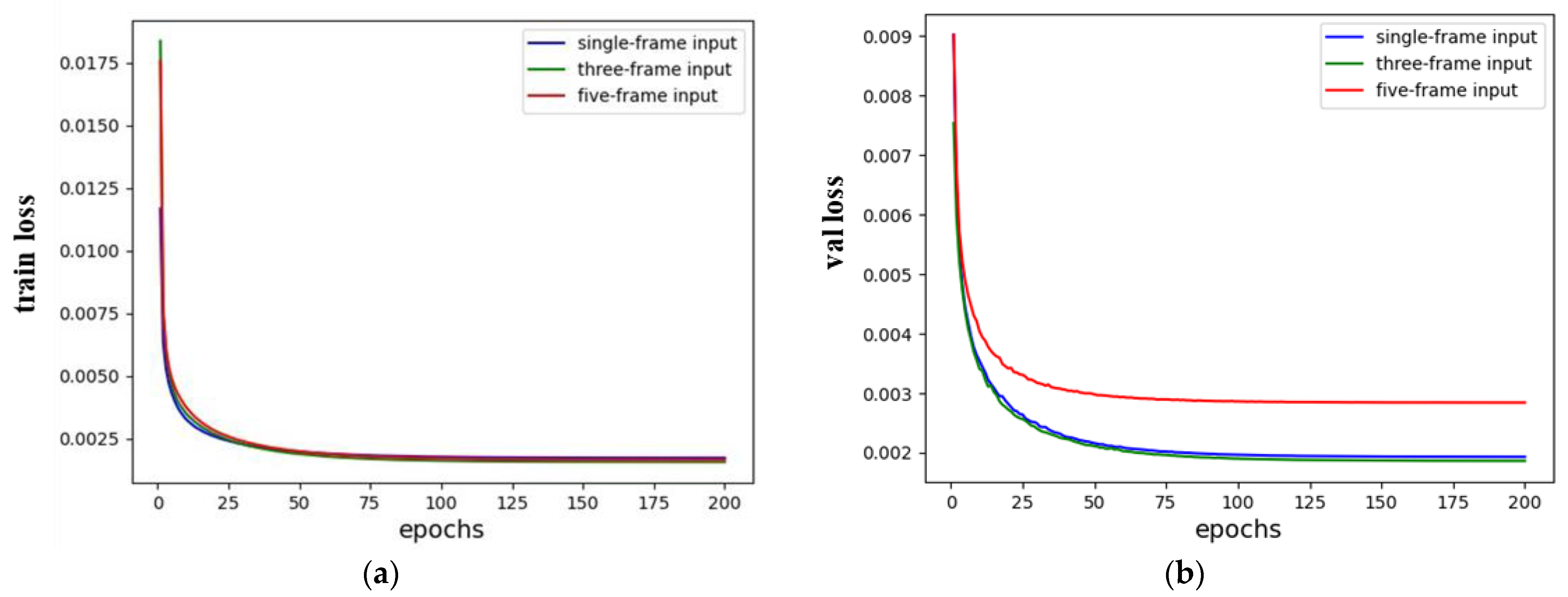
• Figure 10 demonstrates the benefits of using the three-frame input method suggested in this paper for our ISAR-RID image-enhancement task. This is explained by the fact that the multi-frame input approach, as opposed to the single-frame input method, gives the network more information about the target, allowing the network to understand the features of the target better. On the other hand, the five-frame input method introduces excessive redundant information relative to the three-frame input method, leading to the network’s inability to precisely learn the target’s features. Therefore, the three-frame input method is better suited to our task;
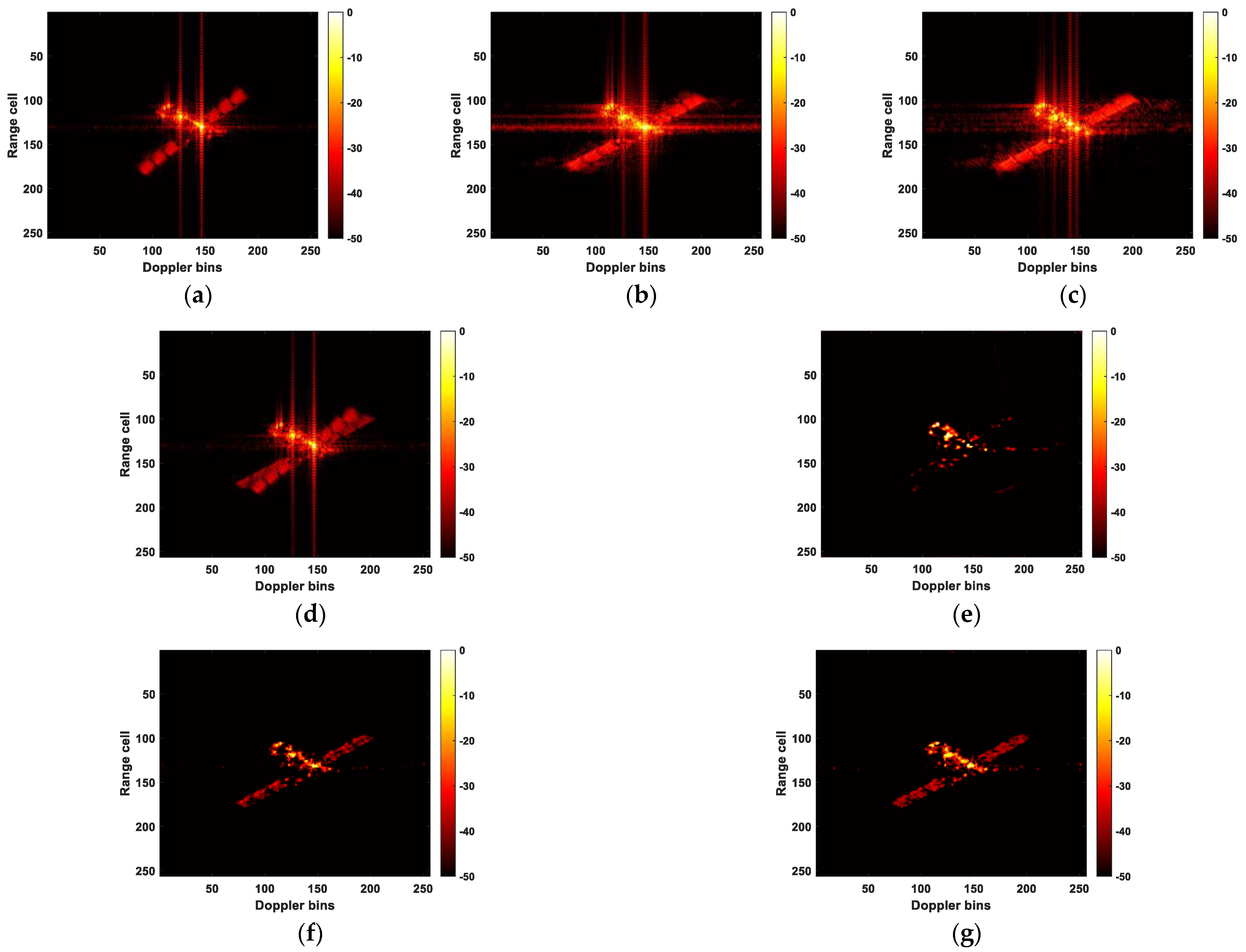
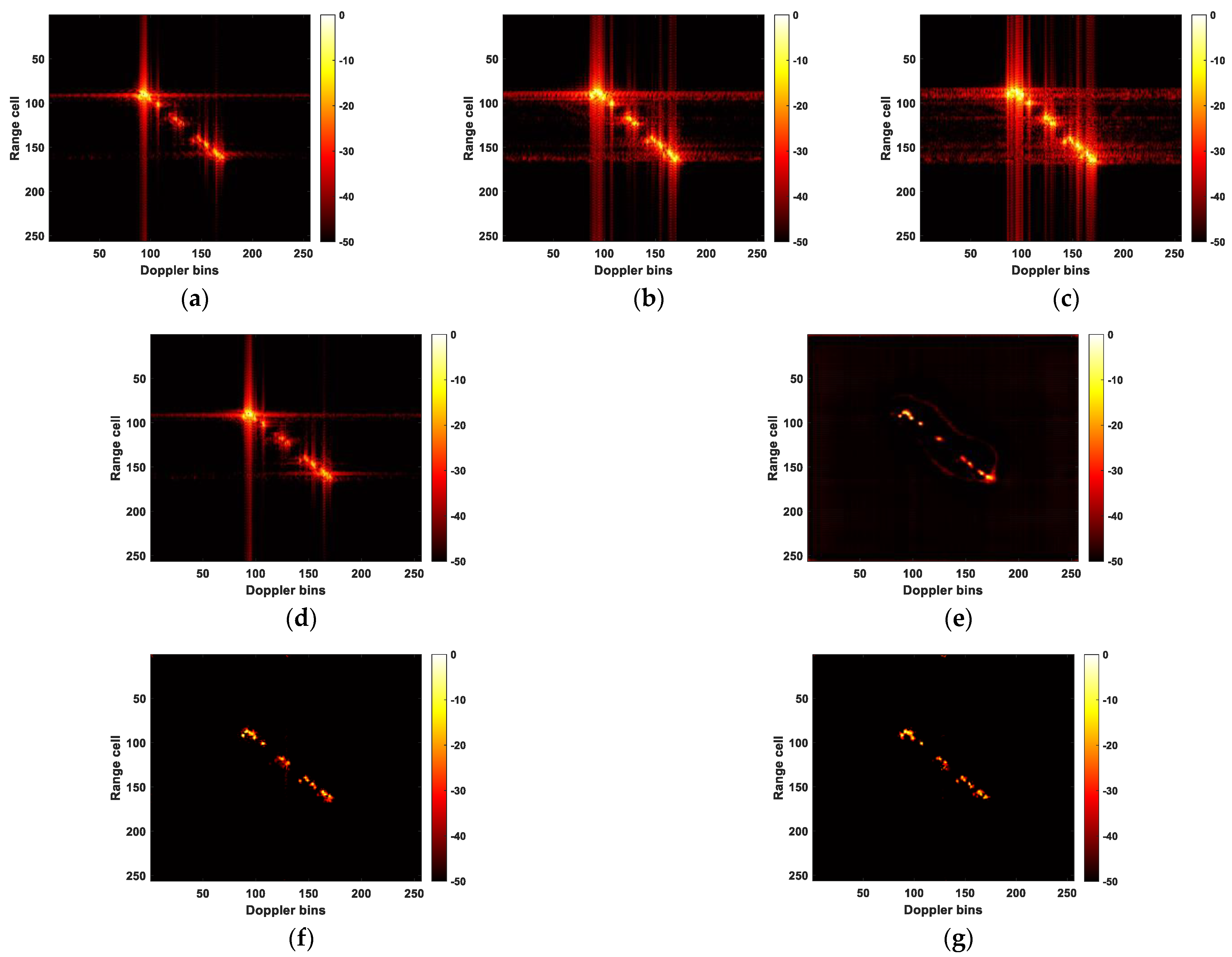
• The experimental results clearly show that the approach provided in this research works better than the one in [50]. Figure 8f exhibits significant noise interference and excessive enhancement of the target points, surpassing the pixel values in the ideal image. It is precisely because of the excessive enhancement of strong scattering points that U-NET performs the best in terms of entropy and contrast in Table 2. In Figure 12e, the target is incompletely recovered, while in Figure 13e, although the target is recovered, it lacks fine details. Moreover, noticeable noise interference is present around the target in Figure 13e. These three experiments collectively demonstrate that the proposed method, regardless of whether MSE or IMSE is used as the loss function during network training, achieves superior results in terms of target recovery and noise elimination compared to [50]. Thus, this also validates the effectiveness of the proposed three-frame RID image input method and position encoding. It is crucial to highlight that the U-Net exhibits the fastest runtime, more than twice as speedy as the other two methods. Furthermore, the MSE loss function is marginally quicker compared to the IMSE. This underscores that the proposed method comes at the expense of processing time, which is a challenge we must tackle in our future research endeavors;
• To address the characteristics of ISAR images, this paper proposes an improved loss function. By emphasizing the regression of pixel intensities within the target region during the training process, it overcomes the inherent limitations of the MSE loss function, which treats all pixels equally. This improvement ensures that the network focuses more effectively on the target itself rather than non-target areas. The resolution of the target in Figure 8h surpasses that in Figure 8g. Figure 12g recovers more target information compared to Figure 12f. There is slight clutter noise around the target in Figure 13f, resulting in a slightly inferior predictive performance compared to Figure 13g. These three experiments collectively highlight the significance of the proposed loss function in this paper, as it encourages the neural network to concentrate more on accurately estimating the target area within ISAR images. Certainly, as depicted in Table 2, the predictions produced by the proposed IMSE consistently outperform MSE in the initial four evaluation metrics: MSE, PSNR, Entropy, and Contrast. This further strengthens the evidence of its effectiveness as a loss function. However, it is worth noting that the use of IMSE does come with the trade-off of increased computational time. This is indeed a limitation of the method and is an issue that we need to address in our future work;
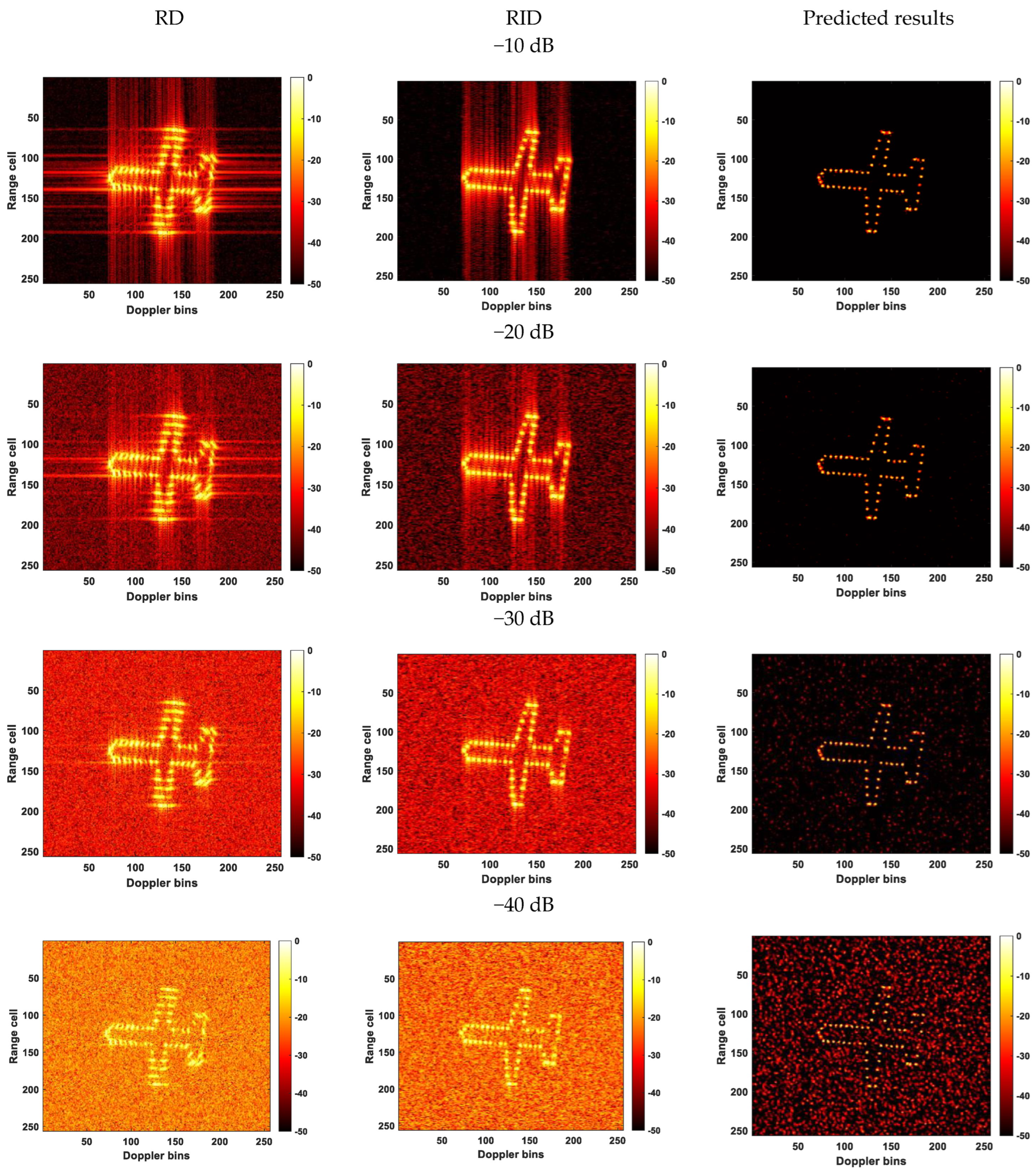
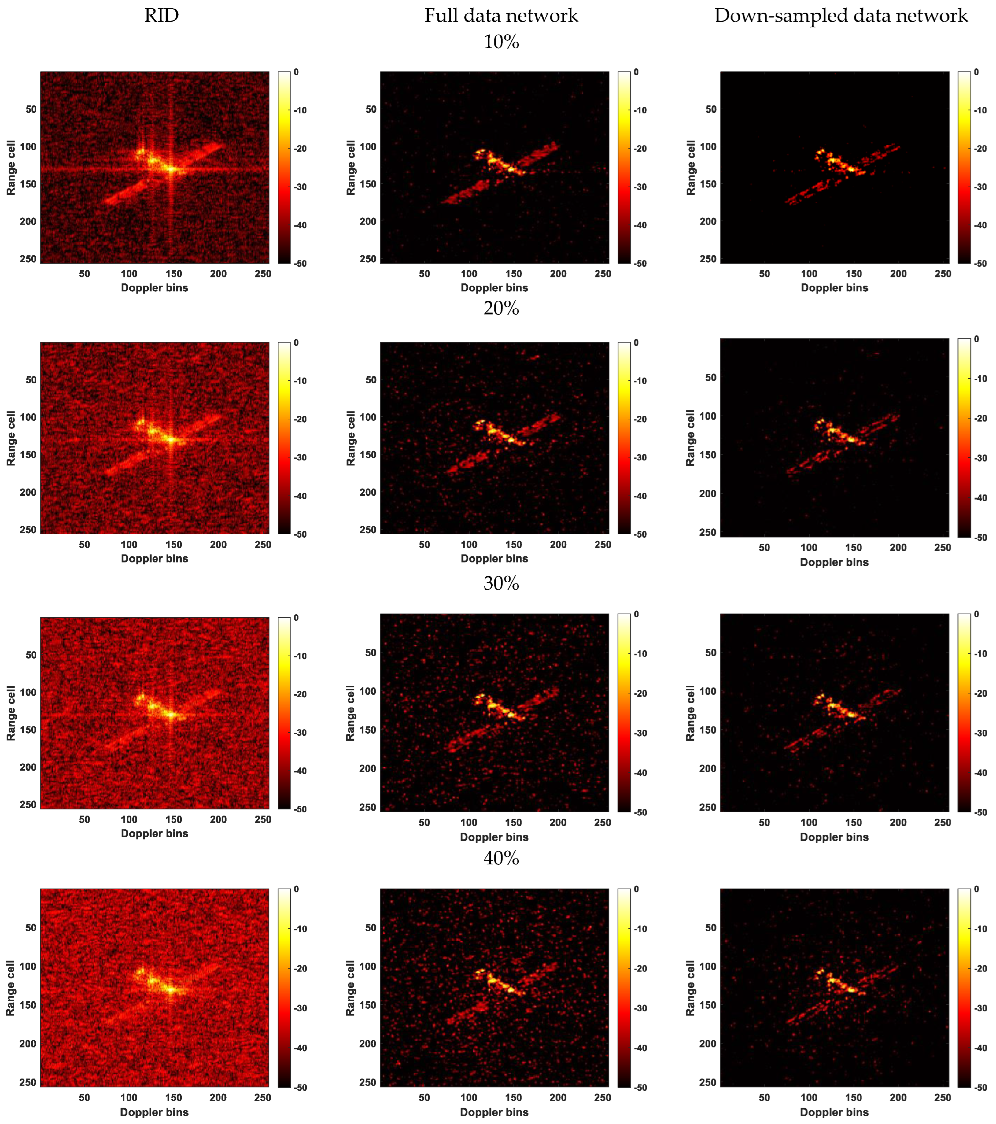
• The proposed method demonstrates a certain level of robustness to noise and incomplete data. As demonstrated in Figure 11 and Figure 14, within a certain range of noise and down-sampling conditions, the trained network is still capable of accurately predicting ISAR images. Specifically, in the robustness test against noise, our network is trained on samples without noise. However, it achieved accurate and high-resolution predictions at SNRs of −10 dB and −20 dB. Even at −30 dB, although the predicted image contains noise, the target’s contour is still clearly discernible. For the robustness experiment against incomplete data, we separately use the network trained on the full dataset and the network trained on the dataset down-sampled at 5% to predict data down-sampled at different rates. It can be observed that both networks exhibit a certain level of robustness. However, the network trained on the down-sampled data yields slightly better-predicted results. This finding suggests that using training data specific to different scenarios or imaging conditions can improve the network’s prediction performance and make it more practical.

6. Conclusions

This research presents an improved ISAR-RID imaging method based on deep learning to increase resolution while addressing the defocusing issues in wide-angle ISAR imaging. We introduce a multi-frame RID input method to allow the network to obtain more information about the targets. We propose positional encoding to denote pixel locations, since ISAR images exhibit differing degrees of defocusing at various positions. To tackle the challenge of imbalanced pixel counts between target and non-target areas in ISAR images, we have improved the loss function by incorporating Focal Loss. This modification focuses the network’s attention during training more on target regression. Experimental results demonstrate the effectiveness of our proposed approach in addressing defocusing issues and enhancing resolution in ISAR imaging under wide-angle conditions. In practical applications, when we know the approximate imaging distance and radar parameters, we can use this method to simulate point targets within the corresponding distance range for training the network. Subsequently, we can apply this trained network to actual observed targets.

Notwithstanding the efficacy of the suggested approach, we concede the existence of certain constraints. While the three-frame input method and position encoding enhance the network’s performance in ISAR image enhancement, they do so at the expense of increased processing time. Moreover, while IMSE improves the network’s capacity to focus on enhancing target regions, its effects are not very pronounced. Our experiments were conducted on uniformly rotating targets after motion compensation, whereas most real-world scenarios involve non-uniformly moving targets.

In future work, we plan to do away with the need to mosaic position encoding after each convolutional layer by directly integrating position encoding into the neural network design. To further improve the loss function’s performance, we also intend to refine it. Building upon these enhancements, we will explore solutions for the challenging task of enhancing large-angle imaging for non-uniformly moving targets, thus making our approach more suitable for practical applications. Summing up, despite certain limitations in our study, it provides a novel perspective for the future of ISAR large-angle imaging. Furthermore, it establishes a foundational basis for subsequent target detection and recognition.

References

1. Yang, S.; Li, S.; Jia, X.; Cai, Y.; Liu, Y. An Efficient Translational Motion Compensation Approach for ISAR Imaging of Rapidly Spinning Targets. Remote Sens. 2022, 14, 2208. [Google Scholar] [CrossRef]
2. Zhu, X.; Jiang, Y.; Liu, Z.; Chen, R.; Qi, X. A Novel ISAR Imaging Algorithm for Maneuvering Targets. IEEE Geosci. Remote Sens. Lett. 2022, 19, 1–5. [Google Scholar] [CrossRef]
3. Liu, F.; Huang, D.; Guo, X.; Feng, C. Unambiguous ISAR Imaging Method for Complex Maneuvering Group Targets. Remote Sens. 2022, 14, 2554. [Google Scholar] [CrossRef]
4. Yang, Z.; Li, D.; Tan, X.; Liu, H.; Liao, G. An Efficient ISAR Imaging Approach for Highly Maneuvering Targets Based on Subarray Averaging and Image Entropy. IEEE Trans. Geosci. Remote Sens. 2021, 60, 1–13. [Google Scholar] [CrossRef]
5. Huang, P.; Xia, X.G.; Zhan, M.; Liu, X.; Jiang, X. ISAR Imaging of a Maneuvering Target Based on Parameter Estimation of Multicomponent Cubic Phase Signals. IEEE Trans. Geosci. Remote Sens. 2021, 60, 1–18. [Google Scholar] [CrossRef]
6. Jiang, Y.; Sun, S.; Yuan, Y.; Yeo, T. Three-dimensional aircraft isar imaging based on shipborne radar. IEEE Trans. Aerosp. Electron. Syst. 2016, 52, 2504–2518. [Google Scholar] [CrossRef]
7. Yang, Z.; Li, D.; Tan, X.; Liu, H.; Liu, Y.; Liao, G. ISAR Imaging for Maneuvering Targets with Complex Motion Based on Generalized Radon-Fourier Transform and Gradient-Based Descent under Low SNR. Remote Sens. 2021, 13, 2198. [Google Scholar] [CrossRef]
8. Wang, T.; Wang, X.; Chang, Y.; Liu, J.; Xiao, S. Estimation of Precession Parameters and Generation of ISAR Images of Ballistic Missile Targets. IEEE Trans. Aerosp. Electron. Syst. 2010, 46, 1983–1995. [Google Scholar] [CrossRef]
9. Jin, X.; Su, F.; Li, H.; Xu, Z.; Deng, J. Automatic ISAR Ship Detection Using Triangle-Points Affine Transform Reconstruction Algorithm. Remote Sens. 2023, 15, 2507. [Google Scholar] [CrossRef]
10. Maki, A.; Fukui, K. Ship identification in sequential ISAR imagery. Mach. Vis. Appl. 2004, 15, 149–155. [Google Scholar] [CrossRef]
11. Yang, H.; Zhang, Y.; Ding, W. A Fast Recognition Method for Space Targets in ISAR Images Based on Local and Global Structural Fusion Features with Lower Dimensions. Int. J. Aerosp. Eng. 2020, 2020, 3412582. [Google Scholar] [CrossRef]
12. Pui, C.Y.; Ng, B.; Rosenberg, L.; Cao, T.-T. 3D-ISAR for an Along Track Airborne Radar. IEEE Trans. Aerosp. Electron. Syst. 2021, 58, 2673–2686. [Google Scholar] [CrossRef]
13. Ni, P.; Liu, Y.; Pei, H.; Du, H.; Li, H.; Xu, G. CLISAR-Net: A Deformation-Robust ISAR Image Classification Network Using Contrastive Learning. Remote Sens. 2022, 15, 33. [Google Scholar] [CrossRef]
14. Lee, S.J.; Lee, M.J.; Kim, K.T.; Bae, J.H. Classification of ISAR Images Using Variable Cross-Range Resolutions. IEEE Trans. Aerosp. Electron. Syst. 2018, 54, 2291–2303. [Google Scholar] [CrossRef]
15. Walker, J.L. Range-Doppler Imaging of Rotating Objects. IEEE Trans. Aerosp. Electron. Syst. 1980, 16, 23–52. [Google Scholar] [CrossRef]
16. Hu, R.; Rao, B.S.M.R.; Alaee-Kerahroodi, M.; Ottersten, B. Orthorectified Polar Format Algorithm for Generalized Spotlight SAR Imaging with DEM. IEEE Trans. Geosci. Remote Sens. 2021, 59, 3999–4007. [Google Scholar] [CrossRef]
17. Jiang, J.; Li, Y.; Yuan, Y.; Zhu, Y. Generalized Persistent Polar Format Algorithm for Fast Imaging of Airborne Video SAR. Remote Sens. 2023, 15, 2807. [Google Scholar] [CrossRef]
18. Sun, C.; Wang, B.; Fang, Y.; Yang, K.; Song, Z. High-resolution ISAR imaging of maneuvering targets based on sparse reconstruction. Signal Process. 2015, 108, 535–548. [Google Scholar] [CrossRef]
19. Giusti, E.; Cataldo, D.; Bacci, A.; Tomei, S.; Martorella, M. ISAR Image Resolution Enhancement: Compressive Sensing Versus State-of-the-Art Super-Resolution Techniques. IEEE Trans. Aerosp. Electron. Syst. 2018, 54, 1983–1997. [Google Scholar] [CrossRef]
20. Zheng, B.; Wei, Y. Improvements of autofocusing techniques for ISAR motion compensation. Acta Electron. Sin. 1996, 24, 74–79. [Google Scholar]
21. Sun, S.; Liang, G. ISAR imaging of complex motion targets based on Radon transform cubic chirplet decomposition. Int. J. Remote Sens. 2018, 39, 1770–1781. [Google Scholar] [CrossRef]
22. Kang, M.S.; Lee, S.H.; Kim, K.T.; Bae, J.H. Bistatic ISAR Imaging and Scaling of Highly Maneuvering Target with Complex Motion via Compressive Sensing. IEEE Trans. Aerosp. Electron. Syst. 2018, 54, 2809–2826. [Google Scholar] [CrossRef]
23. Xia, X.G.; Wang, G.; Chen, V.C. Quantitative SNR analysis for ISAR imaging using joint time-frequency analysis-Short time Fourier transform. IEEE Trans. Aerosp. Electron. Syst. 2002, 38, 649–659. [Google Scholar] [CrossRef]
24. Peng, Y.; Ding, Y.; Zhang, J.; Jin, B.; Chen, Y. Target Trajectory Estimation Algorithm Based on Time–Frequency Enhancement. IEEE Trans. Instrum. Meas. 2023, 72, 1–7. [Google Scholar] [CrossRef]
25. Xing, M.; Wu, R.; Li, Y.; Bao, Z. New ISAR imaging algorithm based on modified Wigner-Ville distribution. IET Radar Sonar Navig. 2008, 3, 70–80. [Google Scholar] [CrossRef]
26. Huang, P.; Liao, G.; Yang, Z.; Xia, X.; Ma, J.; Zhang, X. A Fast SAR Imaging Method for Ground Moving Target Using a Second-Order WVD Transform. IEEE Trans. Geosci. Remote Sens. 2016, 54, 1940–1956. [Google Scholar] [CrossRef]
27. Ryu, B.-H.; Lee, I.-H.; Kang, B.-S.; Kim, K.-T. Frame Selection Method for ISAR Imaging of 3-D Rotating Target Based on Time–Frequency Analysis and Radon Transform. IEEE Sens. J. 2022, 22, 19953–19964. [Google Scholar] [CrossRef]
28. Shi, S.; Shui, P. Sea-Surface Floating Small Target Detection by One-Class Classifier in Time-Frequency Feature Space. IEEE Trans. Geosci. Remote Sens. 2018, 56, 6395–6411. [Google Scholar] [CrossRef]
29. Berizzi, F.; Mese, E.D.; Diani, M.; Martorella, M. High-resolution ISAR imaging of maneuvering targets by means of the range instantaneous Doppler technique: Modeling and performance analysis. IEEE Trans. Image Process. 2001, 10, 1880–1890. [Google Scholar] [CrossRef]
30. Kamble, A.; Ghare, P.H.; Kumar, V. Deep-Learning-Based BCI for Automatic Imagined Speech Recognition Using SPWVD. IEEE Trans. Instrum. Meas. 2023, 72, 1–10. [Google Scholar] [CrossRef]
31. Tani, L.F.K.; Ghomari, A.; Tani, M.Y.K. Events Recognition for a Semi-Automatic Annotation of Soccer Videos: A Study Based Deep Learning. Int. Arch. Photogramm. Remote Sens. Spat. Inf. Sci. 2019, 42, 135–141. [Google Scholar] [CrossRef]
32. Li, Y.; Fan, B.; Zhang, W.; Ding, W.; Yin, J. Deep Active Learning for Object Detection. Inform. Sci. 2021, 579, 418–433. [Google Scholar] [CrossRef]
33. Chen, Y.; Butler, S.; Xing, L.; Han, B.; Bagshaw, H.P. Patient-Specific Auto-Segmentation of Target and OARs via Deep Learning on Daily Fan-Beam CT for Adaptive Prostate Radiotherapy. Int. J. Radiat. Oncol. Biol. Phys. 2022, 114, e553–e554. [Google Scholar] [CrossRef]
34. Sun, W.; Zhou, S.; Yang, J.; Gao, X.; Ji, J.; Dong, C. Artificial Intelligence Forecasting of Marine Heatwaves in the South China Sea Using a Combined U-Net and ConvLSTM System. Remote Sens. 2023, 15, 4068. [Google Scholar] [CrossRef]
35. Bethel, B.J.; Sun, W.; Dong, C.; Wang, D. Forecasting hurricane-forced significant wave heights using a long short-term memory network in the Caribbean Sea. Ocean Sci. 2022, 18, 419–436. [Google Scholar] [CrossRef]
36. Zhou, S.; Xie, W.; Lu, Y.; Wang, Y.; Zhou, Y.; Hui, N.; Dong, C.; Dong, C. ConvLSTM-Based Wave Forecasts in the South and East China Seas. Front. Mar. Sci. 2021, 8, 680079. [Google Scholar] [CrossRef]
37. Han, L.; Ji, Q.; Jia, X.; Liu, Y.; Han, G.; Lin, X. Significant Wave Height Prediction in the South China Sea Based on the ConvLSTM Algorithm. J. Mar. Sci. Eng. 2022, 10, 1683. [Google Scholar] [CrossRef]
38. Cen, H.; Jiang, J.; Han, G.; Lin, X.; Liu, Y.; Jia, X.; Ji, Q.; Li, B. Applying Deep Learning in the Prediction of Chlorophyll-a in the East China Sea. Remote Sens. 2022, 14, 5461. [Google Scholar] [CrossRef]
39. Xu, G.; Xu, G.; Xu, G.; Xie, W.; Xie, W.; Dong, C.; Dong, C.; Dong, C.; Gao, X.; Gao, X. Application of Three Deep Learning Schemes Into Oceanic Eddy Detection. Front. Mar. Sci. 2021, 8, 672334. [Google Scholar] [CrossRef]
40. Qin, D.; Gao, X. Enhancing ISAR Resolution by a Generative Adversarial Network. IEEE Geosci. Remote Sens. Lett. 2021, 18, 127–131. [Google Scholar] [CrossRef]
41. Wang, H.; Li, K.; Lu, X.; Zhang, Q.; Luo, Y.; Kang, L. ISAR Resolution Enhancement Method Exploiting Generative Adversarial Network. Remote Sens. 2022, 14, 1291. [Google Scholar] [CrossRef]
42. Hu, C.; Wang, L.; Li, Z.; Loffeld, O. A Novel Inverse Synthetic Aperture Radar Imaging Method Using Convolutional Neural Networks. In Proceedings of the 2018 5th International Workshop on Compressed Sensing Applied to Radar, Multimodal Sensing, and Imaging (CoSeRa), Siegen, Germany, 10–13 September 2018. [Google Scholar]
43. Li, X.; Bai, X.; Zhou, F. High-Resolution ISAR Imaging and Autofocusing via 2D-ADMM-Net. Remote Sens. 2021, 13, 2326. [Google Scholar] [CrossRef]
44. Li, X.; Bai, X.; Zhang, Y.; Zhou, F. High-Resolution ISAR Imaging Based on Plug-and-Play 2D ADMM-Net. Remote Sens. 2022, 14, 901. [Google Scholar] [CrossRef]
45. Huang, X.; Ding, J.; Xu, Z. Real-Time Super-Resolution ISAR Imaging Using Unsupervised Learning. IEEE Geosci. Remote Sens. Lett. 2022, 19, 1–5. [Google Scholar] [CrossRef]
46. Yuan, H.; Li, H.; Zhang, Y.; Wang, Y.; Liu, Z.; Wei, C.; Yao, C. High-Resolution Refocusing for Defocused ISAR Images by Complex-Valued Pix2pixHD Network. IEEE Geosci. Remote Sens. Lett. 2022, 19, 1–5. [Google Scholar] [CrossRef]
47. Qian, J.; Huang, S.; Wang, L.; Bi, G.; Yang, X. Super-Resolution ISAR Imaging for Maneuvering Target Based on Deep-Learning-Assisted Time-Frequency Analysis. IEEE Trans. Geosci. Remote Sens. 2021, 60, 1–14. [Google Scholar] [CrossRef]
48. Wei, S.; Liang, J.; Wang, M.; Shi, J.; Zhang, X.; Ran, J. AF-AMPNet: A Deep Learning Approach for Sparse Aperture ISAR Imaging and Autofocusing. IEEE Trans. Geosci. Remote Sens. 2022, 60, 1–14. [Google Scholar] [CrossRef]
49. Li, R.; Zhang, S.; Zhang, C.; Liu, Y.; Li, X. Deep Learning Approach for Sparse Aperture ISAR Imaging and Autofocusing Based on Complex-Valued ADMM-Net. IEEE Sens. J. 2021, 21, 3437–3451. [Google Scholar] [CrossRef]
50. Li, W.; Li, K.; Kang, L.; Luo, Y. Wide-Angle ISAR Imaging Based on U-net Convolutional Neural Network. J. Air Force Eng. Univ. 2022, 23, 28–35. [Google Scholar]
51. Shi, H.; Liu, Y.; Guo, J.; Liu, M. ISAR autofocus imaging algorithm for maneuvering targets based on deep learning and keystone transform. J. Syst. Eng. Electron. 2020, 31, 1178–1185. [Google Scholar]
52. Munoz-Ferreras, J.M.; Perez-Martinez, F. On the Doppler Spreading Effect for the Range-Instantaneous-Doppler Technique in Inverse Synthetic Aperture Radar Imagery. IEEE Geosci. Remote Sens. Lett. 2010, 7, 180–184. [Google Scholar] [CrossRef]
53. Chen, V.C.; Miceli, W.J. Time-varying spectral analysis for radar imaging of manoeuvring targets. IEE Proc. Radar. Son. Nav. 1998, 145, 262–268. [Google Scholar] [CrossRef]
54. Liu, S.; Cao, Y.; Yeo, T.-S.; Wu, W.; Liu, Y. Adaptive Clutter Suppression in Randomized Stepped-Frequency Radar. IEEE Trans. Aerosp. Electron. Syst. 2021, 57, 1317–1333. [Google Scholar] [CrossRef]
55. Lin, T.-Y.; Goyal, P.; Girshick, R.; He, K.; Dollar, P. Focal Loss for Dense Object Detection. Facebook AI Res. 2020, 42, 318–327. [Google Scholar] [CrossRef]
56. Huynh-Thu, Q.; Ghanbari, M. Scope of validity of PSNR in image/video quality assessment. Electron. Lett. 2008, 44, 800–801. [Google Scholar] [CrossRef]
57. The Communist Youth League of China; China Association for Science and Technology; Ministry of Education of the People’s Republic of China; Chinese Academy of Social Sciences; All-China Students’ Federation. “Challenge Cup” National Science and Technology College of Extra-Curricular Academic Competition Work. 8 June 2023. Available online: https://www.tiaozhanbei.net/ (accessed on 19 October 2023).
Figure 1. Radar-Target coordinate system.
Remotesensing 15 05166 g001
Figure 2. The flow of Range-Instantaneous Doppler imaging algorithm.
Remotesensing 15 05166 g002
Figure 3. The flow of RID Image Enhancement using Neural Networks.
Remotesensing 15 05166 g003
Figure 4. Multi-frame RID Network structure.
Remotesensing 15 05166 g004
Figure 5. The positional encoding for the ISAR images. (a) The radius encoding; (b) the angle encoding.
Remotesensing 15 05166 g005
Figure 6. The sample-label pair of point targets. (a) The imaging scene of point targets; (b) the low-resolution ISAR-RID image of intermediate frame; (c) the ideal ISAR-RID image of intermediate frame.
Remotesensing 15 05166 g006
Figure 7. ISAR images obtained by different methods. (a) Low-resolution point targets’ RID image of the first frame; (b) low-resolution point targets’ RID image of the second frame; (c) low-resolution point targets’ RID image of the third frame; (d) ideal image of the second frame; (e) the predicted result obtained by the method proposed in this paper.
Remotesensing 15 05166 g007
Figure 8. ISAR images obtained by different methods. (a) Low-resolution RID image of the first frame; (b) low-resolution RID image of the second frame; (c) low-resolution RID image of the third frame; (d) RDA image; (e) ideal RID image of the second frame; (f) predicted RID image of the U-Net; (g) predicted RID image with MSE as the loss function; (h) predicted RID image with IMSE as the loss function.
Remotesensing 15 05166 g008
Figure 9. The training losses and validation losses of two models. (a) The training losses; (b) the validation losses.
Remotesensing 15 05166 g009
Figure 10. The training losses and validation losses of single-frame, three-frame and five-frame input methods. (a) The training losses; (b) the validation losses.
Remotesensing 15 05166 g010
Figure 11. Results obtained under different SNR conditions.
Remotesensing 15 05166 g011
Figure 12. ISAR images obtained by different methods. (a) Low-resolution RID image of the first frame; (b) low-resolution RID image of the second frame; (c) low-resolution RID image of the third frame; (d) RDA image; (e) predicted RID image by the U-Net; (f) predicted RID image with MSE as the loss function; (g) predicted RID image with IMSE as the loss function.
Remotesensing 15 05166 g012
Figure 13. ISAR images obtained by different methods. (a) Low-resolution RID image of the first frame; (b) low-resolution RID image of the second frame; (c) low-resolution RID image of the third frame; (d) RDA image; (e) predicted RID image by the U-Net; (f) predicted RID image with MSE as the loss function; (g) predicted RID image with IMSE as the loss function.
Remotesensing 15 05166 g013
Figure 14. Results obtained under different down-sampling conditions.
Remotesensing 15 05166 g014