Spatio-Temporal Alignment and Track-To-Velocity Module for Tropical Cyclone Forecast

Abstract

The prediction of a tropical cyclone’s trajectory is crucial for ensuring marine safety and promoting economic growth. Previous approaches to this task have been broadly categorized as either numerical or statistical methods, with the former being computationally expensive. Among the latter, multilayer perceptron (MLP)-based methods have been found to be simple but lacking in time series capabilities, while recurrent neural network (RNN)-based methods excel at processing time series data but do not integrate external information. Recent works have attempted to enhance prediction performance by simultaneously utilizing both time series and meteorological field data through feature fusion. However, these approaches have relatively simplistic methods for data fusion and do not fully explore the correlations between different modalities. To address these limitations, we propose a systematic solution called TC-TrajGRU for predicting tropical cyclone tracks. Our approach improves upon existing methods in two main ways. Firstly, we introduce a Spatial Alignment Feature Fusion (SAFF) module to address feature misalignment issues in different dimensions. Secondly, our Track-to-Velocity (T2V) module leverages time series differences to integrate external information. Our experiments demonstrate that our approach yields highly accurate predictions comparable to the official optimal forecast for a 12 h period.

1. Introduction

Tropical cyclones (TCs) are highly devastating meteorological disasters that occur on the surfaces of tropical or subtropical oceans, manifested as low-pressure vortices. The North Indian Ocean (NIO) plays a crucial role as a petroleum transportation link for vital regions like Asia, Africa, and Oceania, consequently occupying essential political positions. Accurate forecasts are crucial for mitigating the impacts of TCs in the NIO, with the TC track being the most critical element.

In the previous literature, track forecasting methods have primarily relied on Numerical Weather Prediction (NWP), which is extensively employed by official meteorological organizations. NWP models entail complex large-scale dynamics and physics calculations for forecasting, requiring significant computational resources, including supercomputers. To address this challenge, researchers are exploring alternative, more efficient methods such as statistical approaches.

In recent years, neural networks have made significant progress in their ability to track and forecast tropical cyclones (TCs) due to the availability of large meteorological datasets. Early research by J. D. Pickle [1] proposed the use of non-linear neural networks to predict short-term TC movement and intensification. Subsequent studies by M. M. Ali et al. [2] and Y. Wang [3] investigated the application of multilayer perceptrons (MLPs). However, MLP-based methods lack the ability to capture time series information and have a simple structure. Thus, while they remain feasible solutions, there is room for improvement in TC tracking and forecasting techniques.

With the continuous development of deep neural network structure design, RNNs have shown promising performance in time series analysis and are being explored for TC track forecasting. For instance, Kordmahalleh et al. [4] proposed a sparse and flexible RNN topology to forecast the tracks of Atlantic TCs, while Alemany [5] utilized RNNs to model hurricane behaviors. Gao et al. [6] developed a track-forecasting model based on LSTM neural networks for typhoons in China, and Song [7] proposed a track prediction framework using the Bi-GRU network with attention mechanisms. However, these methods only consider the information of TCs such as their tracks and intensities, without taking into account meteorological factors.

Meteorological fields, such as wind and pressure fields, play a significant role in the development of tropical cyclone (TC) tracks [8]. Convolutional neural networks (CNNs) are commonly adopted to extract valuable information from these fields [9]. However, most existing methods focus on tracking TCs rather than forecasting their future movements. Nevertheless, some forecasting methods utilize meteorological fields as input to predict TCs’ trajectories [10]. Mudigonda et al. [8] proposed a hybrid CNN-LSTM model for TC tracking, which confirmed the correlation between meteorological fields and TC tracks. Kim et al. [9] regarded TCs as target objects in the meteorological fields and developed a spatial–temporal model based on ConvLSTM [11] to forecast TC tracks from wind velocity and precipitation fields. However, this method generates detection frames rather than precise latitude and longitude information.

The idea of using past track data and reanalysis fields (e.g., wind and pressure 3D fields) to obtain the longitudinal and latitudinal displacement of TCs was first proposed by Giffard-Roisin et al. [10], and utilized multi-branch network merge features from different data modalities. A similar idea was also proposed by Liu et al. [12], who employed dual-branched 3D-CNN and LSTM to encode meteorological field data and temporal data separately, and utilized an LSTM decoder to fuse different features. However, the concatenation of the two types of features in the multi-branch network hinders the preservation of spatial information.

It is worth noting that some recent large-scale medium-range weather forecast models, such as Pangu-weather [13] and FengWu [14], have exhibited excellent performance in TC track forecasting. However, these models require billions of data points and a very large number of parameters. It is a huge system and requires of thousands of GPU days for training, which is unaffordable for most researchers. In contrast, our work is much more efficient for both training and inference and convenient for deployment.

In general, there are two issues with current approaches. (i) Feature misalignment: Accurate track forecasting of tropical cyclones (TCs) requires a consideration of both location and field data, which are, respectively, one-dimensional and two-dimensional in nature. Prior research such as [8,10] implemented convolutional neural networks (CNNs) to reduce the fields to one-dimensional features before fusing with location. However, a reduction in dimensionality leads to a loss of spatial alignment between the fields and the track, despite their high correlation. (ii) Velocity integration: The fundamental concept driving TC track prediction is the accumulation of velocity over time. Although [10] formulates track forecasting by deriving the difference vector between current and future positions, this approach does not explicitly model velocity forecasting.

In this paper, we propose a systematic solution for TC track forecasting in the NIO. Improved methods are designed for the above problems. Our work has the following contributions:

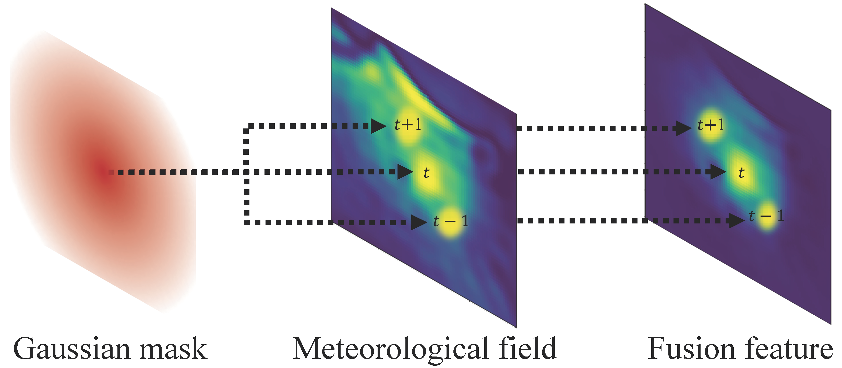
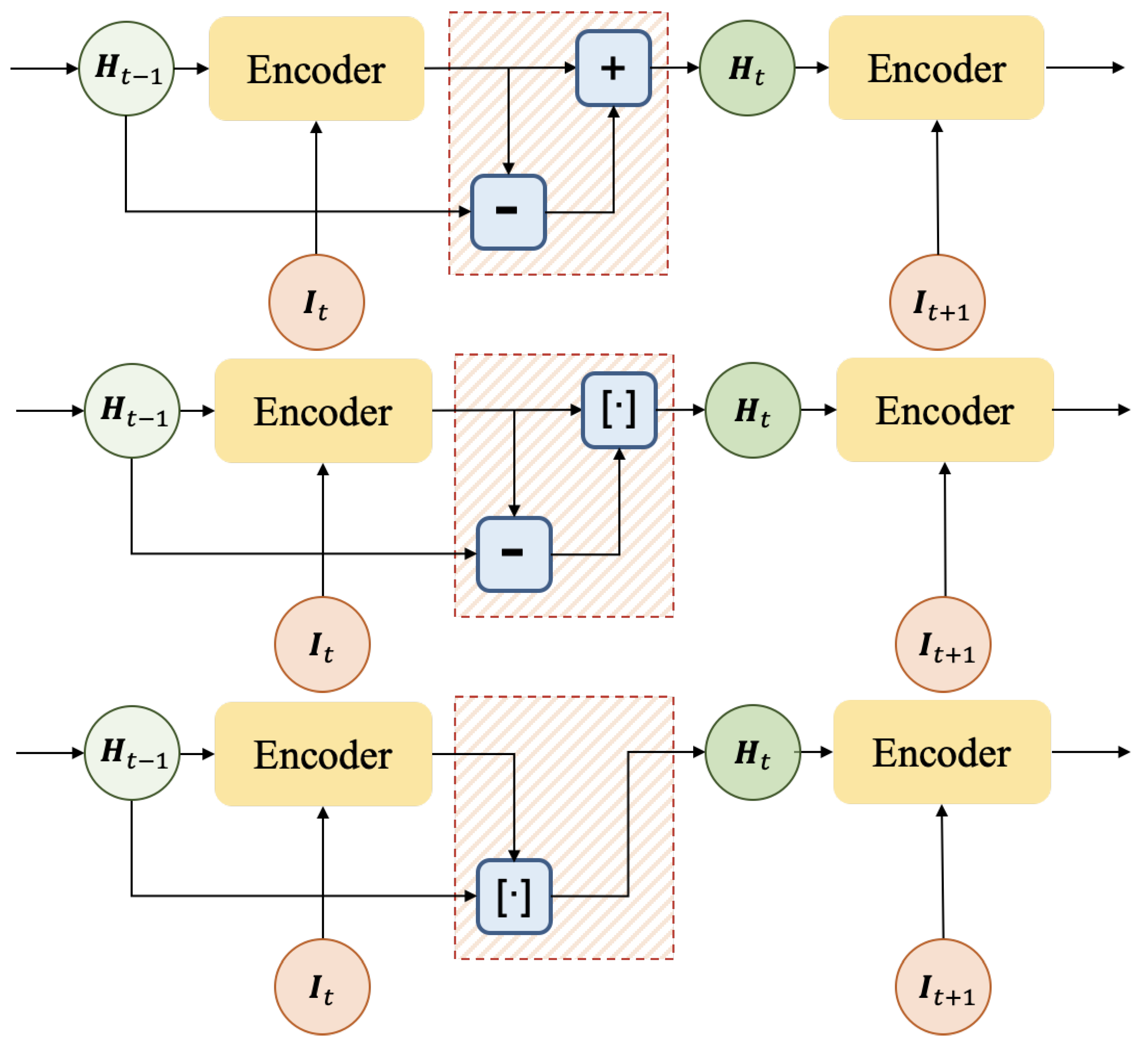
• For better feature alignment and fusion, we design a Spatial Alignment Feature Fusion (SAFF) module that preserves spatial correspondence. This fusion method can ensure that the location and the field are aligned in the spatio-temporal dimension, which is more reasonable than the existing connection methods.
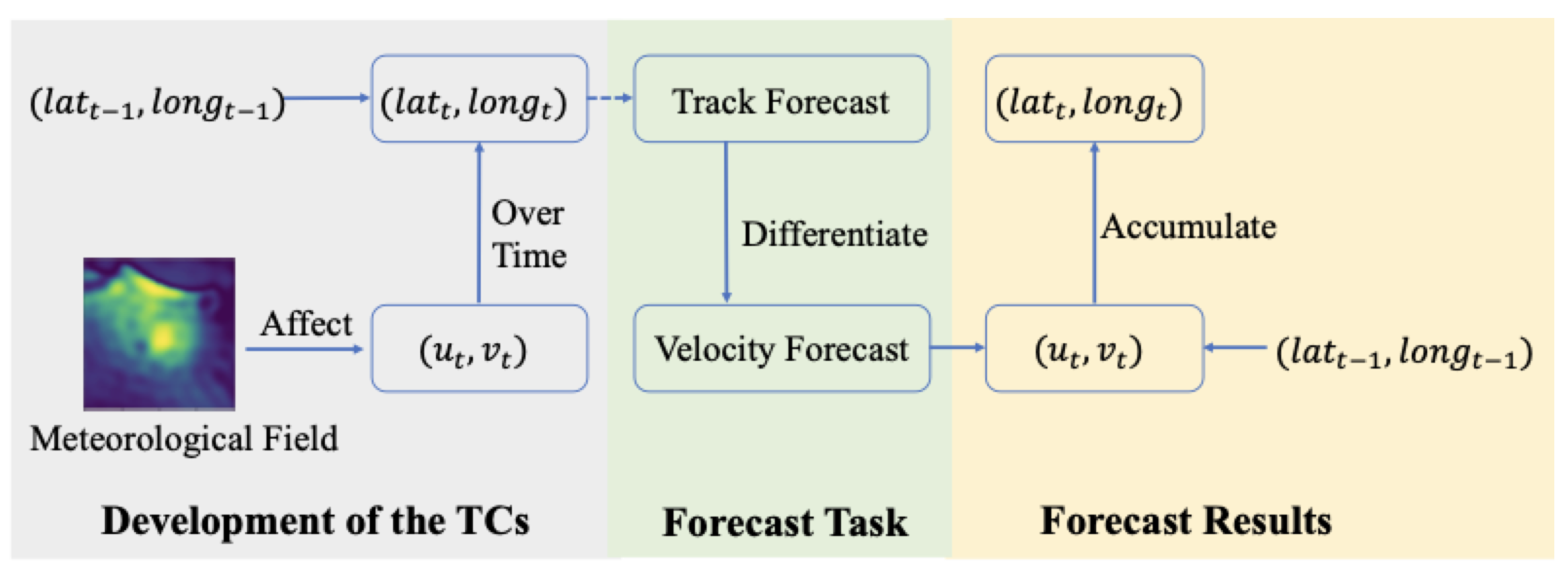
• For better forecast accuracies, we propose a Track-to-Velocity (T2V) module. We convert the track forecast into a velocity forecast. Such conversion can reduce the prediction difficulty and improve the prediction accuracy.
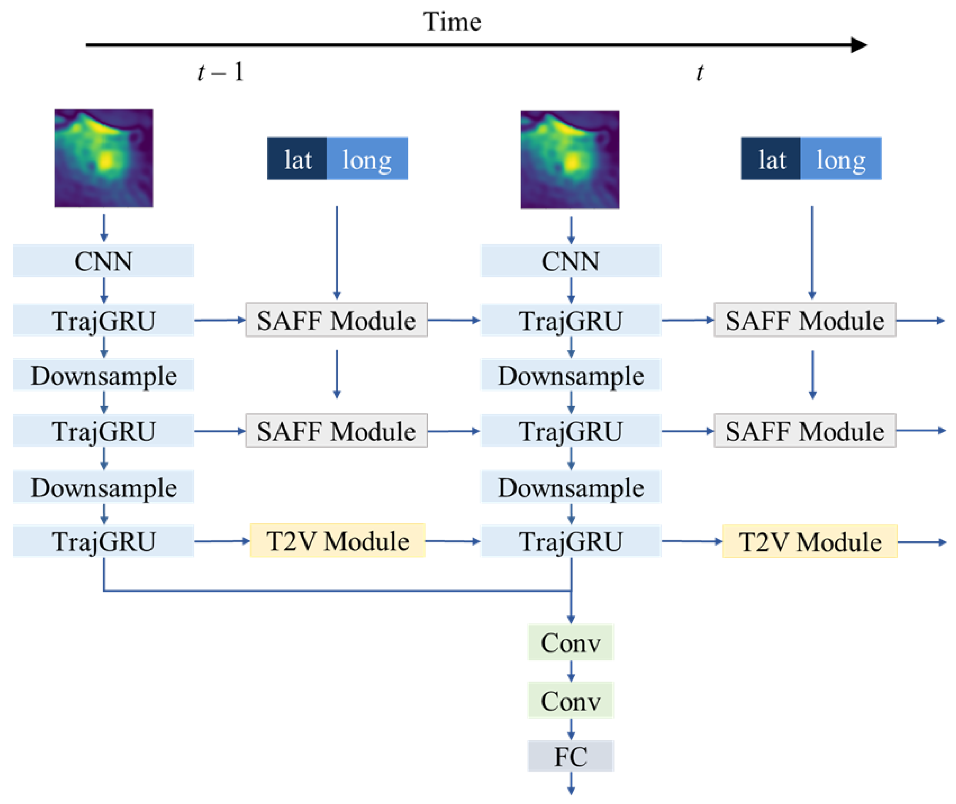
• We propose an overall framework, TC-TrajGRU, based on the SAFF and T2V modules. It presents accurate and robust forecast results. Our forecast accuracy is competitive with the NWP method in the 12 h forecast task.

2. Methodology

2.1. Spatial Alignment Feature Fusion Module

We use the location of the TC and meteorological field as input. The obstacle for feature fusion is that the feature dimensions of two kinda of data are different. We propose a Spatial Alignment Feature Fusion (SAFF) module, realizing the fusion of different dimensions. Specifically, in order to preserve the spatial correspondence, we keep the dimension of the fields but enlarge the dimension of the location. We design a dimension-increasing function for the current location ($lat$, $long$):

$$m=\exp (-(\frac{{(x-lat)}^2}{2{\sigma }^2}+\frac{{(y-long)}^2}{2{\sigma }^2})),$$

(1)

where m is the two-dimensional feature calculated by a Gaussian function, which is called the Gaussian mask. (x, and y) represents the positions on the mask. $\sigma$ depends on experience selection. We choose the Gaussian function for three reasons: (i) The mean value of the Gaussian distribution is (lat, long); that is, the mask retains the location information. (ii) The Gaussian mask shares a similar distribution to values in the field. For example, the pressure field is the lowest at (lat, long), and the value gradually increases as it is farther away. (iii) The Gaussian map is a common distribution in the fields of mathematics and physics. In addition, it is simple to implement. In addition, although the Earth is an elliptical sphere, it can be roughly deemed as a plane in the local area. Thus, we use the same $\sigma$ in the equation for simplification.

We perform fusion by multiplying the Gaussian mask with the field feature. This process preserves spatial correspondence and is illustrated in Figure 1. Our fusion method aligns the center of the Gaussian distribution with the the TC’s eye, highlighting the values around this area in the field. As a result, location information is implicitly conveyed in the fused feature. The multiplication is conducted using the Hadamard product.

2.2. Track-to-Velocity Module

Meteorological conditions impact the speed at which tropical cyclones (TCs) move and influence their trajectory over time. To predict the path of a TC, it is easier to forecast its velocity than the track itself, as track distance is merely the integral of velocity. To achieve this, we transform the task of track forecasting into a velocity prediction task, where the model’s output is the velocity ($u_t$, $v_t$) represented by the difference between adjacent (lat, long) moments:

$$(u_t,v_t)=(la{t}_t-la{t}_{t-1},lon{g}_t-lon{g}_{t-1}).$$

(2)

To obtain the track forecast result, we first record the coordinates ($la{t}_{t-1}$, $lon{g}_{t-1}$), and then accumulate the values of ($u_t$, $v_t$). By computing the difference and accumulation between these values, we can convert the track forecast and velocity forecast. This entire process is illustrated in Figure 2. Given that the distance travelled by a typhoon is relatively small compared to the size of the Earth, we approximate the Earth’s surface considering it as a plane in a local area. Hence, we represent its longitude and latitude positions using the coordinates ($u_t$, $v_t$).

To calculate the output, which measures the change in location over time, our forecast model includes a differential module called the Track-to-Velocity (T2V) module. This module differentiates the features represented by $H_t$. As mentioned earlier, the location is encoded within the fused features, enabling the difference to reveal velocity information.

We developed three differential time series structures, which enable us to attain the T2V module depicted in Figure 3. The encoder is responsible for extracting features by encoding input $I_t$ into feature $H_t^{\prime }$ derived from $H_{t-1}$. Once this is complete, the feature $H_t$ is attained by performing either a direct or indirect difference calculation within the T2V module.

The calculation formulation for structure A is as follows:

$$H_t=H_t^{\prime }+(H_t^{\prime }-H_{t-1}).$$

(3)

The calculation formulation for structure B is as follows:

$$H_t=\mathrm{Conv}[H_t^{\prime },(H_t^{\prime }-H_{t-1})],$$

(4)

where [·,·] denotes connected in series and Conv is the convolution operation.

Structure C is a simplified version of structure B. The calculation formulation is as follows:

$$H_t=\mathrm{Conv}[H_t^{\prime },H_{t-1}].$$

(5)

We demonstrate through empirical evidence that structure B outperforms the remaining two structures. Our assumption is that additional convolutional layers within this structure serve to enhance the track difference information. Specifically, convolution occurs on the concatenation of $H_t^{\prime }$ and $H_t^{\prime }-H_{t-1}$ within structure B. Within this example, $H_t^{\prime }$ and $H_t^{\prime }-H_{t-1}$ are of the same spatial shape. Their subtraction denotes the track difference, or velocity.

2.3. Overall Structure of TC-TrajGRU

To take advantage of the developments in the TC period, we apply past TC data. The TC data, as well as input, consist of two parts, the locations, denoted as $D_l$ and the meteorological fields, denoted as $D_f$, as below:

$$D_l=\{(la{t}_{t-T},lon{g}_{t-T}),...,(la{t}_{t-1},lon{g}_{t-1}),(la{t}_t,lon{g}_t)\},$$

(6)

$$D_f=\{F_{t-T},...,F_{t-1},F_t\},$$

(7)

where T is the selected timing length. We empirically set the value of T to 7 for sufficient information on early phases.

We set the task of this article as a 24 h track forecast at 6 h frequency. Since we converted the track forecast into a velocity forecast with the T2V module, the output is as follows:

$$o=\{(u_{t+1},v_{t+1}),(u_{t+2},v_{t+2}),...,(u_{t+4},v_{t+4})\},$$

(8)

where t + 1 represents t + 6 h and so on. Then, we calculated the track forecast result by accumulating the o with the current location ($la{t}_t$, $lon{g}_t$), until ($la{t}_{t+4}$, $lon{g}_{t+4}$).

$$(la{t}_{t+1},lon{g}_{t+1})=(la{t}_t+u_{t+1},lon{g}_t+v_{t+1}),$$

(9)

$$(la{t}_{t+2},lon{g}_{t+2})=(la{t}_{t+1}+u_{t+2},lon{g}_{t+1}+v_{t+2}).$$

(10)

We first constructed a model that could handle the input data $D_l$ and $D_f$, which produced the forecast result o for the velocity. To accomplish this, we utilized the SAFF module for feature fusion and the T2V module for task conversion. Specifically, we incorporated TrajGRU [15] as the backbone for its ability to extract spatio-temporal features from $D_f$, including the calculation of optical flow, which represents the trajectory of TCs in the fields and is instrumental in track forecasting. The hidden state $H_t$ of TrajGRU is fused with the input $D_l$ in the SAFF module, and, at a deeper layer, the expressive state $H_t$ and $H_{t-1}$ are used to calculate the velocity forecast via the difference calculation. The structure of the forecast model is depicted in Figure 4 and is referred to as TC-TrajGRU.

The reason for embedding the modules in TC-TrajGRU is four-fold: First, the SAFF module is placed in shallower layers of the backbone as deeper layers abbreviate feature size and decrease precision of the Gaussian mask’s location information. Second, the T2V module is integrated singularly, where location differentiation provides velocity information, and hidden states are differentiated once in T2V. Third, T2V is embedded in deeper layers where states are more representative and can be refined by previous layers. Finally, the SAFF and T2V modules are not embedded in the same layer to avoid confusion in calculating $H_t$. These modules are used sequentially, with SAFF focusing on the typhoon area first and T2V used for velocity estimation, hence their separation in different layers.

3. Experiments

3.1. Dataset

Tropical cyclone forecasting relies on remote sensing data. There are many other valuable remote sensing datasets. For example, there are some high-quality datasets for object detection [16,17,18,19,20], semantic segmentation [21,22,23,24,25], and instance segmentation [26,27,28,29,30]. These datasets contribute a lot to the overall remote sensing field. As for TC forecasting tasks, the most closely related factors are the historical tracks of TCs and the relevant reanalyzed meteorological field variables, which have relatively higher temporal resolution and consistency. Hence, we selected the above two types of data for model training and testing.

3.1.1. The Track of TCs

The dataset [31] consists of 182 tracks of tropical cyclones in the NIO basin spanning from 1979 to 2018. The dataset was sourced from the NIO best track dataset [31] organized by the Joint Typhoon Warning Center and includes the location of the TC eyes every 0 h, 6 h, 12 h, and 18 h for each TC data point. To construct the input of our model, we used the sliding window method. Across all 182 TCs, we obtained a total of 2528 samples $D_l$ and corresponding forecast labels. To account for the annual variability in TCs, the data were separated into training and testing sets by year, as shown in

Table 1. The division of dataset. # means the amount.

Data	Training Set	Testing Set
Year	1979–2014	2015–2018
# TCs	160	22
# Samples	2294	234

.

3.1.2. The Sea Level Pressure Field

As TCs are low-pressure vortices, the input for our analysis of their structure is the sea level pressure (SLP) field. There are various ways to obtain historical sea level pressure data, including datasets like ERA5 [32] released by the European Centre for Medium-Range Weather Forecasts (ECMWF) and the climate forecast system reanalysis (CFSR) data [33] released by NOAA NWS National Centers for Environmental Prediction (NCEP). We obtained these fields from the CFSR reanalysis. This dataset is widely used in climate research and includes multiple meteorological variables, such as wind and temperature. The CFSR data cover the globe from 1979 onwards and have a resolution of $0.5^{\circ }$ with measurements taken at 0 h, 6 h, 12 h, and 18 h daily. To analyze a specific TC, we extracted the SLP field of the surrounding area at each time step during the period of interest. At time t, the SLP field is a ${40}^{\circ }\mathrm{N}\times {40}^{\circ }\mathrm{E}$ grid ($80\times 80$ pixels) centered on the current location of the TC.

We split the dataset by using the data gathered before 2018 for training, while the data from between 2019 and 2021 were reserved for testing the model.

3.2. Metrics

One metric to evaluate performance involves measuring the distance between the predicted coordinates ($la{t}_{t+i}$ and $lon{g}_{t+i}$) and the ground truth on the Earth’s surface for i = 1, 2, 3, 4 representing forecast biases of 6 h, 12 h, 18 h, and 24 h. The performance of the forecast model is evaluated using the mean distance of all test samples as follows, where $n\in N$ enumerates all test samples:

$$d_{t+i}=\frac{{\sum }_n^N{d}_{n,t+i}}{N},i=\{1,2,3,4\}.$$

(11)

Given that the tracks of TCs are mainly influenced by their direction of movement, we assessed the robustness of the model in anticipating this factor. To this end, we utilized evaluation metrics employed in NWP techniques as a benchmark, as follows:

$$s_{t+i}=\frac{{\sum }_n^N{o}_{n,t+i}}{N}\times 100\%,$$

(12)

where

$$o_{n,t+i}=\left\{\begin{array}{cc}\hfill 1,& \mathrm{if}\mathrm{the}\mathrm{forecast}\mathrm{is}\mathrm{in}\mathrm{the}\mathrm{correct}\mathrm{direction};\hfill \\ \hfill 0,& \mathrm{else}.\hfill \end{array}\right.$$

We divided the direction into four distinct areas, and any prediction that falls within these areas is considered to be correct. The accuracy of our forecast improves as the value of $s_{t+i}$ increases, indicating a better performance from our model.

3.3. Experiment Setting and Training Details

We utilized the Adam optimizer [34] and configured the initial learning rate to 1 $\times {10}^{-3}$, with a gradual decrease to 1 $\times {10}^{-4}$ following a cosine schedule. Our models underwent 60 training epochs to achieve optimal performance. The input has a time length of 8, spanning from time t − 7 (42 h in the past) to the present time t. Meanwhile, the output has a timing length of 4, starting from t + 1 and continuing up to t + 4. We computed the training back-propagation error as the average loss of these four moments, employing the MSELoss function.

3.4. Network Details

In

Table 2. Detailed structure of the network.

Module	Layer	Output Shape (C, H, W)
Encoder	Conv	(8, 96, 96)
	TC-TrajGRU	(64, 96, 96)
	Conv	(192, 32, 32)
	TC-TrajGRU	(192, 32, 32)
	Conv	(192, 16, 16)
	TrajGRU	(192, 16, 16)
Forecaster	Conv	(96, 14, 14)
	Conv	(48, 12, 12)
	Conv	(24, 10, 10)
	Conv	(12, 6, 6)
	Conv	(4, 2, 2)
	FC	(4, 2)

, we illustrate the details about the network in terms of the layers and output shapes of each layer. The network consists of the encoder and the forecaster. In the encoder, it contains three sequential pairs of convolutional layers and TC-TrajGRU. The structure of TC-TrajGRU is illustrated in Figure 4. In the forecaster, there are five convolutional layers and one fully connected layer for output. It output (4, 2) features, representing velocities in the x, y directions for 6 h, 12 h, 18 h, and 24 h.

3.5. Comparison Experiments

In comparative experiments, three types of input and corresponding forecast models were utilized. (i) The input comprises solely of TC tracks. Since there exists no spatial dimension, an original LSTM was employed to forecast the location directly. (ii) The input comprises solely the SLP field. TrajGRU is utilized for velocity forecast and then accumulated with the recorded location of the current time to generate the forecast track, which is then compared with our method. (iii) The input includes both tracks and fields. Our model, TC-TrajGRU, is implemented to forecast the velocity, where TC-TrajGRU without the T2V module is referenced as TC-TrajGRU, whereas the TC-TrajGRUs with three different T2V modules are denoted as TC-TrajGRU-a, TC-TrajGRU-b, and TC-TrajGRU-c. Additionally, the 24 h forecast error of the Fusion Network [10] is listed for comparison. The mean distance of the forecast results is reported in

Table 3. Results of different method, where the metrics in bold are the best.

Models	Mean Distance of Forecast Result/km
	6 h	12 h	18 h	24 h
LSTM	29.7	62.5	101.2	145.2
TrajGRU	35.0	81.0	106.9	150.8
Fusion Net [10]	-	-	-	138.9
TC-TrajGRU	28.3	58.9	93.9	130.5
TC-TrajGRU-a	27.7	56.2	88.4	122.7
TC-TrajGRU-b	26.7	53.1	83.7	116.6
TC-TrajGRU-c	26.1	53.7	84.4	117.7

. Although the testing set utilized by the Fusion Network may differ from ours, they share the same ocean for a fair comparison.

In Table 3, the forecast performance of the Fusion Network and all TC-TrajGRU models surpasses that of LSTM and TrajGRU. This highlights the significance of utilizing both tracks and fields in the prediction process. Furthermore, the TC-TrajGRU models outperform the Fusion Network models, indicating the superior performance of the SAFF module over feature concatenation. The incorporation of the T2V module further reduces the mean distances in the TC-TrajGRU models. This suggests the effectiveness of the T2V module. Notably, structure (b) and (c) of the T2V module exhibit greater performance improvements than structure (a). We speculate that the additional convolution in the calculation process of structure (b) and (c) enhances the model’s representation ability by making the difference calculation more adaptive.

3.6. Evaluation of Directional Forecast Stability

We assessed the stability of the forecast model in predicting the direction of movement. Our evaluation utilized TC-TrajGRU-b and TC-TrajGRU-c, which are the top-performing models identified in Table 3. The level of stability across different forecast horizons is presented in

Table 4. Stability of different models.

Models	Directional Stability
	6 h	12 h	18 h	24 h
TC-TrajGRU-b	88.3%	84.4%	83.5%	81.4%
TC-TrajGRU-c	88.3%	83.1%	81.8%	77.1%

. Our models deliver consistent predictions in terms of movement direction. However, the level of directional stability reduces as the forecast timeline extends.

The definition of directional stability is the proportion of predictions with the right direction among the total predictions. It is true that as the forecast timeline increases, the prediction gradually becomes harder. However, the stability degradation is limited, especially for TC-TrajGRU-b. In the 24 h forecast, more than 80% of the prediction has the right direction, which is an acceptable and promising results.

3.7. Annual Comparison with Official Track Forecast

The India Meteorological Department (IMD) is responsible for predicting and alerting about tropical cyclones in the Northern Indian Ocean (NIO) region. The IMD employs advanced forecasting methods including NWP models and ensemble techniques, which offer the highest level of prediction accuracy. To evaluate our model, we compared it with IMD’s annual forecast [35]. In the 12 h forecast task, both TC-TrajGRU-b and TC-TrajGRU-c show comparable performance to IMD’s official forecast. However, our models significantly underperform IMD’s in the 24 h forecast task.

In

Table 5. Annual comparison with official track forecast, the bold are the best. # means the amount.

Year		2015	2016	2017	2018
# TCs		5	5	4	8
Mean distance of 12 h forecast/km	TC-TrajGRU-b	50.4	56.3	55.7	50.7
	TC-TrajGRU-c	52.2	59.1	56.6	49.5
	IMD	54.7	59.7	43.7	55.4
Mean distance of 24 h forecast/km	TC-TrajGRU-b	113.7	111.53	141.5	110.4
	TC-TrajGRU-c	119.6	120.8	137.8	108.4
	IMD	94.4	96.1	61.4	87.5

, we find that our model presents better forecast accuracies than the strong IMD system, for example in 2015, 2016, and 2018. This shows the effectiveness of our methods. In the 24 h forecast, our results are inferior to those of IMD. We suppose that the reason behind this is the data distribution. We would like to collect more data that focus on 24 h and longer, which would improve our results on 24 h.

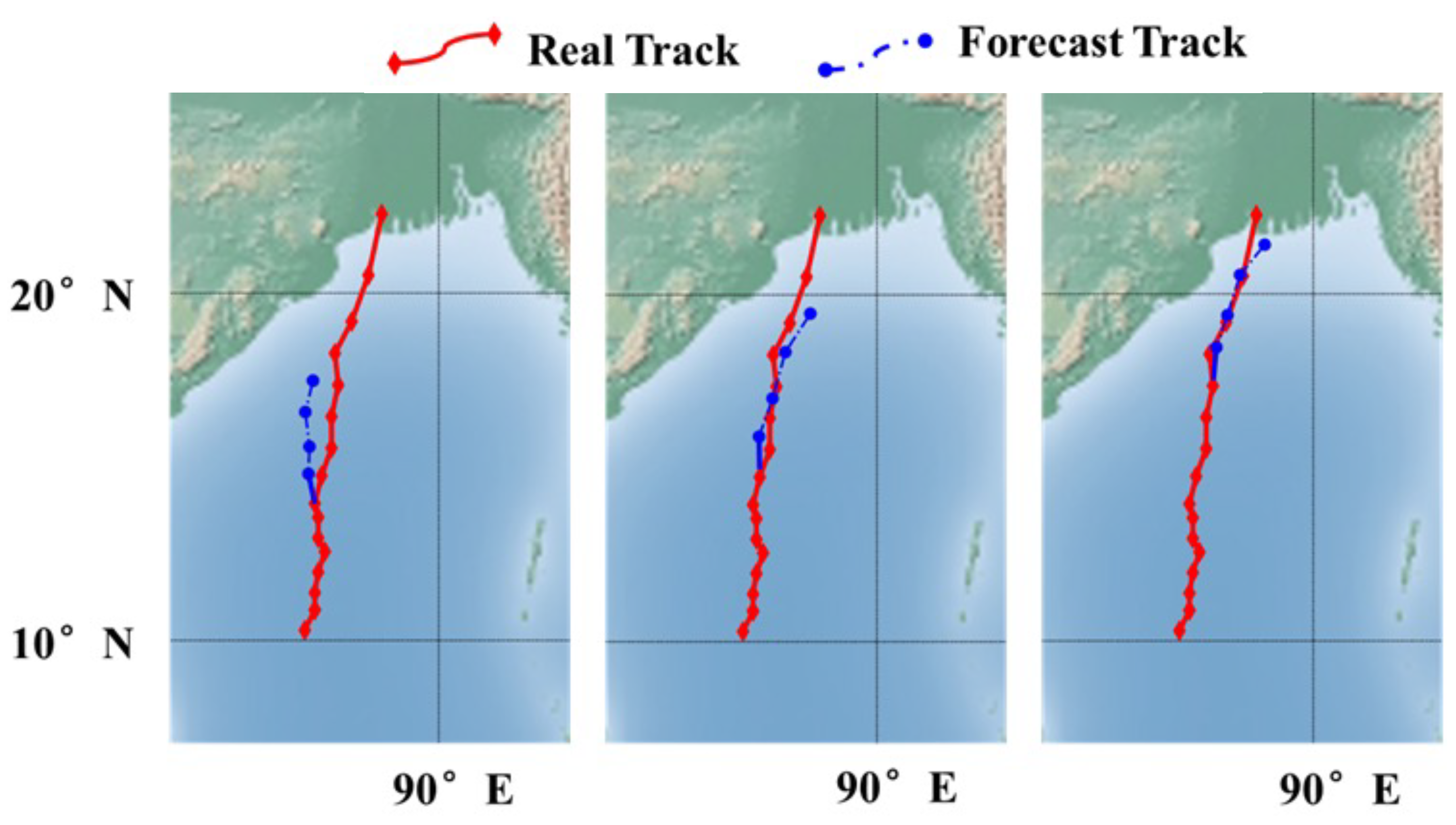
3.8. Forecast Examples

We have chosen the 2020 formation of TC Amphan to illustrate our point.

Table 6. Forecast examples of the proposed method on the TC Amphan.

Forecast Time	Distance/km
	6 h	12 h	18 h	24 h
18 May 2020 06:00	60.7	74.6	121.9	114.2
18 May 2020 12:00	42.4	70.7	84.7	81.2
19 May 2020 12:00	30.4	22.8	9.8	94.9

and Figure 5 demonstrate the forecast time and distance covered by the TC. The distance is determined by the direction and speed deviations. As the TC approaches land, the distance usually increases due to environmental complexity.

In Figure 5, there are three example sub-figures, where we change the starting points for forecasting. It shows that as the starting point moves closer to the land, the prediction becomes more accurate. This makes our model practical and useful, as we care more about the coastal area in real applications. The reason behind this relates to the data collection, as the coastal tracks are easier to observe well.

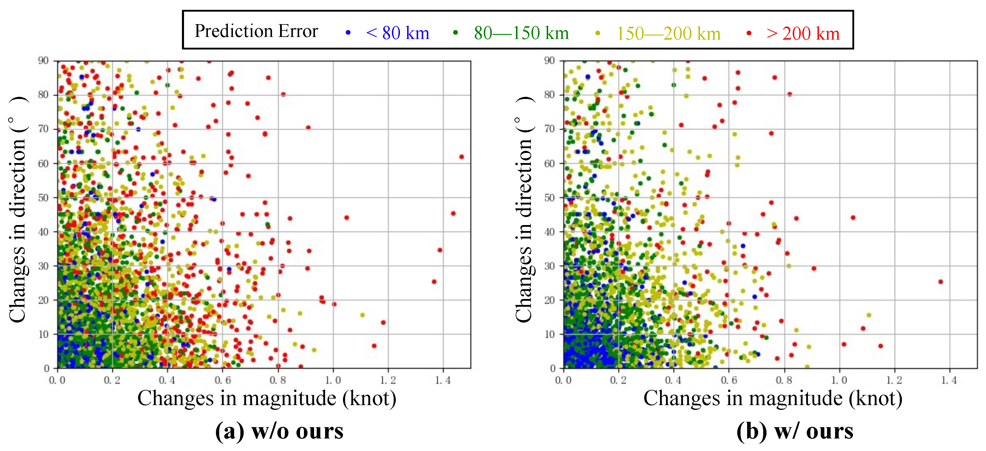
3.9. Prediction Errors

In Figure 6, we visualize the effects of our methods on prediction errors, alongside changes in directions and magnitudes. We split the prediction errors into four ranges: <80 km, 80–150 km, 150–200 km, and >200 km. As shown in the figure, as the changes in direction or magnitudes increase, the prediction difficulty grows. With our methods, there are more predictions with controllable small errors (<80 km) and less predictions with very large errors (>200 km). This detailed visualization shows the effectiveness of our method.

4. Conclusions

This article presents a dual approach to enhance TC track forecasts. Firstly, the paper incorporates a Spatial Alignment Feature Fusion module into the forecast network to improve feature fusion. Secondly, a Track-to-Velocity module is included in the output aspect to simplify forecasting. Through experiments, the paper demonstrates the effectiveness and robustness of the modules. Notably, the results are comparable to the official forecast for the 12 h forecast task.

References

1. Pickle, J.D. Forecasting Short-Term Movement and Intensification of Tropical Cyclones Using Pattern-Recognition Techniques; Phillips Laboratory, Directorate of Geophysics, Air Force Systems Command: Chestertown, MD, USA, 1991. [Google Scholar]
2. Ali, M.M.; Kishtawal, C.M.; Jain, S. Predicting cyclone tracks in the north Indian Ocean: An artificial neural network approach. Geophys. Res. Lett. 2007, 34, 4. [Google Scholar] [CrossRef]
3. Wang, Y.; Zhang, W.; Fu, W. Back Propogation(BP)-neural network for tropical cyclone track forecast. In Proceedings of the 2011 19th International Conference on Geoinformatics, Shanghai, China, 24–26 June 2011; pp. 1–4. [Google Scholar]
4. Kordmahalleh, M.M.; Sefidmazgi, M.G.; Homaifar, A. A Sparse Recurrent Neural Network for Trajectory Prediction of Atlantic Hurricanes. In Proceedings of the Genetic Evolutionary Computation Conference, Denver, CO, USA, 20–24 July 2016. [Google Scholar]
5. Alemany, S.; Beltran, J.; Pérez, A.; Ganzfried, S. Predicting Hurricane Trajectories using a Recurrent Neural Network. In Proceedings of the Association for the Advancement of Artificial Intelligence, Honolulu, HI, USA, 27 January–1 February 2019. [Google Scholar]
6. Gao, S.; Zhao, P.; Pan, B.; Li, Y.; Zhou, M.; Xu, J.; Zhong, S.; Shi, Z.X. A nowcasting model for the prediction of typhoon tracks based on a long short term memory neural network. Acta Oceanol. Sin. 2018, 37, 8–12. [Google Scholar] [CrossRef]
7. Song, T.; Li, Y.; Meng, F.; Xie, P.; Xu, D. A Novel Deep Learning Model by BiGRU with Attention Mechanism for Tropical Cyclone Track Prediction in Northwest Pacific. J. Appl. Meteorol. Climatol. 2022, 61, 3–12. [Google Scholar] [CrossRef]
8. Mudigonda, M.; Kim, S.; Mahesh, A.; Kahou, S.E.; Kashinath, K.; Williams, D.N.; Michalski, V.; O’Brien, T.; Prabhat, M. Segmenting and Tracking Extreme Climate Events using Neural Networks. Deep Learning for Physical Sciences Workshop. In Proceedings of the NIPS Conference, Long Beach, CA, USA, 4–9 December 2017. [Google Scholar]
9. Kim, S.; Kim, H.; Lee, J.; Yoon, S.; Kahou, S.E.; Kashinath, K.; Prabhat. Deep-Hurricane-Tracker: Tracking and Forecasting Extreme Climate Events. In Proceedings of the 2019 IEEE Winter Conference on Applications of Computer Vision (WACV), Waikoloa, HI, USA, 7–11 January 2019; pp. 1761–1769. [Google Scholar]
10. Giffard-Roisin, S.; Yang, M.; Charpiat, G.; Kumler-Bonfanti, C.; K’egl, B.; Monteleoni, C. Tropical Cyclone Track Forecasting Using Fused Deep Learning from Aligned Reanalysis Data. Front. Big Data 2020, 3, 1. [Google Scholar] [CrossRef]
11. Shi, X.; Chen, Z.; Wang, H.; Yeung, D.Y.; Wong, W.K.; Chun Woo, W. Convolutional LSTM Network: A Machine Learning Approach for Precipitation Nowcasting. In Proceedings of the Advances in Neural Information Processing Systems, Montréal, QC, Canada, 7–12 December 2015. [Google Scholar]
12. Liu, Z.; Hao, K.; Geng, X.; Zou, Z.; Shi, Z. Dual-Branched Spatio-Temporal Fusion Network for Multihorizon Tropical Cyclone Track Forecast. IEEE J. Sel. Top. Appl. Earth Obs. Remote Sens. 2022, 15, 3842–3852. [Google Scholar] [CrossRef]
13. Bi, K.; Xie, L.; Zhang, H.; Chen, X.; Gu, X.; Tian, Q. Accurate medium-range global weather forecasting with 3D neural networks. Nature 2023, 619, 533–538. [Google Scholar] [CrossRef] [PubMed]
14. Chen, K.; Han, T.; Gong, J.; Bai, L.; Ling, F.; Luo, J.J.; Chen, X.; Ma, L.; Zhang, T.; Su, R.; et al. FengWu: Pushing the Skillful Global Medium-range Weather Forecast beyond 10 Days Lead. arXiv 2023, arXiv:2304.02948. [Google Scholar]
15. Shi, X.; Gao, Z.; Lausen, L.; Wang, H.; Yeung, D.Y.; Wong, W.K.; Woo, W.C. Deep Learning for Precipitation Nowcasting: A Benchmark and A New Model. arXiv 2017, arXiv:1706.03458. [Google Scholar]
16. Andle, J.; Soucy, N.; Socolow, S.; Sekeh, S.Y. The Stanford Drone Dataset Is More Complex Than We Think: An Analysis of Key Characteristics. IEEE Trans. Intell. Veh. 2023, 8, 1863–1873. [Google Scholar] [CrossRef]
17. Mundhenk, T.N.; Konjevod, G.; Sakla, W.A.; Boakye, K. A Large Contextual Dataset for Classification, Detection and Counting of Cars with Deep Learning. In Proceedings of the Computer Vision—ECCV 2016—14th European Conference, Amsterdam, The Netherlands, 11–14 October 2016; Leibe, B., Matas, J., Sebe, N., Welling, M., Eds.; Springer: Berlin/Heidelberg, Germany, 2016; Volume 9907, pp. 785–800. [Google Scholar] [CrossRef]
18. Lam, D.; Kuzma, R.; McGee, K.; Dooley, S.; Laielli, M.; Klaric, M.; Bulatov, Y.; McCord, B. xView: Objects in Context in Overhead Imagery. arXiv 2018, arXiv:1802.07856. [1802.07856]. [Google Scholar]
19. Weinstein, B.G.; Marconi, S.; Bohlman, S.A.; Zare, A.; Singh, A.; Graves, S.J.; White, E.P. A remote sensing derived data set of 100 million individual tree crowns for the National Ecological Observatory Network. eLife 2021, 10, e62922. [Google Scholar] [CrossRef] [PubMed]
20. Gasienica-Józkowy, J.; Knapik, M.; Cyganek, B. An ensemble deep learning method with optimized weights for drone-based water rescue and surveillance. Integr. Comput. Aided Eng. 2021, 28, 221–235. [Google Scholar] [CrossRef]
21. Rahnemoonfar, M.; Chowdhury, T.; Sarkar, A.; Varshney, D.; Yari, M.; Murphy, R.R. FloodNet: A High Resolution Aerial Imagery Dataset for Post Flood Scene Understanding. IEEE Access 2021, 9, 89644–89654. [Google Scholar] [CrossRef]
22. Wang, J.; Zheng, Z.; Ma, A.; Lu, X.; Zhong, Y. LoveDA: A Remote Sensing Land-Cover Dataset for Domain Adaptive Semantic Segmentation. In Proceedings of the Neural Information Processing Systems Track on Datasets and Benchmarks 1, NeurIPS Datasets and Benchmarks, Online, 21 August 2021. [Google Scholar]
23. Castillo-Navarro, J.; Saux, B.L.; Boulch, A.; Audebert, N.; Lefèvre, S. Semi-supervised semantic segmentation in Earth Observation: The MiniFrance suite, dataset analysis and multi-task network study. Mach. Learn. 2022, 111, 3125–3160. [Google Scholar] [CrossRef]
24. Azimi, S.M.; Henry, C.; Sommer, L.; Schumann, A.; Vig, E. SkyScapes—Fine-Grained Semantic Understanding of Aerial Scenes. In Proceedings of the 2019 IEEE/CVF International Conference on Computer Vision, ICCV, Seoul, Republic of Korea, 27 October–2 November 2019; pp. 7392–7402. [Google Scholar] [CrossRef]
25. Baetens, L.; Desjardins, C.; Hagolle, O. Validation of Copernicus Sentinel-2 Cloud Masks Obtained from MAJA, Sen2Cor, and FMask Processors Using Reference Cloud Masks Generated with a Supervised Active Learning Procedure. Remote Sens. 2019, 11, 433. [Google Scholar] [CrossRef]
26. Garnot, V.S.F.; Landrieu, L. Panoptic Segmentation of Satellite Image Time Series with Convolutional Temporal Attention Networks. In Proceedings of the 2021 IEEE/CVF International Conference on Computer Vision, ICCV 2021, Montreal, QC, Canada, 10–17 October 2021; pp. 4852–4861. [Google Scholar] [CrossRef]
27. Shermeyer, J.; Hossler, T.; Etten, A.V.; Hogan, D.; Lewis, R.; Kim, D. RarePlanes: Synthetic Data Takes Flight. In Proceedings of the IEEE Winter Conference on Applications of Computer Vision, WACV 2021, Waikoloa, HI, USA, 3–8 January 2021; pp. 207–217. [Google Scholar] [CrossRef]
28. Chiu, M.T.; Xu, X.; Wei, Y.; Huang, Z.; Schwing, A.G.; Brunner, R.; Khachatrian, H.; Karapetyan, H.; Dozier, I.; Rose, G.; et al. Agriculture-Vision: A Large Aerial Image Database for Agricultural Pattern Analysis. In Proceedings of the 2020 IEEE/CVF Conference on Computer Vision and Pattern Recognition, CVPR 2020, Seattle, WA, USA, 13–19 June 2020; pp. 2825–2835. [Google Scholar] [CrossRef]
29. Zamir, S.W.; Arora, A.; Gupta, A.; Khan, S.H.; Sun, G.; Khan, F.S.; Zhu, F.; Shao, L.; Xia, G.; Bai, X. iSAID: A Large-scale Dataset for Instance Segmentation in Aerial Images. In Proceedings of the IEEE Conference on Computer Vision and Pattern Recognition Workshops, CVPR Workshops 2019, Long Beach, CA, USA, 16–20 June 2019; pp. 28–37. [Google Scholar]
30. Gupta, R.; Goodman, B.; Patel, N.; Hosfelt, R.; Sajeev, S.; Heim, E.; Doshi, J.; Lucas, K.; Choset, H.; Gaston, M. Creating xBD: A Dataset for Assessing Building Damage from Satellite Imagery. In Proceedings of the IEEE/CVF Conference on Computer Vision and Pattern Recognition (CVPR) Workshops, Long Beach, CA, USA, 16–20 June 2019. [Google Scholar]
31. Chu, J.H.; Levine, A.D.S. North Indian Ocean Best Track Data. Available online: https://www.metoc.navy.mil/jtwc/jtwc.html?north-indian-ocean (accessed on 25 June 2023).
32. Hersbach, H.; Bell, B.; Berrisford, P.; Hirahara, S.; Horányi, A.; Muñoz-Sabater, J.; Nicolas, J.; Peubey, C.; Radu, R.; Schepers, D.; et al. The ERA5 global reanalysis. Q. J. R. Meteorol. Soc. 2020, 146, 1999–2049. [Google Scholar] [CrossRef]
33. Saha, S.; Moorthi, S.; Pan, H.L.; Wu, X.; Wang, J.; Nadiga, S.; Tripp, P.; Kistler, R.; Woollen, J.; Behringer, D.; et al. The NCEP Climate Forecast System Reanalysis. Bull. Am. Meteorol. Soc. 2010, 91, 1015–1057. [Google Scholar] [CrossRef]
34. Kingma, D.P.; Ba, J. Adam: A Method for Stochastic Optimization. In Proceedings of the International Conference on Learning Representations, San Diego, CA, USA, 7–9 May 2015. [Google Scholar]
35. Mohapatra, M.; Sharma, M. Cyclone warning services in India during recent years: A review. Mausam 2021, 70, 635–666. [Google Scholar] [CrossRef]
Figure 1. The diagram of spatial aligned feature fusion. Green means high values in the field and features.
Remotesensing 15 04938 g001
Figure 2. The conversion of track forecast and velocity forecast.
Remotesensing 15 04938 g002
Figure 3. Different T2V modules.
Remotesensing 15 04938 g003
Figure 4. The structure of TC-TrajGRU.
Remotesensing 15 04938 g004
Figure 5. Forecast examples.
Remotesensing 15 04938 g005
Figure 6. Ablations on prediction errors for without and with our method.
Remotesensing 15 04938 g006