Article

A Functional Zoning Method in Rural Landscape Based on High-Resolution Satellite Imagery

1
College of Horticulture and Forestry Sciences, Huazhong Agricultural University, Wuhan 430070, China
2
Hubei Engineering Technology Research Centre for Forestry Information, Huazhong Agricultural University, Wuhan 430070, China
3
Key Laboratory of Urban Agriculture in Central China, Ministry of Agriculture, Wuhan 430070, China
*
Author to whom correspondence should be addressed.
Remote Sens. 2023, 15(20), 4920; https://doi.org/10.3390/rs15204920
Submission received: 19 September 2023 / Revised: 7 October 2023 / Accepted: 9 October 2023 / Published: 12 October 2023

Abstract

:
Mapping functional zones for rural landscapes is the foundational work for rural land use planning and plays a very important role in the economic development and resource management utilization of rural areas. However, the traditional manual delineation of functional zone boundaries empirically in rural areas is labor-intensive, time-consuming, and lacks the consideration of spatial landscape patterns. The emergence of high-resolution remote sensing imagery and image segmentation has facilitated the analysis of ground landscape information and patterns, but there is still a lack of functional zone boundary mapping methods applicable to rural landscapes. To address this, we propose a functional zoning method called multiscale merging of landscape contextual and shape characteristics with heterogeneity indices (M2LHI) for mapping geographic boundaries for rural landscapes based on high-resolution remote sensing imagery. The landscape contextual features were first constructed based on the geospatial distances of landscape types, and then, the dominance index and shape index were introduced to quantify the landscape heterogeneity by object-oriented image analysis. Then, the automated merging of adjacent landscape units based on the thresholds of the landscape heterogeneity indices was performed to map the initial zones. The final rural functional zones were defined based on the main function in the zone. The study was carried out in three typical rural landscapes (hilly countryside, flat countryside, and grassland countryside) located in Fujian, Xinjiang, and Inner Mongolia, China, and the freely available Gaofen-2 (GF-2) satellite imagery was used as the data source. We compared the boundaries of mapped functional zones and reference functional zones, and the matching and inclusion ratios of the final functional zones mapped in each case were bigger than 78%, indicating that the M2LHI method has a high ability to map the functional spatial patterns. The overall accuracies of mapping functional zones with different functions were 95.9%, 89.0%, and 92.1% for the respective cases. The results demonstrated that the M2LHI method effectively quantifies landscape heterogeneity and accurately delineates functional zones with different landscape patterns. It can provide a scientific basis for rural planning and management and efficiently draw reasonable geographic boundaries for rural functional zones.

Graphical Abstract

1. Introduction

Rural regions are characterized by a complex mix of buildings and extensive natural resources, including forests, farmlands, and water resources [1,2]. A rural landscape is the product of the interaction between natural elements and human activity that occurs in time and space [3], and it represents a non-renewable resource that can provide unparalleled information about the general state of the environment. The delineation of “production–living–ecological” spaces [4,5] in rural landscapes plays an essential role in the sustainable use of natural resources and the development of rural areas. However, rapid urbanization and industrialization in the past three decades in China have prioritized urban growth, leading to practical challenges such as conflicting resource use and damage to ecology [6]. As a result, landscape resources in many rural regions remain underutilized and poorly managed. To solve these problems, functional zones have been proposed to provide a scientific basis for planning and managing the sustainable use of resources. In urban areas, the functional zone is developed to standardize the urban morphology or distinguish different precinct ventilation zones [7] and the heat island effect [8]. The same as the urban functional zone, the rural landscape functional zone aims to provide scientific management boundaries for coordinating the relationship between human life, production, and the sustainable utilization of natural ecological resources in rural areas [9,10], and it plays a very important role in the economic development and resource management utilization of rural areas. The delineation of landscape functional zones is an important issue.
Traditionally, the boundaries of rural landscapes’ functional zones have been defined by administrative delineations or hand sketches [11]. However, the former approach makes it difficult to fully consider environmental factors, which may damage natural attributes [12], and limits the geospatial scale of the functional zones [13]. It will create a mismatch between functional zones and administrative zones, which will hinder the development of the region [14]. Through imagery interpretation, human hand sketching based on field surveys can draw the fine-grained boundary of the functional zone within the village area. Even though it can provide a better reference for relevant research validation, it is time-consuming and laborious when applied to a large number of villages. When hand sketching is too much work, it is easy to make mistakes in judging the attributes and configurations of local landscape elements. As the population grows, rural regions are rapidly developing to meet the needs of the population, and activities such as agricultural expansion and intensification, industrialization, natural forest deforestation, and timber plantation occur [15,16]. These activities result in land use changes that would alter the boundaries of rural landscape functional zones. It would be very labor-intensive to still draw the boundaries of functional zones by hand drawing. Therefore, in the current era of rapid population growth, how to effectively delineate accurate functional zoning boundaries of rural landscapes is an urgent problem.
In recent years, remote sensing technology has developed rapidly and is capable of acquiring information about ground objects and regions quickly and in real-time. Satellite imagery has the advantages of multi-temporal availability, as well as large spatial coverage for monitoring, identifying, and assessing terrestrial landscape resources, such as Landsat, the Satellite for Observation of Earth (SPOT), the Moderate Resolution Imaging Spectroradiometer (MODIS), and others [17,18,19]. Satellite imagery of various resolutions has been increasingly used for mapping in urban and peri-urban environments [20], and high-resolution imagery is expert at capturing the presence and characteristics of remote rural settlements, due to small land parcels and the low density of man-made structures in these settings [21]. There are many high-resolution imagery sources (e.g., IKONOS, QuickBird, and WorldView) that are frequently used, and the Chinese Gaofen Satellites are regarded as suitable inputs for Chinese rural applications [22], as they can provide free sub-meter-level imagery of most areas in China [23], facilitating long-term and stable research and applications in rural landscapes [24]. This facilitates resource monitoring and provides the information needed to measure function in remote rural environments.
Land use and land cover (LULC) are commonly used in quantifying landscape functions and processes [25]. The visual interpretation of high-resolution imagery in the visible band to identify LULC areas for manually mapping functional zones is a common method. Land cover indices such as the normalized difference vegetation index (NDVI) and normalized difference built-up index (NDBI) are also commonly used to identify LULC areas [26,27]. The indices used in the different studies differ according to the object of study and the characteristics of the regional features. Based on suitable land cover indices, obtaining distribution information on diverse landscapes through image classification is a popular strategy used with the development of computers [28,29,30,31]. Among image classification methods, the emerging object-oriented approach is more suitable for different resolutions and classification scales than pixel-oriented classification, which can avoid the “salt and pepper” phenomenon [32]. Now, multiscale segmentation has become a key technology for extracting raster information with a high spatial resolution, which can produce polygonal objects with minimum heterogeneity and maximum homogeneity at any scale with minimal loss of image information [33]. Image objects have strong advantages in geometric metrics [34], neighborhood analysis [35], and spatial morphology analysis [36], which are important for planning landscape functional zones. However, object segmentation is designed to obtain homogenous image objects [37], but functional zones are generally composed of various geographic objects [13,38]. Landscape functional zoning involves reclassifying landscape units based on natural environmental characteristics and requires focusing on the primary functions of the region while coordinating the spatial arrangement of different landscape types [13,38]. Functional zones usually need to be determined by considering the spatial morphology and structural analysis of landscape units [11,39]. They are not only spatially larger than objects, but also differ in scale, so traditional object-based methods cannot directly map the boundaries of functional zones [40]. Pixel-based classification often results in fragmented classification patches that do not meet the requirements of highly intensively managed functional zones [41]. Therefore, implementing the drawing from pixels or objects to functional zones is a great need.
To address this issue, mapping functional zones by grouping nearby objects with the same function is presented. Such an object-based functional zone mapping was proven to be feasible and successfully applied in urban areas [42]. When merging adjacent units to obtain functional zones, constructing suitable landscape indices is a critical task for functional zoning. Landscape heterogeneity is the basis for functional zone mapping [43]. Regarding the monitoring and management of landscape resources, the identification of LULC is often indispensable and used as the basis for landscape heterogeneity indices [28]. For example, Xiao et al. [44] combined land use derived from image classification with landscape indicators to analyze changes in the functional zone boundaries of wetland landscapes in lake reserves. As for landscape features, numerous studies have shown that the contextual feature of imagery is beneficial for landscape functional zoning as it can effectively measure the morphology and spatial features of terrestrial landscapes [45]. The contextual feature is seen to effectively cope with the complexity of an area [46]. For instance, the contextual features of the imagery were used to construct spatial line patterns and semi-automatically map heterogeneous dune landscape patterns, and it was proven to do well in quantifying dune morphology and spatial arrangement [47]. The contextual features were applied for automatically mapping large-scale and fine-grained functional landscape zones of cities with different functional spatial patterns from high-resolution imagery [42]. Moreover, Zheng et al. [22] confirmed that contextual information with landscape metrics provides valuable spatial information for distinguishing different types of rural settlements. However, these studies did not verify the feasibility of combining contextual features with landscape heterogeneity in the determination of functional landscape boundaries for complex rural regions.
Therefore, there is a great need to explore an efficient methodology applicable to mapping the boundaries of functional zones in rural regions. To provide scientific management boundaries for defining the “production–living–ecological” spaces in rural areas, we propose an automated method called multiscale merging of contextual and landscape characteristics with heterogeneity indexes (M2LHI) to map the boundaries of rural landscape functional zones based on high-resolution satellite imagery, which helps to harmonize the relationship between human life, production, and the sustainable use of natural ecological resources. Moreover, China’s Gaofen-2 (GF-2) satellite imagery was tested for quantifying landscape heterogeneity and constructing landscape units. A multiscale automatic merging method based on heterogeneity indices was set up to derive functional zones by landscape units. The study was carried out in three different types of rural areas to verify the effectiveness of the method, which covered a hilly countryside, flat countryside, and grassland countryside located in Fujian, Xinjiang, and Inner Mongolia, China.

2. Materials and Methods

2.1. Study Area and Datasets

In this study, we selected three representative rural areas (shown in Figure 1) in China that encompass different rural patterns, taking into consideration topography, landscape types, and spatial layout to verify our proposed method (specific information is shown in Table 1). Case A is situated in the hilly terrain of Fujian Province. It is characterized by a diverse distribution of landscape types, with a high proportion of forests and farmland. This case serves as a typical representation of rural villages distributed in hilly areas in China. Case B is located in Xinjiang Province, representing vast, flat rural areas. The dominant landscape type of the area is agricultural land, which exhibits a regular distribution pattern. This case represents the broader category of flat countryside in China. Lastly, Case C is situated in the Inner Mongolia Autonomous Region and is characterized by a grassland area with gentle changes in altitude. It features a rich variety of landscape types, albeit with concentrated distributions of each type. This Case Also exhibits a higher proportion of grassland and agricultural land. It represents the rural areas in China that are distributed in grassland regions. Therefore, our selected study areas A, B, and C effectively represent three distinct rural patterns: hilly countryside, flat countryside, and grassland countryside, respectively.
To conduct the analysis, panchromatic and multispectral imagery from the freely available GF-2 satellite was obtained. Preprocessing steps were performed on the imagery using the ENVI5.3 software, including radiometric calibration, atmospheric correction, geometric alignment, and imagery fusion. The resulting imagery had a spatial resolution of 1 m and was cropped to a size of 1000 pixels × 1000 pixels for each experiment.

2.2. Methodology

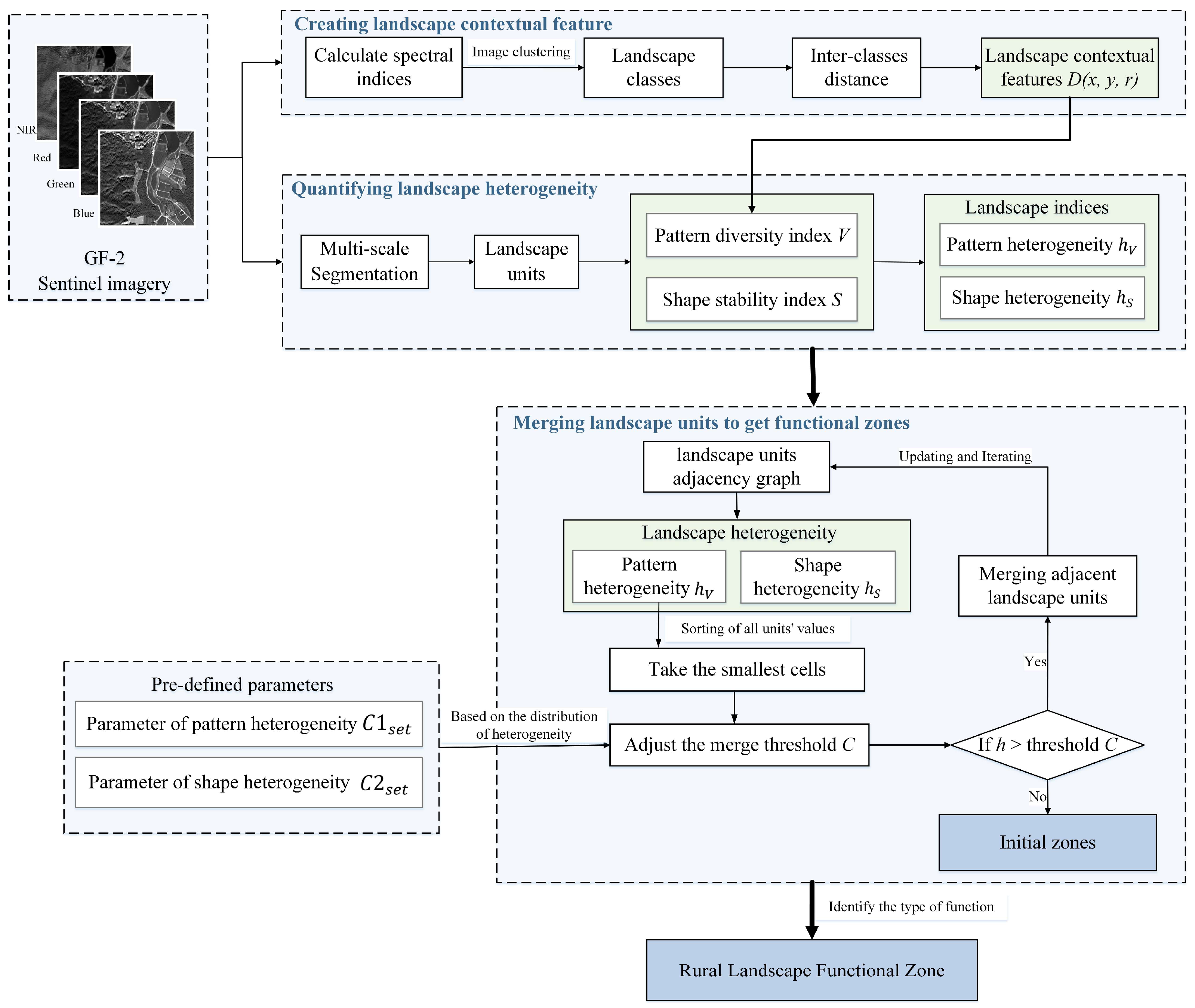
The methodology is shown in Figure 2. First, we calculated the spectral features and, then, clustered the imagery and constructed the contextual features of the landscape based on the distance between classes. Second, the image object obtained by the multiscale segment was used as the smallest landscape unit to calculate the landscape dominance index and shape index to quantity the landscape heterogeneity. Finally, according to the pre-defined parameters about the heterogeneity of the pattern and shape, the adjacent landscape units were automatically merged based on a rule to map boundaries for defining rural landscape functional zones. The map of the initial functional zone boundary was automatically generated in this process, and the final functional zones of an area were obtained according to the landscape type and the main functions in the zones.

2.3. Landscape Contextual Features

In rural and peri-urban regions, land use planning is primarily concerned with the management of regional land cover and landscapes [10]. The analysis of landscape patterns is critical to understanding landscape functions [49], and land use is a fundamental data source that is often used to quantitatively analyze landscape patterns and, thus, characterize landscape functions [50]. Therefore, this study proposes landscape contextual features based on land cover types as a basis for mapping the boundaries of functional zones. This approach quantitatively measures the characteristics of rural landscape patterns by considering the spatial distribution of different landscape cover types. The main steps in the calculation of this indicator included the classification of landscape cover and the measurement of the spatial characteristics of landscape cover types.

2.3.1. Landscape Classification

Remote sensing image clustering is a common tool for land cover analysis currently [50]. The rural landscape in rural regions of Southwestern China is predominantly comprised of woodlands, farmlands, and water areas. To fully utilize the spectral information of remote sensing imagery, three spectral indices (Table 2) were used to be stacked with the original four-band imagery to create dimensional feature maps. After standardizing the feature maps, landscape clustering was performed by the K-means clustering algorithm. The clustering came out as r groups of landscape cover classes.

2.3.2. Landscape Contextual Features

The geographically closest distance between different image classes has been considered a fundamental basis for functional zone classification [51]. Spatial distance analysis between landscape cover classes is also commonly used in landscape spatial analysis [52]. Therefore, the spatial distribution characteristics among different landscape cover classes are utilized to measure the landscape pattern characteristics. This is usually achieved by calculating the geographic closest proximity of each pixel to different landscape cover types according to the distribution of r groups of landscape cover types [51]. When calculating the distance, the maximum distance value was limited to η to reduce the errors caused by the extreme values. The landscape contextual feature of each pixel represents the nearest distance d i of this pixel to the landscape cover type group i, which is a vector consisting of r elements. The landscape contextual feature vector can be expressed as:
D x , y , r = d 1 d 2 d i d r

2.4. Landscape Characteries

2.4.1. Landscape Units

Planning landscape functional zones is based on the characteristic differences of landscape units within a region [37]. In this study, the image objects obtained by multiscale segmentation were seeded as landscape units to measure the characteristics of the landscape. Here, the original multispectral imagery was segmented into spectrally homogeneous objects by multiresolution segmentation (MRS) in the eCognition9.0 software [53], and the optimum scale parameter of the segmentation was determined by an Estimation of Scale Parameter 2 (ESP2) tool [54]. Based on the landscape contextual feature vector in Section 2.3 the pattern diversity V of the landscape units was calculated based on the landscape dominance. The landscape dominance measures the extent to which the landscape is controlled by several major landscape types, with a larger value indicating greater differences in the proportion of each landscape cover class in the landscape unit [55]. It is a useful metric for evaluating the composition characteristics and differences of regional landscape diversity. The pattern diversity V is calculated as follows:
V = [   l n ( a ) + P i ln P i ]
where a denotes the area of the landscape unit and P i is the proportion of the grid feature value d i in the ith dimension to the sum of all (number r) dimensional landscape grid feature values in a certain landscape cover type, with a value range of (0~1).
In addition, the shape stability is proposed based on the patch shape index [56]. A value of the shape stability closer to zero indicates that the shape of the landscape unit is closer to a circle, which is more conducive to efficient operation and management within the unit. When a denotes the area of the landscape unit and l denotes the perimeter of the landscape unit, the shape stability S of the landscape unit can be calculated from the formula below:
S = | 1 l 2 π × a |

2.4.2. Landscape Heterogeneity Indices

Landscape heterogeneity is the basis for functional zone mapping, and it usually includes compositional and conformational heterogeneity [43]. In this study, the heterogeneity characteristics of the landscape were measured based on the pattern diversity and shape stability. A landscape unit adjacency map was first constructed based on the spatial distribution of the landscape units. Then, the changes in the characteristics of landscape heterogeneity before and after merging the two adjacent landscape units were calculated. Finally, pattern heterogeneity and shape heterogeneity can be used as the basis for judging whether to merge landscape units or not. Pattern heterogeneity indicates the compositional characteristics of landscape units in terms of the number and spatial distance, and shape heterogeneity shows the shape variation of the landscape units. The area and pattern diversity of two adjacent landscape units are represented by a 1 , a 2 and V 1 , V 2 respectively. The area and pattern diversity of the merged target are represented by a m e r g and V m e r g . The pattern heterogeneity index h V is defined as:
h V = V m e r g ( V 1 × a 1 + V 2 × a 2 ) / a m e r g
The area and shape stability of two adjacent landscape units are denoted by a 1 , a 2 and S 1 , S 2 , respectively, and the area and shape stability of the merged target are denoted by a m r e g and S m e r g . The shape heterogeneity index h S can be obtained as follows:
h S = S m e r g ( S 1 × a 1 + S 2 × a 2 ) / a m e r g

2.5. Automatic Definition of Boundaries

When mapping landscape functional zones, the application of computer automation techniques to evaluate landscape feature differences is an emerging trend [57,58]. This study proposes an automatic approach to defining functional zone boundaries. The landscape heterogeneity indices used for merging judgment include pattern heterogeneity and shape heterogeneity. If the value of landscape heterogeneity values is below the merging threshold, the two adjacent landscape units will merge into the same landscape functional zone. In the process of mapping, as the area of a landscape unit increases, the distance from its pixels to other units and cover classes also increases. This results in a higher overall value of landscape contextual features for the units. To address the errors in contextual features caused by the area of the landscape unit, we propose a method to automatically adjust the merging threshold C according to the distribution of background features in the landscape unit. The merging threshold is defined as:
C = C s e t × d ¯ i , j d ¯ m ,               i f ( d ¯ i > d u q & d ¯ j > d u q ) C s e t ,                                             o t h e r w i s e
The merging thresholds contain the pattern heterogeneity threshold and the shape heterogeneity threshold denoted by C 1 and C 2 . The value of C s e t is to be determined artificially in advance, including C 1 s e t and C 2 s e t . The values of d ¯ i and d ¯ j represent the mean values of the landscape contextual feature values of all pixels in the current landscape units i and j , respectively, while d ¯ i , j represents the mean value of the merged landscape units. The values of d ¯ m and d u q are the median and upper quartile of the distribution of the mean values of the landscape contextual features for all landscape units. This means that the only parameters that require user input in each automated mapping process are C 1 s e t and C 2 s e t , representing the landscape indices’ thresholds.
During the automatic drawing, the h V of all landscape units are sorted, and the unit with the smallest h V is given priority in judging whether to merge. If both h V and h S are below the zoning thresholds of C 1 and C 2 , respectively, the units are merged to create a new landscape unit. The adjacency map and the landscape heterogeneity are updated before continuing the loop. The process iterates until the zoning parameter criteria cannot be satisfied, at which point, the boundary distribution map for rural landscape functional zones is output.

2.6. Evaluation of Mapping Quality (Reference Functional Zone Boundary)

Traditionally, existing zoning data and open social data [59] can be the basis for validating the results in urban functional zones, but this is rare in most rural regions [42]. In this study, the boundaries of reference zones are manually delineated referring to existing planning data, investigating information and visual interpretation by high-resolution imagery from GF-2. When sketching the reference functional zones, we focused on the functions of ecological services, agricultural production, and human living in the rural regions. The reference boundaries were obtained according to the type, size, and spatial distance of land use in the rural regions. In order to quantify the spatial relationship between the mapped functional zones and the reference functional zones, we calculated the matching rate (MR) and inclusion ratio (IR). Finally, the recall and precision accuracy of each functional zone type (TRA and TPA) and the overall accuracy of the functional zone type (OA) were used to quantify the accuracy of the method in mapping different types of functional zones, which can be calculated based on Table 3.

3. Result

The results are presented in two parts. First, we conducted experiments using the method in Case A to show the results of each step, to analyze the images of the preset parameters on the final mapping results and to determine the best way to set the parameters. Then, in order to verify the feasibility and applicability of the method in rural areas with different grid types, we applied the same method and analyzed the results in Case B and Case C.

3.1. Results of the Experimental Validation in Case A

3.1.1. Metrics of Landscape Characteristics

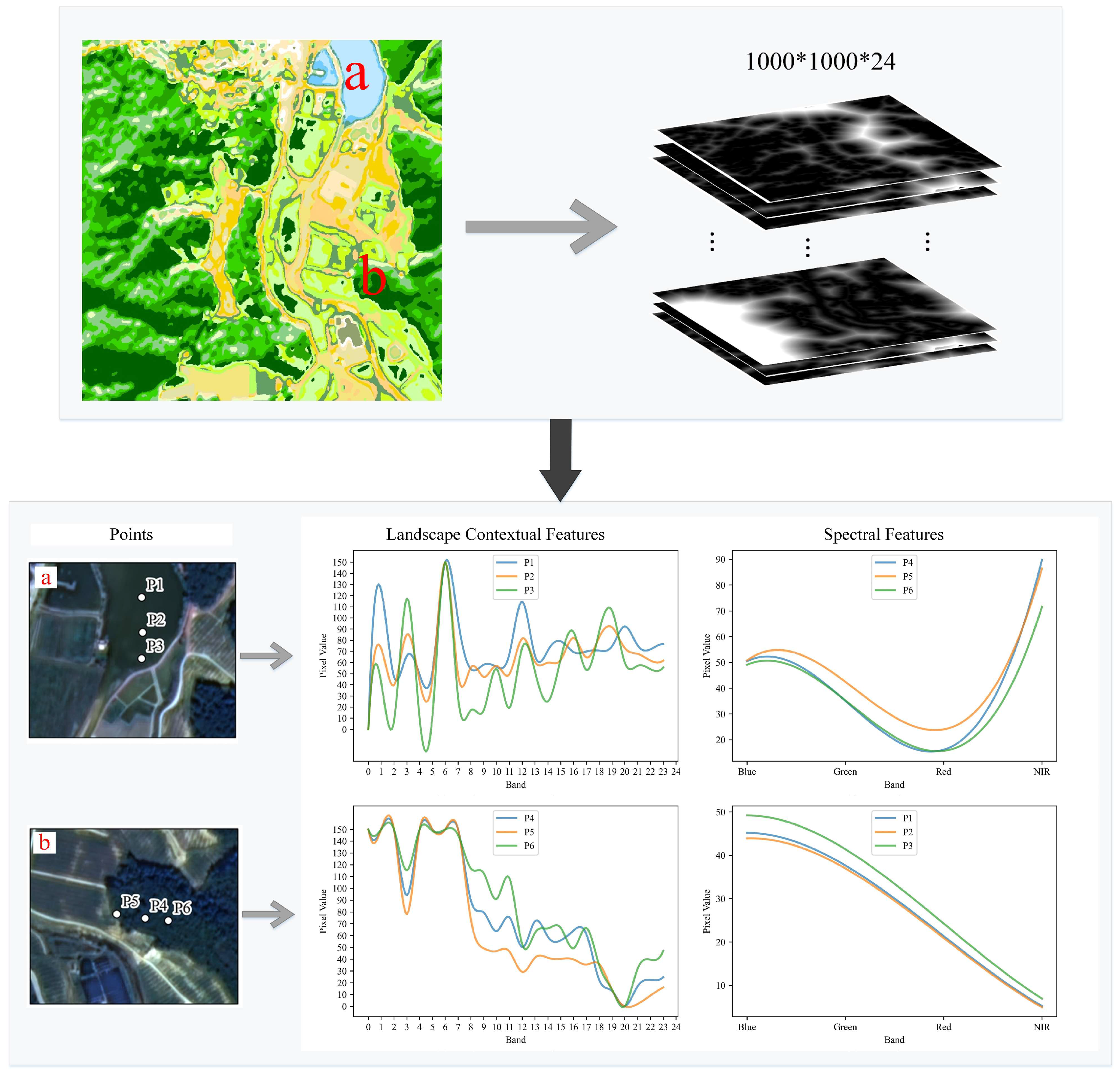
As shown in Figure 3, K-means image clustering was performed in the ENVI5.3 software to classify pixels into 24 classes according to landscape cover in Case A. Then, the distances between classes were calculated to obtain a map of landscape contextual features (shape: 1000 × 1000 × 24). Figure 3 shows the curve features of the spectral and landscape contextual features for points in two different landscape cover types. It shows that the general trend in the distribution of spectral and landscape context features was the same for different points within the same landscape cover type. However, the latter values became smaller with increasing distance from the boundary location, which can represent spatial distance information. Figure 4 shows the 94 image objects obtained by MRS, and the scale parameter was 135 in the eCognition9.0 software. This also means 94 landscape units were regarded as the smallest units in Case A, and then, a regional adjacency map was constructed from the landscape units. Based on the adjacency map, a total of 217 initial landscape heterogeneity arrays were calculated in Case A, and the numerical distribution of the pattern heterogeneity and shape heterogeneity is shown in Figure 4c.

3.1.2. Impact of the Pre-Defined Parameters of Pattern Heterogeneity

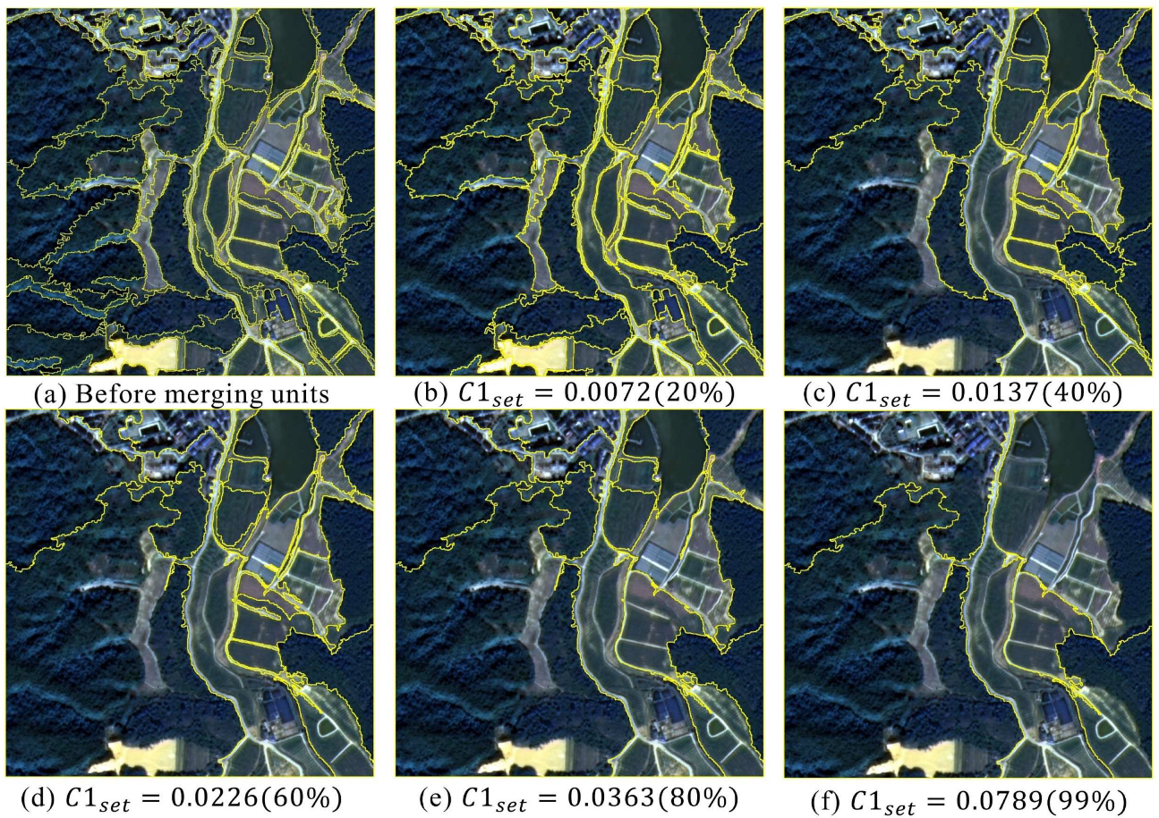
The C 1 s e t was determined by selecting the percentile distribution of the pattern heterogeneity value h V of all landscape units before merging. C 2 s e t was fixed at 0.1 in Case A, and then, five parameter values were set for mapping according to a 20% step. The resulting functional zone boundary maps (Figure 5) were compared with visually interpreted maps. Figure 5 shows that the number of functional zones decreased significantly with increasing experimental values of C 1 s e t . When C 1 s e t was too small, the boundary distribution was disorganized, but when C 1 s e t was set too large, there was no obvious main landscape type in the zone. By setting C 1 s e t between the 60th and 99th percentile of h V , the areas of agricultural land, buildings, forest land, water, and other types, aggregated landscape elements were divided into different landscape functional zones. It can be inferred that the optimal parameters exist within this percentile range.
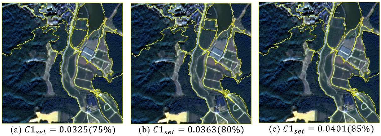
To identify the optimal parameters within a certain percentage range, we conducted experiments using a 5% incremental approach. Specifically, we used locally weighted regression (LWR) to fit curves depicting the relationship between the number of functional zones, the mean value of pattern diversity, and the mean value of shape stability with changes in C 1 s e t , and the curves are named loess fitting curves (refer to Figure 6). As shown in Figure 6, an increase in C 1 s e t led to a decrease in the number of functional zones and a smaller mean value of shape stability, while the mean value of pattern diversity increased correspondingly. Notably, there was a stable range between the C 1 s e t values of the 70th to 90th percentile, representing the optimal parameter range. To delineate the functional zone boundary, we took the 75th, 80th, and 85th percentile values of h V within the stable variation curve as the values for C 1 s e t . The visual comparison analysis in Figure 7 shows that the best state occurred when a value of 0.0401 (85th percentile of h V ) was chosen.

3.1.3. Impact of the Pre-Defined Parameters of Shape Heterogeneity

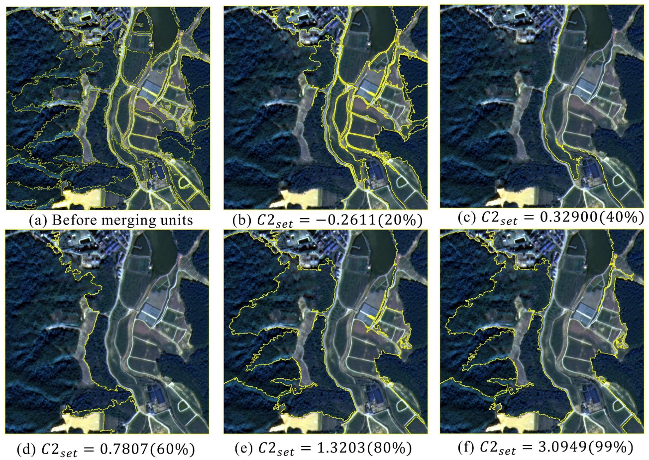
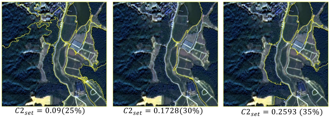
Similarly, to select a suitable value for C 2 s e t , we, according to Section 3.1.2, selected the value of C 1 s e t as 0.0401 in Case A. Then, five merging parameters based on the 20% increment for the percentile of the shape heterogeneity value of h S were selected before the merged unit. We visually interpreted and compared the functional zoning results (refer to Figure 8) and found that no regular changes in the functional zone boundary occurred when C 2 s e t was greater than 0.32900 (the 40th percentile of h S ). When C 2 s e t was −0.2611, we were able to distinguish the areas of each concentrated landscape element type, but the boundaries of the agricultural landscape areas were too finely divided. We inferred that the optimal parameter range lay between the 20th and 40th percentile. Since this range was small, we tested the parameter values in 5% increments within this percentile range. The functional zone boundaries obtained from this test are shown in Figure 8.
From Figure 9, we confirmed that the optimal parameter range was between the 20th and 30th percentile because there was no clearly dominant landscape element type within the functional zone when C 2 s e t was greater than the 30th percentile. Since the boundary distribution varied greatly with C 2 s e t , we conducted another test within the 20th to 30th percentile range. The loess curve in Figure 6 shows that an increase in C 2 s e t resulted in a decrease in the number of functional zones, a smaller mean value of the shape stability value, and a larger mean value of the pattern diversity. However, when C 2 s e t was at the 25th, 26th, and 27th percentile of h S , the plotted boundary results were consistent, which enabled us to more reasonably aggregate the same land types while ensuring the area had certain diversity characteristics and a simpler shape. Therefore, we concluded that the 25th, 26th, and 27th percentiles of h S were more-suitable merging scale parameters for C 2 s e t .

3.1.4. The Final Rural Landscape Functional Zones

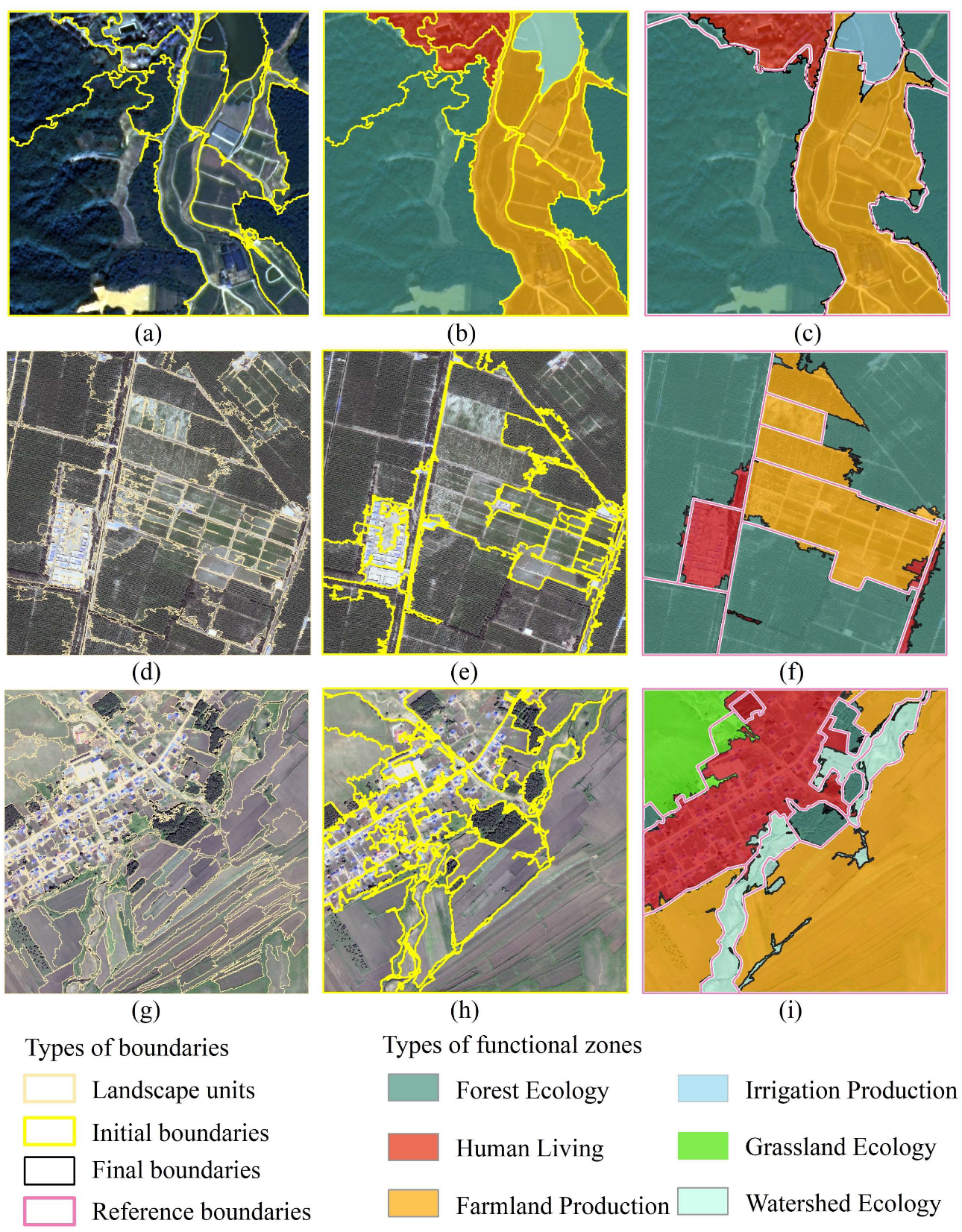
After analyzing the effects of different parameters on the effect of automatically merging units in Section 3.1.2 and Section 3.1.3, we determined the best parameters for Case A: C 1 s e t = 0.0401 (85th percentile of h V ) and C 2 s e t = 0.00987 (26th percentile of h S ). After merging the neighboring landscape units that met the threshold conditions, 14 initial rural landscape functional zones were obtained from 95 landscape units (Figure 10a). The initial zones were spatially evaluated as shown in Table 4, and although the MR values were low, the initial zones had a high inclusion rate, indicating that most of the initial functional zones were within the range of the reference functional zones.
After conducting a visual interpretation of the high-resolution images, we were able to define the type of each initial functional zone based on the major landscape elements present within that area (refer to Figure 10b). There were four types of functional zones in Case A: (1) rural forest ecological functional zone, which is dominated by forests and mainly performs ecological functions; (2) rural living functional zone, which is dominated by residential buildings and meets the living needs of rural residents; (3) rural farmland production functional zone, mainly farmland, to meet the needs of efficient and intensive agricultural production; (4) rural irrigation production functional zone, with ponds and ditches as the main part, giving full play to the role of agricultural irrigation in the water. To enhance the efficiency of intensive resource management, we merged adjacent initial functional zones with the same function into optimized landscape functional zones. The spatial boundaries of these optimized functional zones, along with the reference functional zones, are depicted in Figure 10c.
As shown in Table 4, the high values of MR and IR between the mapped functional zones and the reference functional zones indicate a strong alignment in boundary morphology, and there was no lack of merging or over-merging. The evaluation of the zoning method for Case A, as shown in the confusion matrix in Table 5, demonstrated promising results. The overall accuracy achieved by this method was 95.9%, indicating high accuracy and consistency. The accuracy of the results for all types of functional zones was notably improved, suggesting a favorable outcome.

3.2. Application of Different Rural Pattern Types

Following the procedure in Section 2.3, the preprocessed imagery underwent image clustering to calculate the landscape contextual features. The resulting features were then quantified based on image objects. For Case B and Case C, multiple pixels were segmented into 95 and 141 landscape units, respectively (shown in Figure 10d,g). The parameter analysis method discussed in Section 3.1.2 and Section 3.1.3 was employed to select the following parameters for the two cases:
  • For Case B, C 1 s e t = 0.0746 (80th percentile of h V ), and C 2 s e t = 0.0009 (25th percentile of h S ).
  • For Case C, C 1 s e t = 0.0596 (90th percentile of h V ), and C 2 s e t = 0.0284 (23rd percentile of h S ).
After applying the automated mapping method outlined in Section 2.5, we successfully generated 25 initial zones for Case B (depicted in Figure 10d) and 39 initial zones for Case C (shown in Figure 10g). Our methodology effectively combined numerous small, heterogeneous units to form larger, relatively homogeneous functional zones. As shown in Table 4, the MRs of the initial functional regions of Case B and Case C were both much smaller than the IRs, and their IRs were both greater than 80%, implying that most of their initial functional zones were also included in the areas of the reference functional zones.
When defining the type of each initial functional, Case B was identified as three types of initial rural functional zones: forest ecological functional zone, living functional zone, and farmland production functional zone; these types were also defined based on the major landscape elements present within the area. The initial zone of Case C was classified into two more types than Case B: (1) rural grassland ecological functional zone, which is dominated by grassland and mainly performs ecological functions; (2) rural watershed ecological functional zone, which is around a river and performs ecological functions. To obtain the final functional zones, we manually merged the initial functional zones with the same landscape cover type that were adjacent to each other, based on the primary landscape cover type within each initial functional zone. Figure 10f,i display the final functional zones along with the reference boundaries for Case B and Case C, respectively. Table 4 shows that the values of MR and IR for the final zones in Case B and Case C were all bigger than 80%, and comparing the final boundaries with the reference boundaries revealed a significant spatial overlap between them.
In Table 5, the results of Case B demonstrated an overall accuracy (OA) of 89.0%, indicating a favorable overall outcome. Specifically, it achieved improved accuracy in distinguishing between living areas and other zone types, as well as effectively grouping contiguous areas of tree plantations within the same zone. However, challenges were encountered in accurately differentiating between crop areas and areas with intercropped trees. In Case C, the results presented in Table 5 showed an overall accuracy (OA) of 92.1%, indicating a high level of accuracy. This method proved effective in accurately delineating large concentrated crop and grassland areas, as well as successfully separating the river bank area from adjacent farmland. It should be noted that Case C includes a greater diversity of zone types and a larger number of initial landscape units compared to Case B. However, there was a lower accuracy (TRA) observed when mapping the watershed functional zones. This can be attributed to the smaller size of the river and the absence of distinctive boundaries in the area. Additionally, the method demonstrated lower positional accuracy (TPA) when mapping forested zones within the prairie zones, likely due to the smaller size of the forests and their susceptibility to merging with neighboring building zones. These findings suggested the need for further investigation and adjustment of the method to improve accuracy in these specific areas.

4. Discussion

4.1. Ability to Quantify Landscape Characteristics

Quantifying the function in a region is a complex work for functional zoning in rural regions. In our study, we extracted the landscape contextual features and constructed landscape pattern heterogeneity and landscape shape heterogeneity in an object-oriented method for quantifying differences in rural functions. Rural landscapes are an amalgamation of natural ecological structures and anthropogenic landforms built by humans based on natural landscapes [60], and the landscape patterns are distinctive in different places. As shown in Figure 3, landscape context features provide additional distance information along with the spectral features, which is critical for spatial planning. The construction of landscape contextual features based on spectra remedies the weaknesses of the aforementioned spectral features. It makes use of the category information represented by the reflectance of the features and can also represent the spatial distance information of the categories, all of which echo the information needs of the functional zoning of the landscape. As for quantitative indices, landscape pattern heterogeneity and landscape shape heterogeneity do well in quantifying the size, type, shape, and spatial combination of landscape units, which are important landscape structural features in landscape zoning. Moreover, the multiscale segmentation generates arbitrary-scale units with the lowest heterogeneity according to feature information, which takes into account the characteristics of the aggregation and fragmentation of the rural feature distribution and avoids the “pretzel” phenomenon [32], and the object-oriented approach also effectively solves the problem of the poor performance of K-means clustering when considering both the spatial dimensions and spatial relationships of landscape zoning [61]. Our study demonstrated that a combination of landscape heterogeneity and image segmentation methods for quantifying rural function is preferable for mapping geographic boundaries.

4.2. A Multiscale Merging of Units to Obtain Functional Zones

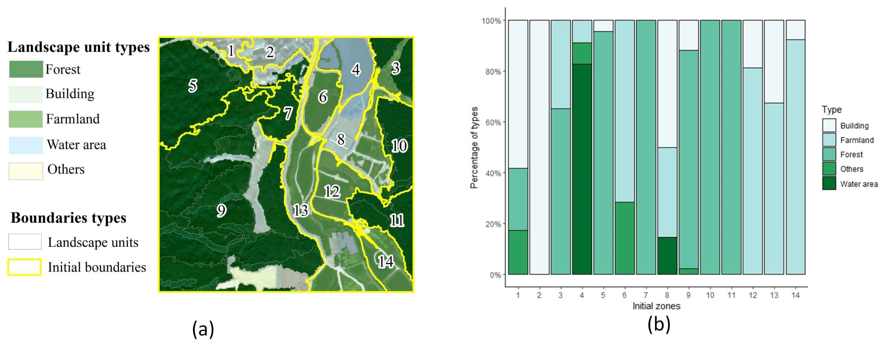
A multiscale merging method was proposed to automatically map rural landscape functional zones from the smallest landscape units. It takes into account not only the inherent characteristics of the units themselves, but also the overall heterogeneity, making full use of the unit information to obtain the optimal parameters. As depicted in Figure 11, the automated mapping results successfully separated different landscape types within the region, leading to the creation of functional zones that are diverse and contain distinct landscape subjects. These zones were divided into different functional zones based on the type and proportion of each landscape type within the zone. For instance, Zone 1 and Zone 2 are both building living zones, but Zone 1 exhibits a higher abundance of trees and other land types (as shown in Figure 11b). Consequently, in the automatic mapping process, they were treated as two separate functional zones. Although the initial functional zones generally had a low MR, they had a high IR due to their small scale, and they were generally surrounded by the reference functional zones. From the perspective of scale conversion, functional zones at this scale facilitate a finer measure of the distribution of functional zones in a village and can also be used to plan functional zones at a larger scale. The final boundaries and types of the functional zone are determined by adjusting according to the main landscape type and spatial adjacencies.

4.3. Applicability to Functional Zoning in Villages with Different Landscape Patterns

Mapping functional zones is critical for effective planning and management of an area. Each region has its own unique characteristics, requiring different factors and methods for mapping and identifying areas. The landscape pattern characteristics of rural areas are closely tied to the geographical features of the region, and understanding the differences in landscape patterns between regions is crucial for rural planning and management. In this paper, an M2LHI method was proposed, and three rural areas with typical landscape pattern characteristics in China were selected for testing. The method combines terrain and landscape types and utilizes remote sensing satellite images, which provide comprehensive and detailed monitoring of rural areas. It utilizes sophisticated image segmentation techniques to process complex images and utilizes the high efficiency of computers for automatic analysis and execution. Additionally, it incorporates classical landscape zoning theory to achieve functional zoning of rural areas with diverse landscape pattern characteristics. The proposed method offers a scientific analysis of landscape patterns and enables the combination and arrangement of different landscape units. It also allows for semi-automatic mapping to delineate boundaries of regional functional zones. The M2LHI method minimizes the influence of human subjective factors while providing convenience for rural area managers and planners. Moreover, rural is only a relative concept to urban in many studies [48], so it can be validated in future studies by applying it after categorizing different rural areas according to some information, such as local climatic zones [8], precinct ventilation zones, the heat island effect, etc.

4.4. Limitation

Although the M2LHI methodology demonstrated its utility and efficiency in automatically mapping the boundaries of functional zones in different rural areas, there are still several areas for future improvement. The match and inclusion rates for the initial and final zones in each case were above 78%, except for the initial zone with a match rate below 40%. This indicates that the M2LHI method selected the optimal parameters to obtain the initial functional zone, and it was accurate in determining the location of the function; however, further merging of the initial zone is required to align it with the reference functional zone in terms of spatial scope. The result will be affected by the input parameters C 1 s e t and C 2 s e t , and different parameters may affect the final accuracy. Automatic drawing of the boundaries can divide human life, production, and the ecological environment in rural areas into different zones, but there are fuzzy boundaries and irregular shapes of functional zones, which also reduce the matching rate and the overall accuracy of mapping final functional zones with different functions. The transition area from one type of feature over to another, where there is little difference in pixel values, leads to fuzzy boundaries, which is a problem that also existed in previous studies [47]. Although both landscape contextual features and shape features were considered in the landscape unit-merging process, it underperformed in dealing with narrow landscape units, which is because a functional zone would contain different types of land cover. In fact, the boundaries of the functional zones are drawn based on the automatic merging of the landscape units, so their shape and position may be determined by the image objects obtained from segmentation. While obtaining landscape units through the MRS of the eCongniton software is fast and easy to operate, future improvements should focus on enhancing the segmentation algorithm to generate landscape units with simpler and more-regular shapes, which can serve as the foundation for mapping functional zone boundaries.
In addition, the M2LHI method made it difficult to distinguish between crop and tree areas in the results of Case B. This challenge arose because both crops and young forests are vegetation and are hard to differentiate solely based on the spectral characteristics utilized in this study. In Case C, fragmented stands may be incorrectly combined with surrounding areas into one functional zone, but it is very important to independently differentiate tree plantation areas for ecological evaluation in grassland regions. Therefore, in the future, strongly relevant data sources should be added based on the village characteristics to help map management boundaries. For example, local industrial planning data, road distribution, and terrain height data could be added as data sources to improve the rationality of mapping functional zones. In future research, the application should be validated in images of larger area sizes and the methodology should be improved based on the results to provide accurate functional zone results for mapping rural landscapes in areas of different sizes.

5. Conclusions

Reasonable functional zone boundaries for rural landscapes play an important role in the sustainable use of natural resources and the prosperous development of society and the economy. To meet the rural landscape management needs of rural areas in the technological era, this study presented the M2LHI method for mapping the rural landscapes functional zones based on VHR satellite imagery. Using GF-2 satellite images as the data source, the method was applied to three rural landscapes in China with different typical landscape pattern characteristics for validation, and we obtained the following conclusions.
(1) China’s Gaofen-2 (GF-2) satellite imagery is able to provide sufficient information for rural landscape zoning. Constructing landscape contextual features combined with an object-oriented approach can successfully quantify landscape heterogeneity and construct geomorphic units of rural regions with different landscape pattern types.
(2) Merging the smallest landscape units based on landscape heterogeneity can realize the leap from homogeneous landscape units to rural landscape functional zones.
(3) The M2LHI method is applicable to rural regions with different landscape pattern characteristics and is capable of mapping functional zones with high accuracy and stability.
In summary, the proposed M2LHI method can simultaneously utilize remote sensing technology and the automatic execution capability of computers based on classical landscape functional zoning theories. This study lays a solid scientific groundwork for rural landscape management and development planning in such regions. For future research, the inclusion of additional data sources or exploring alternative multiscale segmentation methods could potentially enrich the landscape feature set and enhance the overall scientific validity of the study.

6. Patents

The work reported in this manuscript resulted in a patent named “A method and system for functional zoning of rural landscapes based on scale adaptation” (Patent Number CN202210521176.6).

Author Contributions

Y.Z.: conceptualization, methodology, validation, formal analysis, data curation, writing—original draft preparation, visualization. Y.D.: conceptualization, methodology, validation, resources, writing—review and editing, supervision, project administration. Z.G.: validation, writing—review and editing. C.Y.: conceptualization, methodology, writing—review and editing, visualization. X.W.: methodology, visualization. All authors have read and agreed to the published version of the manuscript.

Funding

This research was funded by the National Key Research and Development Program of China (Grant Number 2019YFD1100401) and the Project of Fundamental Research Funds for the Central Universities (2662023YLPY003).

Data Availability Statement

The data that support the findings of this study are available from the corresponding author, Y.D., upon reasonable request.

Acknowledgments

It is acknowledged that the GF-2 imagery data were acquired from the Hubei Centre for Resources Satellite Data and Application website at “https://logindataservices.ceode.ac.cn/cas/login?service=http://ids.ceode.ac.cn/gfds/gflogin” (accessed on 9 December 2021).

Conflicts of Interest

The authors declare no conflict of interest.

References

  1. Liu, H.; Jiang, G.; Zhuang, H.; Wang, K. Distribution, utilization structure and potential of biomass resources in rural China: With special references of crop residues. Renew. Sustain. Energy Rev. 2008, 12, 1402–1418. [Google Scholar] [CrossRef]
  2. Zhang, L.; Luo, Z.; Mallon, D.; Li, C.; Jiang, Z. Biodiversity conservation status in China’s growing protected areas. Biol. Conserv. 2017, 210, 89–100. [Google Scholar] [CrossRef]
  3. Picuno, P.; Cillis, G.; Statuto, D. Investigating the time evolution of a rural landscape: How historical maps may provide environmental information when processed using a GIS. Ecol. Eng. 2019, 139, 105580. [Google Scholar] [CrossRef]
  4. Yang, Y.; Bao, W.; Liu, Y. Coupling coordination analysis of rural production-living-ecological space in the Beijing-Tianjin-Hebei region. Ecol. Indic. 2020, 117, 106512. [Google Scholar] [CrossRef]
  5. Wang, C.; Tang, N. Spatiotemporal characteristics and evolution of rural production living- ecological space function coupling coordination in Chongqing Municipality. Geogr. Res. 2018, 37, 1100–1114. [Google Scholar]
  6. Tan, X.L.; An, Y.; Su, Y.; Zhou, G.; He, Y. Spatio-temporal Dynamics of Agricultural Function in Changsha-Zhuzhou-Xiangtan Urban Agglomerations. Sci. Geogr. Sin. 2018, 38, 708–716. [Google Scholar]
  7. He, B.-J.; Ding, L.; Prasad, D. Enhancing urban ventilation performance through the development of precinct ventilation zones: A case study based on the Greater Sydney, Australia. Sustain. Cities Soc. 2019, 47, 101472. [Google Scholar] [CrossRef]
  8. Liu, H.; He, B.-J.; Gao, S.; Zhan, Q.; Yang, C. Influence of non-urban reference delineation on trend estimate of surface urban heat island intensity: A comparison of seven methods. Remote. Sens. Environ. 2023, 296, 113735. [Google Scholar] [CrossRef]
  9. Locke, C.M.; Rissman, A.R. Factors influencing zoning ordinance adoption in rural and exurban townships. Landsc. Urban Plan. 2015, 134, 167–176. [Google Scholar] [CrossRef]
  10. Liu, Y.; Fu, B.; Zhao, W.; Wang, S.; Deng, Y. A solution to the conflicts of multiple planning boundaries: Landscape functional zoning in a resource-based city in China. Habitat Int. 2018, 77, 43–55. [Google Scholar] [CrossRef]
  11. Fan, J. Draft of major function oriented zoning of China. Acta Geogr. Sin. 2015, 70, 186–201. [Google Scholar]
  12. Nie, W.; Yang, F.; Xu, B.; Bao, Z.; Shi, Y.; Liu, B.; Wu, R.; Lin, W. Spatiotemporal Evolution of Landscape Patterns and Their Driving Forces Under Optimal Granularity and the Extent at the County and the Environmental Functional Regional Scales. Front. Ecol. Evol. 2022, 10, 954232. [Google Scholar] [CrossRef]
  13. Liu, Y.; Li, T.; Zhao, W.; Wang, S.; Fu, B. Landscape functional zoning at a county level based on ecosystem services bundle: Methods comparison and management indication. J. Environ. Manag. 2019, 249, 109315. [Google Scholar] [CrossRef]
  14. Zhang, B.; Zhong, C.; Gao, Q.; Shabrina, Z.; Tu, W. Delineating urban functional zones using mobile phone data: A case study of cross-boundary integration in Shenzhen-Dongguan-Huizhou area. Comput. Environ. Urban Syst. 2022, 98, 101872. [Google Scholar] [CrossRef]
  15. Newbold, T.; Hudson, L.N.; Hill, S.L.L.; Contu, S.; Lysenko, I.; Senior, R.A.; Börger, L.; Bennett, D.J.; Choimes, A.; Collen, B.; et al. Global effects of land use on local terrestrial biodiversity. Nature 2015, 520, 45. [Google Scholar] [CrossRef] [PubMed]
  16. Song, X.P.; Hansen, M.C.; Stehman, S.V.; Potapov, P.V.; Tyukavina, A.; Vermote, E.F.; Townshend, J.R. Global land change from 1982 to 2016. Nature 2018, 560, 639–643. [Google Scholar] [CrossRef]
  17. Usman, M.; Liedl, R.; Shahid, M.A.; Abbas, A. Land use/land cover classification and its change detection using multi-temporal MODIS NDVI data. J. Geogr. Sci. 2015, 25, 1479–1506. [Google Scholar] [CrossRef]
  18. Toure, S.I.; Stow, D.A.; Shih, H.-C.; Weeks, J.; Lopez-Carr, D. Land cover and land use change analysis using multi-spatial resolution data and object-based image analysis. Remote. Sens. Environ. 2018, 210, 259–268. [Google Scholar] [CrossRef]
  19. Tehrany, M.S.; Pradhan, B.; Jebuv, M.N. A comparative assessment between object and pixel-based classification approaches for land use/land cover mapping using SPOT 5 imagery. Geocarto Int. 2014, 29, 351–369. [Google Scholar] [CrossRef]
  20. Li, J.; Li, W.; Fu, J.; Gao, J.; Yang, L.; He, W. Using low-altitude UAV remote sensing to identify national park functional zoning boundary: A case study in Qianjiangyuan National Park pilot. Biodivers. Sci. 2019, 27, 42–50. [Google Scholar]
  21. Watmough, G.R.; Palm, C.A.; Sullivan, C. An operational framework for object-based land use classification of heterogeneous rural landscapes. Int. J. Appl. Earth Obs. Geoinf. 2017, 54, 134–144. [Google Scholar] [CrossRef]
  22. Zheng, X.; Wu, B.; Weston, M.V.; Zhang, J.; Gan, M.; Zhu, J.; Deng, J.; Wang, K.; Teng, L. Rural Settlement Subdivision by Using Landscape Metrics as Spatial Contextual Information. Remote. Sens. 2017, 9, 486. [Google Scholar] [CrossRef]
  23. Zhu, Y.; Liu, K.; Myint, S.; Du, Z.; Li, Y.; Cao, J.; Liu, L.; Wu, Z. Integration of GF2 Optical, GF3 SAR, and UAV Data for Estimating Aboveground Biomass of China’s Largest Artificially Planted Mangroves. Remote Sens. 2020, 12, 2039. [Google Scholar] [CrossRef]
  24. Ning, J.; Liu, J.; Kuang, W.; Xu, X.; Zhang, S.; Yan, C.; Li, R.; Wu, S.; Hu, Y.; Du, G.; et al. Spatiotemporal patterns and characteristics of land-use change in China during 2010–2015. J. Geogr. Sci. 2018, 28, 547–562. [Google Scholar] [CrossRef]
  25. Vadjunec, J.M.; Frazier, A.E.; Kedron, P.; Fagin, T.; Zhao, Y. A Land Systems Science Framework for Bridging Land System Architecture and Landscape Ecology: A Case Study from the Southern High Plains. Land 2018, 7, 27. [Google Scholar] [CrossRef]
  26. Kumar, D.; Shekhar, S. Statistical analysis of land surface temperature–vegetation indexes relationship through thermal remote sensing. Ecotoxicol. Environ. Saf. 2015, 121, 39–44. [Google Scholar] [CrossRef]
  27. Aslan, N.; Koc-San, D. The Use of Land Cover Indices for Rapid Surface Urban Heat Island Detection from Multi-Temporal Landsat Imageries. ISPRS Int. J. Geoinf. 2021, 10, 416. [Google Scholar] [CrossRef]
  28. Viana, C.M.; Girão, I.; Rocha, J. Long-Term Satellite Image Time-Series for Land Use/Land Cover Change Detection Using Refined Open Source Data in a Rural Region. Remote. Sens. 2019, 11, 1104. [Google Scholar] [CrossRef]
  29. Talukdar, S.; Singha, P.; Mahato, S.; Shahfahad; Pal, S.; Liou, Y.-A.; Rahman, A. Land-Use Land-Cover Classification by Machine Learning Classifiers for Satellite Observations—A Review. Remote. Sens. 2020, 12, 1135. [Google Scholar] [CrossRef]
  30. Radoux, J.; Defourny, P. A quantitative assessment of boundaries in automated forest stand delineation using very high resolution imagery. Remote. Sens. Environ. 2007, 110, 468–475. [Google Scholar] [CrossRef]
  31. Garcia-Pedrero, A.; Lillo-Saavedra, M.; Rodriguez-Esparragon, D.; Gonzalo-Martin, C. Deep Learning for Automatic Outlining Agricultural Parcels: Exploiting the Land Parcel Identification System. IEEE Access 2019, 7, 158223–158236. [Google Scholar] [CrossRef]
  32. Weidong, M.; Chunjing, L.; Zongming, W.; Mingming, J.; Dehua, M.; Mingyue, L.; Chunyan, L. Study on Dynamic of Wetlands Landscape in the Trans-boundary Regions between China and Russia of Ussuri River Watershed based on Object-oriented Classification Method. Remote Sens. Technol. Appl. 2016, 31, 378–387. [Google Scholar]
  33. Blaschke, T.; Hay, G.J.; Kelly, M.; Lang, S.; Hofmann, P.; Addink, E.; Feitosa, R.Q.; van der Meer, F.; van der Werff, H.; van Coillie, F.; et al. Geographic Object-Based Image Analysis—Towards a new paradigm. ISPRS J. Photogramm. Remote Sens. 2014, 87, 180–191. [Google Scholar] [CrossRef] [PubMed]
  34. Fernandes, M.R.; Aguiar, F.C.; Silva, J.M.; Ferreira, M.T.; Pereira, J.M. Optimal attributes for the object based detection of giant reed in riparian habitats: A comparative study between Airborne High Spatial Resolution and WorldView-2 imagery. Int. J. Appl. Earth Obs. Geoinf. 2014, 32, 79–91. [Google Scholar] [CrossRef]
  35. Wu, B.; Yu, B.; Shu, S.; Wu, Q.; Zhao, Y.; Wu, J. A spatiotemporal structural graph for characterizing land cover changes. Int. J. Geogr. Inf. Sci. 2021, 35, 397–425. [Google Scholar] [CrossRef]
  36. Aksoy, S.; Akcay, H.G.; Wassenaar, T. Automatic Mapping of Linear Woody Vegetation Features in Agricultural Landscapes Using Very High Resolution Imagery. IEEE Trans. Geosci. Remote. Sens. 2010, 48, 511–522. [Google Scholar] [CrossRef]
  37. Du, J.; Watts, J.D.; Jiang, L.; Lu, H.; Cheng, X.; Duguay, C.; Farina, M.; Qiu, Y.; Kim, Y.; Kimball, J.S.; et al. Context-Enabled Extraction of Large-Scale Urban Functional Zones from Very-High-Resolution Images: A Multiscale Segmentation Approach. Remote Sens. 2019, 11, 1952. [Google Scholar] [CrossRef]
  38. Li, C.; Liang, S.; Che, Q. Spatial Reconstruction of the Rural Settlements in Wuhu City Based on the Function Oriented Zoning. Resour. Environ. Yangtze Basin 2015, 24, 1736–1743. [Google Scholar]
  39. Moos, A.I.; Dear, M.J. Structuration Theory in Urban Analysis 1. Theoretical Exegesis. Environ. Plan. A 1986, 18, 231–252. [Google Scholar] [CrossRef]
  40. Zhang, X.; Du, S.; Wang, Q. Hierarchical semantic cognition for urban functional zones with VHR satellite images and POI data. ISPRS J. Photogramm. Remote. Sens. 2017, 132, 170–184. [Google Scholar] [CrossRef]
  41. Yohannes, H.; Soromessa, T.; Argaw, M.; Dewan, A. Changes in landscape composition and configuration in the Beressa watershed, Blue Nile basin of Ethiopian Highlands: Historical and future exploration. Heliyon 2020, 6, e04859. [Google Scholar] [CrossRef]
  42. Du, S.H.; Du, S.; Liu, B.; Zhang, X. Mapping large-scale and fine-grained urban functional zones from VHR images using a multi-scale semantic segmentation network and object based approach. Remote Sens. Environ. 2021, 261, 12480. [Google Scholar] [CrossRef]
  43. Fahrig, L.; Baudry, J.; Brotons, L.; Burel, F.G.; Crist, T.O.; Fuller, R.J.; Sirami, C.; Siriwardena, G.M.; Martin, J.-L. Functional landscape heterogeneity and animal biodiversity in agricultural landscapes. Ecol. Lett. 2011, 14, 101–112. [Google Scholar] [CrossRef]
  44. Xiao, J.; Watanabe, T.; Lu, X.; Chand, M.B.; Umarhadi, D.A.; Chen, X.; Avtar, R. Integrating land use/land cover change with change in functional zones’ boundary of the East Dongting Lake National Nature Reserve, China. Phys. Chem. Earth 2022, 126, 103041. [Google Scholar] [CrossRef]
  45. Nielsen, M.M.; Ahlqvist, O. Classification of different urban categories corresponding to the strategic spatial level of urban planning and management using a SPOT4 scene. J. Spat. Sci. 2015, 60, 99–117. [Google Scholar] [CrossRef]
  46. Du, S.H.; Du, S.; Liu, B.; Zhang, X.; Zheng, Z. Large-scale urban functional zone mapping by integrating remote sensing images and open social data. Giscience Remote Sens. 2020, 57, 411–430. [Google Scholar] [CrossRef]
  47. Zheng, Z.; Du, S.; Du, S.; Zhang, X. A multiscale approach to delineate dune-field landscape patches. Remote. Sens. Environ. 2020, 237, 111591. [Google Scholar] [CrossRef]
  48. Stewart, I.D.; Oke, T.R. Local Climate Zones for Urban Temperature Studies. Bull. Am. Meteorol. Soc. 2012, 93, 1879–1900. [Google Scholar] [CrossRef]
  49. Willemen, L.; Liu, Y.; Lü, Y.-H.; Feng, X.-M. Landscape pattern analysis in landscape ecology: Current, challenges and future. Acta Ecol. Sin. 2008, 28, 5521–5531. [Google Scholar]
  50. Verburg, P.H.; Hein, L.; van Mensvoort, M.E. Spatial characterization of landscape functions. Landsc. Urban Plan. 2008, 88, 34–43. [Google Scholar] [CrossRef]
  51. Nielsen, M.M. Remote sensing for urban planning and management: The use of window-independent context segmentation to extract urban features in Stockholm. Comput. Environ. Urban Syst. 2015, 52, 1–9. [Google Scholar] [CrossRef]
  52. Chen, W.; Xiao, D.; Li, X. The Characteristics and Contents of Landscape Spatial Analysis. Acta Ecol. Sin. 2002, 22, 1135–1142. [Google Scholar]
  53. Hay, G.J.; Castilla, G.; Wulder, M.A.; Ruiz, J.R. An automated object-based approach for the multiscale image segmentation of forest scenes. Int. J. Appl. Earth Obs. Geoinf. 2005, 7, 339–359. [Google Scholar] [CrossRef]
  54. Drăguţ, L.; Csillik, O.; Eisank, C.; Tiede, D. Automated parameterisation for multi-scale image segmentation on multiple layers. ISPRS J. Photogramm. Remote Sens. 2014, 88, 119–127. [Google Scholar] [CrossRef]
  55. Chao, W.; Ai, G.; Du, L.; Yan, L. Analysis of Landscape Ecological Effects before and after the Land Consolidation Take Land Consolidation Project in Liuxuanyao Villige in Zezhou County in Shanxi Province. J. Shanxi Agric. Sci. 2010, 38, 49–52. [Google Scholar]
  56. Yao, W.; Zhang, Y.; Zhu, Q. Effects of woodland spatial distribution on soil erosion in small watershed: A case study in Wuqi County, Northern Shaanxi. Sci. Soil Water Conserv. 2015, 13, 16–22. [Google Scholar]
  57. Jellema, A.; Stobbelaar, D.-J.; Groot, J.C.; Rossing, W.A. Landscape character assessment using region growing techniques in geographical information systems. J. Environ. Manag. 2009, 90, S161–S174. [Google Scholar] [CrossRef]
  58. Zhang, H.; Wang, Y.; Shang, J.; Liu, M.; Li, Q. Investigating the impact of classification features and classifiers on crop mapping performance in heterogeneous agricultural landscapes. Int. J. Appl. Earth Obs. Geoinf. 2021, 102, 102388. [Google Scholar] [CrossRef]
  59. Zhang, X.; Du, S.; Wang, Q.; Zhou, W. Multiscale Geoscene Segmentation for Extracting Urban Functional Zones from VHR Satellite Images. Remote. Sens. 2018, 10, 281. [Google Scholar] [CrossRef]
  60. Liu, L.; Li, Z.; Zhang, H. Discussion on characteristics of Chinese rural landscape and its planning objectives and contents. Ecol. Environ. 2004, 13, 445–448. [Google Scholar]
  61. Liu, Y.; Zhou, Y.; Li, Y. Rural regional system and rural revitalization strategy in China. Acta Geogr. Sin. 2019, 74, 2511–2528. [Google Scholar]
Figure 1. Location of the study areas in China. (Case A is located in Fujian Province and represents hilly countryside. Case B is located in Xinjiang Province and represents flat countryside. Case C is situated in the Inner Mongolia Autonomous Region and represents grassland countryside.)
Remotesensing 15 04920 g001
Figure 2. Methodology for mapping rural landscape functional zones.
Remotesensing 15 04920 g002
Figure 3. Construction of landscape contextual features. The upper section shows the shape and origin of the contextual features, and the bottom section shows the landscape context features and spectral feature for area a in water and area b in forest.
Remotesensing 15 04920 g003
Figure 4. Metrics of landscape characteristics: (a) remote sensing objects obtained by multiscale segmentation, and each unique color represents each individual object; (b) landscape units, and every object has its own number as an identifying label for subsequent calculations; (c) histogram of landscape heterogeneity features.
Remotesensing 15 04920 g004
Figure 5. The effect of different values of C 1 s e t on the automatic merging.
Remotesensing 15 04920 g005
Figure 6. Loess fitting curves for landscape unit characteristics at different values.
Remotesensing 15 04920 g006
Figure 7. Influence of different values of C 1 s e t on the actual zoning results within the steady state of the change in landscape unit characteristics.
Remotesensing 15 04920 g007
Figure 8. Effects of different values of C 2 s e t on automatic merging (step is 20%).
Remotesensing 15 04920 g008
Figure 9. Effects of different values of C 2 s e t on zoning merging (step is 5%).
Remotesensing 15 04920 g009
Figure 10. Mapping results. (a) shows 14 initial functional zones obtained from merging units; (b) shows the types of initial functional zones; (c) is a comparison of the final mapping boundaries and reference boundaries. In Case B and Case C: (d,g) are the smaller landscape units in Case B and Case C; (e,h) show the initial zones; (f,i) demonstrate the functional types of zones, the reference functional zones, and final functional zones.
Remotesensing 15 04920 g010
Figure 11. Multiscale heterogeneous initial functional zones. (a) The distribution of landscape units with different types. (b) The area proportion of different landscape unit types in initial functional zones.
Remotesensing 15 04920 g011
Table 1. Specific information on the three study areas.
CaseLocation ProvincePatternsMain Landscape Cover Types
Case AFujianHilly countrysideOpen low-rise, dense trees, low plants, water
Case BXinjiangFlat countrysideLarge low-rise, dense trees, low plants
Case CInner Mongolia Autonomous RegionGrassland countrysideSparsely built, dense trees, low plants, water
Notes: Main landscape cover types are defined according to abridged definitions for local climate zones [48].
Table 2. Spectral indices and calculation formulas.
IndexIndex Full NameEquations
NDVINormalized Difference Vegetation Index N I R R e d N I R + R e d
SAVISoil-Adjusted Vegetation Index N I R R e d ( N I R + R e d + L ) × ( 1 + L )
NDWINormalized Difference Water Index G r e e n N I R G r e e n + N I R
Notes: NIR, Red, and Green represent the spectral bands. The parameter L varies with vegetation density, taking values between 0 and 1. When vegetation cover is high, L = 0.
Table 3. Metrics used for evaluating mapping qualities.
Evaluation MetricsEquationsExplanations
Matching ratio
(MR)
M R = Z r Z m Z r / N r A bigger value signifies a better match.
Inclusion ratio
(IR)
I R = Z r Z m Z m / N m A value of one indicates the whole mapping zone is within the reference zone, and a bigger value indicates a better match.
Recall accuracy of each functional zone type (TRA) T R A = T m r T r Represents the proportion of accurately mapped area that aligns with the reference functional zone type.
Precision accuracy of each functional zone type (TPA) T P A = T m r T m Measures the accuracy of defining the actual functional zone type, represented as a percentage of correctly classified area.
Overall accuracy
(OA)
O A = T m r T r Indicates the overall accuracy of mapping functional zones with different functions.
Notes: where Z r is the area of a polygon in reference zones, Z m is the area of the corresponding polygon in the mapping zones, and Z r Z m represents the overlapped area. N r and N m mean the number of reference zones and mapping zones, respectively. As for different types of functional zones, T r and T m indicate the area of one type of reference functional zone and mapping zone, respectively, and T m r means the area of the final functional zone where the functional type can be correctly defined.
Table 4. Estimation of the spatial relationship of mapping result.
Case AMR (%)IR (%)Case BMR (%)IR (%)Case CMR (%)IR (%)
Initial zones39.994.0Initial zones28.181.1Initial zones27.583.8
Final zones93.178.5Final zones81.180.7Final zones89.285.5
Table 5. Mapping accuracy of rural landscape functional zones with different functions.
Case AOA: 95.9%ForestFarmlandBuildingIrrigation
TRA (%)96.795.194.792.0
TPA (%)98.0095.583.389.4
Case BOA: 89.0%ForestFarmlandBuilding
TRA (%)99.167.065.4
TPA (%)87.195.894.1
Case COA: 92.1%ForestFarmlandBuildingGrasslandWatershed
TRA (%)98.691.486.967.389.5
TPA (%)93.091.396.490.979.0
(Forest: rural forest ecology functional zone; Farmland: rural farmland production functional zone; Building: rural building living functional zone; Irrigation: rural irrigation production functional zone; Grassland: rural grassland ecology functional zone; Watershed: rural watershed ecology functional zone).
Disclaimer/Publisher’s Note: The statements, opinions and data contained in all publications are solely those of the individual author(s) and contributor(s) and not of MDPI and/or the editor(s). MDPI and/or the editor(s) disclaim responsibility for any injury to people or property resulting from any ideas, methods, instructions or products referred to in the content.