Article

A Study of the Method for Retrieving the Vegetation Index from FY-3D MERSI-II Data

1
National Climate Center, Chinese Meteorological Administration, Beijing 100081, China
2
Operation and Administration Center for River Basin Hydro Complex, China Three Gorges Corporation, Yichang 443133, China
*
Author to whom correspondence should be addressed.
Remote Sens. 2023, 15(2), 491; https://doi.org/10.3390/rs15020491
Submission received: 26 November 2022 / Revised: 5 January 2023 / Accepted: 6 January 2023 / Published: 13 January 2023

Abstract

:
NDVI data have been widely used to detect and monitor vegetation status at regional, continental, and global scales. FY-3D MERSI-II NDVI (FNDVI) is a critical operational product used in many studies monitoring ecosystems and agriculture and assessing climate change and its risks, including drought and fire. MERSI-II and MODIS have very similar spectral response functions in the red and near-infrared channels, making MERSI/NDVI an effective replacement for MODIS/NDVI (MNDVI). Therefore, it is critical to conduct a thorough evaluation of the product’s quality. In this study, the consistency characteristics of two normalized difference vegetation index (NDVI) products, FY-3D MERSI-II NDVI and MODIS NDVI, were compared and validated at national and regional scales in China from 2020 to 2021. To assess the consistency of these two NDVI datasets, the correlation coefficient, root-mean-square error, and mean bias error were used. The findings revealed that the spatial distribution patterns of FNDVI and MNDVI were highly consistent across the country at the monthly time scale. The correlation coefficients were greater than 0.9475 for the two years 2020–2021, while the average deviation was between 0.02 and 0.05, and the root-mean-square error was 0.11. Based on the difference in the time consistency between FNDVI and MNDVI, the changes in the monthly NDVI values of the two types of satellites are generally consistent across the country. Among the three typical experimental areas, the relative deviation of the regional time series for products was the highest in Xinjiang. The relative average deviation of FNDVI in other regions was low, and its change trend was consistent with that of MODIS.

1. Introduction

Vegetation is the most important land cover on the terrestrial surface, and it is sensitive to global change. Vegetation plays an important role in the earth’s system and affects the earth’s energy balance. It is the key sensitive indicator for the impact of humans and climate on the environment so that the current situation and the evolution of vegetation growth can be predicted quickly and accurately [1,2]. The vegetation index is a method used for the detection of satellite data. It can reflect the growth status of green vegetation to estimate the characteristics of the conditional distribution [3].
Remote-sensing instruments record the portions of the electromagnetic spectrum that are not absorbed by the atmosphere by measuring the electromagnetic radiation reflected and emitted from the terrestrial surface. Methodologies for monitoring vegetation change in response to various climatic fluctuations have been developed using remote-sensing technology. The normalized difference vegetation index (NDVI) is one such methodology. It is a remote system for vegetation monitoring at both temporal and spatial scales, and it is based on the differential reflection properties of green vegetation in the visible and infrared portions of the spectrum [4,5]. NDVI data have been widely used to detect and monitor vegetation status at regional, continental, and global scales. Many studies have shown that the NDVI is proportional to the fraction of absorbed photosynthetically active radiation, leaf area, vegetation fraction, and net primary productivity. Thus, it can be used to assess vegetation conditions [6,7,8]. Presently, a sufficient number of studies have successfully used this technique to analyze and characterize vegetation in different regions [9,10,11]. The NDVI has already been successfully used to study temporal and spatial trends and variations in vegetation distribution, productivity, and dynamics to monitor habitat loss and fragmentation and the ecological effects of climate disasters such as drought. The NDVI has become an extremely useful tool for terrestrial ecologists intending to better understand how vegetation dynamics and distributions affect diversity and life history traits and the human impact on the environment [12]. The NDVI is one of the most important indicators for the qualitative and quantitative assessment of vegetation growth. The evaluation of the consistency between NDVI products obtained by different sensors is conducive to a better understanding of the long-term effects of environmental and climate change [13].
China’s first-generation polar-orbiting meteorological satellite, FY-1A, was launched in 1998, followed by the FY-1B and FY-1C satellites [14,15]. FY-3 satellites can obtain global, all-weather, three-dimensional, quantitative, and multispectral characteristic parameters of the atmosphere and the terrestrial and marine surfaces [16,17], which have been widely used in China and around the world in weather forecasting and climate, ecological environment, and disaster monitoring and have remarkable economic and social benefits [18]. FY-3D, China’s second-generation polar-orbiting meteorological satellite, was launched on 15 November 2017. FY-3D is the fourth operational satellite in the FY-3 series. It is equipped with ten remote-sensing instruments, including the newly developed infrared hyperspectral atmospheric sounder, hyperspectral greenhouse gas monitor, wide-angle auroral imager, and ionosphere photometer. FY-3D’s orbit altitude, inclination, quasi-repeat time, and ascending node local time are 831 km, 98.753°, 4–10 days, and 14:00, respectively [19]. MERSI is the primary visible infrared optical imaging remote-sensing instrument aboard China’s second-generation polar-orbiting meteorological satellite, which is expected to carry an improved medium-resolution spectral imager [20]. Every day, it can obtain global 250 m resolution true-color images and images of two infrared split windows with no gaps. It is considered one of the most advanced wide-range imaging remote-sensing instruments in the world [21,22], and the MERSI NDVI is also a key operational product on the FY3D satellite [23].
Terra and Aqua are a series of satellites in the Earth Observing System (EOS) program in the United States. Both satellites are equipped with the Moderate Resolution Imaging Spectrometer (MODIS), which has 36 bands (0.405~14.385 µm); the spatial resolution of bands 1–2 is 250 m, and the spatial resolution of bands 3–7 is 500 m, while the spatial resolution of bands 8–36 is 1000 m, and the scanning width is 2330 km. MODIS can be used for the long-term global observation of the Erath’s surface, biosphere, atmosphere, and ocean [24,25,26]. The MODIS vegetation index (VI) products were specially designed to monitor terrestrial photosynthetic activity and provide more consistent spatial and temporal comparisons of global vegetation conditions. FY-3D and MODIS are currently the most widely used sensors.
Evaluating the difference between FY-3D and the MODIS NDVI sensor is of great significance for the consistency of NDVI data. This study aimed to develop a practical algorithm with improved input parameters in support of generating NDVI products from FY-3D MERSI-II data. The cross-validation of the MODIS-derived NDVI products, compared to the current FY-3D MERSI-II operational NDVI (FONDVI) generated from the ground operational system, an operational system through which FY series satellite products and data are produced and distributed to operational departments for application, improved the accuracy of the FY3D vegetation index through the reconstruction and establishment algorithms and determined the reasons for the difference in the NDVI. Therefore, these products can contribute to climate change, the ecological environment, agriculture, and other fields to promote better data-sharing services and international cooperation projects.

2. Materials and the Study Area

2.1. The FY-3D/MERSI-II Data

MERSI II, the next-generation polar-orbiting meteorological satellite, was built on the development and enhancement of MERSI I sensor technology. It was designed for weather forecasting, climate change monitoring, and earth environmental monitoring. The primary goal was to develop a three-dimensional atmospheric detection system and significantly improve the global data acquisition system as well as to improve cloud and surface characteristics remote sensing and obtain global, all-weather, three-dimensional, quantitative, multispectral data on atmospheric, land surface, and sea surface characteristic parameters [27]. The MERSI II sensor has 25 spectral channels, including 6 visible, 10 visible/near-infrared, 3 short-wave infrared, and 6 medium/long-wave infrared spectral channels. On the basis of the type I instrument, one visible spectral channel was removed, and five infrared spectral detection channels and one 1.38 µm channel were added to the short-wave infrared cirrus detection channel; the original central wavelength of the 11.25 µm spectral channel was changed to the central wavelengths of 10.8 µm and 12 µm. The MERSI II ground resolutions were 250 m (6 bands) and 1000 m (19 bands) (Table 1).
The 250 m high-resolution image provides the means for identifying, extracting, and analyzing more detailed features such as land surface, sea surface, and clouds [28]. FY-3D data can be obtained from the National Satellite Meteorological Centre of China (http://satellite.nsmc.org.cn/PortalSite/Data/DataView.aspx?currentculture=zh-CN, accessed on 1 March 2022). Scholars have used FY3/MERSI data to conduct research monitoring vegetation growth and the distribution of vegetation types, the spatial distribution and dynamic evolution of drought characteristics, the dynamic monitoring and assessment of flood and waterlogging disasters, and water quality monitoring [29,30]. Several solar reflection channels were optimized and adjusted, and 1.38 µm was added to the short-wave infrared cirrus detection channel. To obtain calibration accuracy indices of 5% in the visible and near-infrared band and 0.5 K in the infrared channel, the type II instrument has made great progress in the design of its visible on-board scaler, on-board blackbody, and solar-stray shielding [31]. At the same time, by increasing the cold-air detection angle and adding a special lunar observation mode, we can enhance the lunar observation ability and realize on-orbit lunar calibration [32,33]. The test data were the observation data of FY-3D MERSI-II NDVI. The data were stored as grid data, with resampling at a spatial resolution of 0.05 ° and a monthly time scale, adopting an equal longitude and latitude projection covering China and its surrounding areas with longitude and latitude ranges of 18°–54°N and 73°–135°E, respectively. The valid NDVI values were within the ranges of—2000~10,000 [34].

2.2. The MODIS Data

The main principles for selecting research data were as follows: (1) image data with fewer clouds and aerosols were selected to avoid masking ground information and more accurately retrieve the surface reflectance and (2) the transit time of imaging sensor data for comparison was as consistent as possible to avoid changes in the atmospheric conditions, solar altitude angle, and solar azimuth angle caused by the differences in transit time.
EOS/MODIS data, obtained from the website of the NASA Data Archive Center (http://ladsew.nascom.nasa.gov, accessed on 1 January 2022), provided level-1B 1 km MOD02 and 1 km MYD02 data products and their corresponding MOD03 and MYD03 geographic coordinate products. Since the comparison parameter used in this study, the band of the NDVI, is the visible red band (0.6–0.7 µm) that strongly absorbs green plants, along with the near-infrared band with high reflectance and high transmission to green plants (0.7–1.1 µm), the first and second bands of EOS/MODIS and the third and fourth bands of FY-3D/MERSI were selected in this study.
The MODIS data used in this study were from the MOD13A2 product acquired from Aqua MODIS. The MOD13A2 product included the 16-day composite NDVI with a 1 km resolution and data quality assurance (QA). The MODIS data correction included corrections for the effects of atmospheric gases (water vapor and ozone) and aerosols [35]. The external inspection data were the Aqua/MODIS MYD13C2 product. The data consisted of global grid data with equal longitude and latitude, a spatial resolution of 0.01 degrees, a monthly time scale, and an effective value between—2000 and 10,000. MODIS images were collected across China from February 2020 to December 2021. Because the two NDVI datasets had different time ranges, we chose the intersection of the three periods from February 2020 to December 2021 to conduct the research. Referring to the MOD13A2 monthly dataset’s synthesis method, the monthly NDVI values allowed for a comparison of their consistency. Moreover, the MOD13A3 NDVI and the FY3D NDVI products were resampled to the resolution of the MODIS NDVI (5 km) to satisfy the spatial correspondence of the surface features in the two NDVI datasets.

2.3. The Study Region

China is located in the east of Eurasia, along the west coast of the Pacific Ocean, and it is the world’s third largest country, with a territory area of 9.6 million km2 lying between latitudes 18° and 54°N and between longitudes 73° and 135°E. The landscape is generally characterized by major mountain ranges on the western side, high plateaus in the north, and low-relief regions in the east. Most of its rivers generally flow to the east. Broad grasslands predominate on the edges of the Inner Mongolian Plateau in the north, while Southern China is dominated by hills and low mountain ranges. To the east, extensive alluvial plains along the shores of the Yellow and East China Seas are dedicated to intensive farming activities. Across China, the terrain gradually descends from east to west. The Qinghai Tibet Plateau, known as “the roof of the world,” is the largest and highest plateau, with an average elevation of more than 4000 m. Mount Qomolangma, the highest peak in the world, is located on the plateau and is the main Himalayan peak. The climate is regionally variable, reflecting the country’s complex topography, and is primarily characterized by dry seasons and wet monsoons. The rainfall generally decreases from the southeast to the northwest. China’s land-use classes mainly include six categories of forest, farmland, grassland, city and town, bare land and desert, and water body (Figure 1). The vegetation regions mainly include forest, farmland, grassland, and desert.

3. Methodology

3.1. The Framework for NDVI-Specific Bias Correction

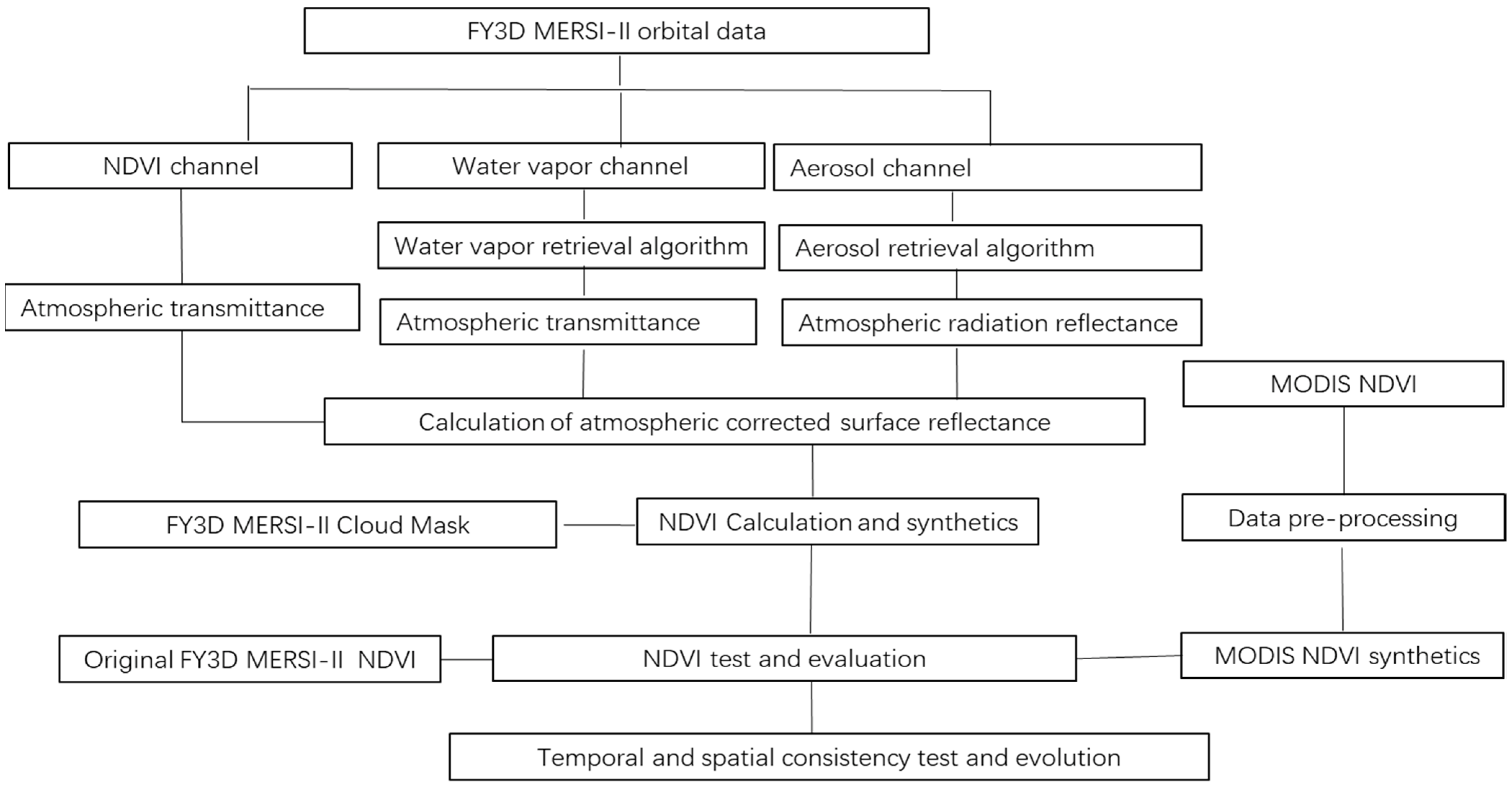
The technical framework for bias correction based on the NDVI with the L1 original radiation data was developed, and the technical route is illustrated as follows: (1) the Fy-3D/MERSI-II orbital data preprocessing steps included HDF data analysis, radiation calculation, band data extraction, angle data extraction, etc.; (2) atmospheric aerosol retrieval from the MERSI data was performed based on the black target algorithm; (3) the atmospheric transmittance, atmospheric scattering reflectance, and atmospheric spherical albedo were calculated; (4) the surface reflectance was obtained using an atmospheric correction of the orbital data; (5) The calculation of the NDVI with surface reflectance was tracked; (6) the 16-day and monthly NDVI products were synthesized; and (7) the FY3D-NDVI was validated. A flow chart is shown in Figure 2.

3.2. Atmospheric Molecular Transmittance

The atmospheric transmittance of the first four reflection bands of MERSI can be approximately considered as the ozone transmittance,   T O μ s , μ v ; atmospheric water vapor transmittance, T H μ s , μ v   ; and molecular atmospheric transmittance, consisting of the atmospheric downward radiation transmittance,   T R   μ s , and uplink radiation transmittance, T R   μ v ). The calculation formula of ozone transmittance, T O μ s , μ v , is as follows:
T O μ s , μ v = e x p [ 1 μ s + 1 μ v × U × A ]
In the above formula, U is the total mass of ozone in the atmosphere, which was considered to be 0.319 cm in this study, and A is the absorption coefficient of the ozone, which can be retrieved from studies of atmospheric transmittance [36].
The atmospheric water vapor transmittance,   T H μ s , μ v   , was calculated as follows:
T H μ s , μ v = e x p e x p A H + B H l n 1 μ s U H + 1 μ v U H
In the above formula,   U H is the content of atmospheric water vapor, which was taken as 2.93 g/cm2, and A H and B H . are water vapor absorption coefficients, as observed in Table 2.
Scattered atmospheric molecules are not absorbed, and the asymmetry factor is 0. The atmospheric downward radiation transmittance,   T R   μ s   , and the uplink radiation transmittance, T R   μ v   , can be obtained using the following formula:
T R μ s = 2 3 μ s 2 3 μ s e τ / μ s 4 3 + μ s
T R μ v = 2 3 μ v 2 3 μ v e τ / μ v 4 3 + μ v

3.3. Atmospheric Molecular Scattering

Atmospheric molecular scattering is also called Rayleigh scattering ( ρ R μ s , μ v , φ ). Its calculation requires the sum of the single-scattering and multiple-scattering contributions [37]. Its specific calculation formula is as follows:
ρ R μ s , μ v , φ = m = 0 2 2 δ 0 , m × ρ l m μ s , μ v , τ × cos m φ + 1 e τ / μ s × 1 e τ / μ v × m = 0 2 2 δ 0 , m × Δ m τ × P m μ s , μ v × c o s m φ
In the above formula, τ refers to the optical thickness of the atmospheric molecules scattered from the target surface in the corresponding band (Table 3), which is consistent with the atmospheric pressure (P) of the target area, and the optical thickness of the atmospheric molecules in this band ( τ 0 ) under standard atmospheric pressure ( P 0 ) was calculated using the 6S radiative transfer mode by inputting the spectral response function of the corresponding band of the MERSI sensor; δ 0 , m is Kronecker function; and P m μ s , μ v is the mth value of the scattering phase function of the atmospheric molecules after the Fourier expansion.
The calculation formula of the first three terms is Equation (3); ρ l m   μ s , μ v , τ represents the single-scattering reflectance corresponding to the scattering phase function of the item M, and its calculation formula is shown in Equation (9); Δ m τ is the correction term of multiple scattering corresponding to the optical thickness of the atmospheric molecules. The calculation formulas of the first three terms are as follows:
P 0 µ s , µ v = 1 + 3 µ s 2 1 3 µ v 2 1 × 1 δ 2 δ 1 + 2 δ 2 δ × 1 8
P 1 µ s , µ v = µ s µ v 1 µ s 2 1 2 1 µ v 2 1 2 × 1 δ 2 δ 1 + 2 δ 2 δ × β × 1.5
          P 2 µ s , µ v = 1 μ s 2 1 μ v 2 × 1 δ 2 δ 1 + 2 δ 2 δ × β × 0.375
where   δ = 0.0279 , β = 0.5
ρ l m µ s , µ v , τ = P m µ s , µ v × 1 e τ 1 μ s + 1 μ v × 1 4 µ s + µ v Δ m τ = a m + b m × l n τ
In the above formula, when m = 0 the calculation formulas of a 0 and b 0 are as follows:
a 0 = a 0 0 + a 1 0 µ s µ v + a 2 0 µ s µ v 2 + a 3 0 µ s + µ v + a 4 0 µ s 2 + µ v 2
b 0 = b 0 0 + b 1 0 µ s µ v + b 2 0 µ s µ v 2 + b 3 0 µ s + µ v + b 4 0 µ s 2 + µ v 2
In the above formula, the a 0 0 , a 1 0 , a 2 0 , a 3 0 , and a 4 0 values were 0.332438, –0.103244, 0.162854, 0.114933, and –0.309248, respectively; the b 0 0 , b 1 0 , b 2 0 , b 3 0 , and b 4 0 values were –0.067771, 0.032417, 0.001577, –0.035037, and –0.012409, respectively. When m was considered to be 1 and 2, the corresponding values of a 1 ,   a 2 ,   b 1 , and b 2 were 0.19666, 0.145459, –0.054391, and –0.029108, respectively.

3.4. The Dark Target Aerosol Inversion Algorithm

In reference to the MODIS dark target aerosol retrieval algorithm [38], this study developed a dark target aerosol remote-sensing retrieval algorithm for MERSI data by retrieving the aerosol optical thickness and aerosol type for the MERSI land area. The algorithm considers the point where the 2.12 um band of the land surface dark target pixel has a certain linear relationship with the surface reflectance in the 0.66 um and 0.47 um channels. The formula is as follows:
ρ 0.66 s = f ( ρ 2.12 s ) = ρ 2.12 s × s l o p e 0.66 / 2.12 + y i n t 0.66 / 2.12
ρ 0.47 s = g ( ρ 0.66 s ) = ρ 0.66 s × s l o p e 0.47 / 0.66 + y i n t 0.47 / 0.66
Relevant variables in the above formula are defined as follows:
s l o p e 0.66 / 2.12 = s l o p e 0.66 / 2.12 n d v i s w i r + 0.002 0.27
y i n t 0.66 / 2.12 = 0.00025 + 0.033
s l o p e 0.47 / 0.66 = 0.49
y i n t 0.47 / 0.66 = 0.005
and
s l o p e 0.66 / 2.12 n d v i s w i r = 0.48 ;   n d v i s w i r < 0.25
  s l o p e 0.66 / 2.12 n d v i s w i r = 0.58 ;   n d v i s w i r > 0.75
s l o p e 0.66 / 2.12 n d v i s w i r = 0.48 + 0.2 n d v i s w i r 0.25 ; 0.25 n d v i s w i r 0.75
The specific methods used were as follows:
First, through the accurate atmospheric correction based on the observation data obtained from ground-based stations, the statistical relationship of the spectral surface reflectance ratio with the short-wave infrared and visible bands was determined, which was used as prior knowledge for the reflectance estimation of the decoupling of ground air. Second, the radiative transfer model’s lookup table was used to interpolate and calculate the simulated reflectivity of the top layer of the atmosphere with different aerosol optical thickness values at the same observation angle for each aerosol type. To complete the aerosol parameter inversion procedure, the aerosol optical thickness with the smallest error value and the corresponding aerosol type were determined by calculating the angle between the simulated reflectivity and the apparent reflectance observed by the satellite.

3.5. Atmospheric Correction Algorithm

The purpose of atmospheric correction is to eliminate the influences of (1) the atmosphere and light on the reflection from the ground object and obtain formal physical model parameters such as the reflectivity, emissivity, and surface temperature of the ground object; (2) atmospheric water vapor, oxygen, carbon dioxide, methane, and ozone on the reflection from the ground object; and (3) the atmospheric molecules and aerosol scattering. In this study, the purpose of the atmospheric correction was mainly to eliminate the effects of atmospheric molecular absorption, atmospheric molecular scattering, and aerosol absorption and scattering in the reflectance data from MERSI-II L1 orbital observations and obtain the main calculation steps of the surface reflectance. The specific formula is as follows:
ρ T O A θ S , θ v , s v = T g O 3 , O 2 , C O 2 , m ρ R + ( ρ 0 ρ R ) T g H 2 O ( M ,   U H 2 O 2 + T θ S T θ V ρ s 1 S ρ s T g H 2 O M , U H 2 O
In the above formula, ρ T O A is the observed reflectance of the top layer of the atmosphere, which is the value observed for the L1 data after radiation correction; ρ R is the Rayleigh scattering reflectance, which can be calculated using Formula (5); and ρ 0 is the sum of the Rayleigh-scattering and aerosol-scattering reflectance, which was mainly calculated using the aerosol optical thickness, aerosol type, and air pressure. The lookup table (LUT) was precalculated in this study using the 6S radiative transfer code [39]. ρ S   is the surface reflectance and the final result of atmospheric correction; S is the atmospheric spherical reflectance, which was obtained through the previous LUT synchronous query and interpolation; T   θ s / v represents the upward and downward atmospheric transmittance caused by aerosol and molecular scattering, respectively, and it was obtained through the previous LUT synchronous query and interpolation; and Tg is the atmospheric transmittance due to the absorption of gas molecules, which can be calculated using Formulas (1)–(4).

3.6. The Calculation of NDVI

The contrast between reflectance in the near-infrared band and that in the infrared band is a sensitive index for vegetation measurements. The canopy vegetation index is the spectral transformation of infrared and near-infrared reflectance, and its value is between –1 and +1. It is usually expressed as follows:
N D V I T O A = ρ N I R T O A ρ R E D T O A ρ N I R T O A + ρ R E D T O A
In the above formula, ρ refers to the surface reflectance after atmospheric correction. ρ N I R T O A and ρ R E D T O A represent the near-infrared and red-light bands, respectively.
The orbital data can be divided into daily NDVI products or the 16-day synthetic products generated from daily NDVI products, and multi-phase data can be synthesized. In the synthesis process, the overlapping area in the multi-period data is involved. This study used the constraint view angle maximum value composite (CVMVC). This algorithm avoids the error caused by the large observation angle of the maximum value compositing (MVC) algorithm. At the same time, this algorithm is more stable and reliable than the BRDF algorithm, with fewer computation steps, and it is also suitable for long-term business operations. The algorithm’s processing flow is to collect NDVI and multi-observation-angle data pixel by pixel in the overlapping area, select high-quality NDVI data, sort by small/large zenith angle observations, and finally retain the larger value from the first two NDVI values. The zenith angle observation is also written into the auxiliary file at the same time.

3.7. Validation

In this work, after the time and space matching of data, the MODIS NDVI product was used as the inspection source to conduct a quantitative quality inspection of the data and a comparative analysis of the MERSI NDVI. The deviation (BIAS), root-mean-square error (RMSE), and correlation coefficient (CORR) indicators were selected and used to evaluate the accuracy of satellite-based remote-sensing products [40,41]. The calculation method of these statistical scores can be demonstrated as follows:
B i a s = | x i x o i |
R S M E = 1 N i = 1 N X i X o i 2
C o r r = i = 1 N X i X ¯ X o i X o ¯ i = 1 N X i X ¯ 2 i = 1 N X o i X o ¯ 2
where X i represent the FNDVI data, X o represents the MNDVI; X ¯ is the average of FNDVIs, X o ¯ is the average of MNDVIs; and N is the amount of valid NDVI input data. Bias represents the difference between the FY-3D monthly NDVI value and the MODIS NDVI value, which can reflect the standard deviation of NDVI values each month. The correlation coefficient was used to determine the linear relationship between the variables at a fixed distance. The RMSE was used to measure the deviation of the observed value from the true/actual value, and it is very sensitive to large or small errors in group measurements. Therefore, the RMSE can effectively reflect the precision of measurement.

4. Results

4.1. Spatial Distribution Assessment Quality

The deviation correction method was used to process the FY3D/MERSI data for FNDVI products. To compare them with the MODIS and FONDVI products, we resampled the FNDVI products in space, where the resolution was consistent with that of the MODIS and FONDVI products. The spatial distribution assessment of quality, test of time consistency, and test of typical regional time-series consistency were carried out for the FNDVI products to evaluate their effect of deviation correction.
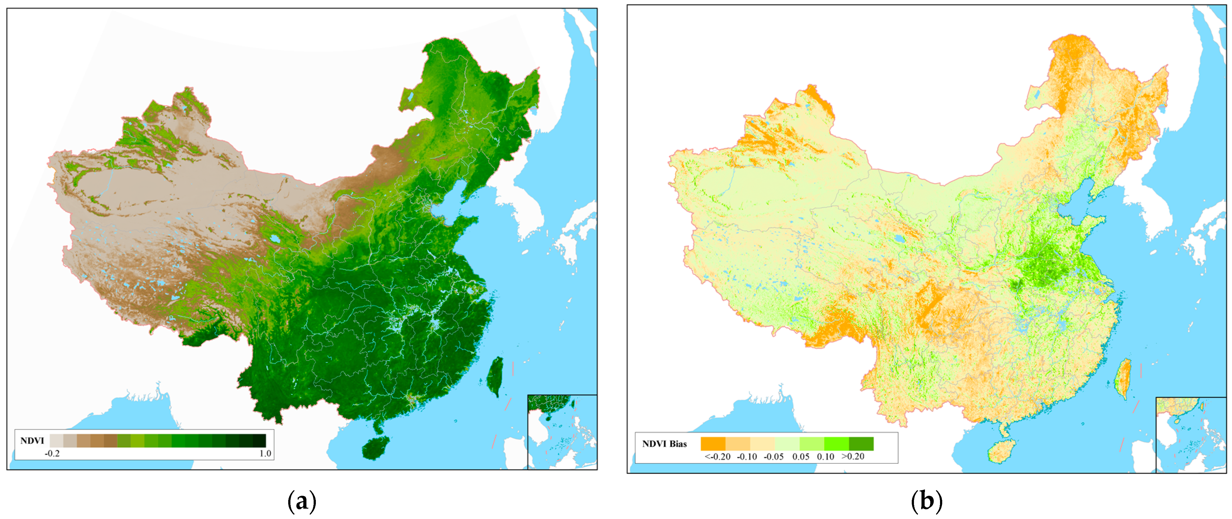
To determine the spatial distribution of the FY3D-NDVI national vegetation index, we first obtained monthly NDVI data and then combined the adult dataset using the average method. The average NDVI across China is 0.3195, as shown in Figure 3. Based on the FY-3D distribution patterns, the distribution characteristics of China’s vegetation index include a high vegetation index in the south, a low vegetation index in the northwest, a high vegetation index in the east, and a low vegetation index in the west. The average vegetation index of Northwest China ranges from 0 to 0.2, while that of North China and Northeast China is within the ranges of 0.2–0.5, and that of South China ranges from 0.6 to 0.8.
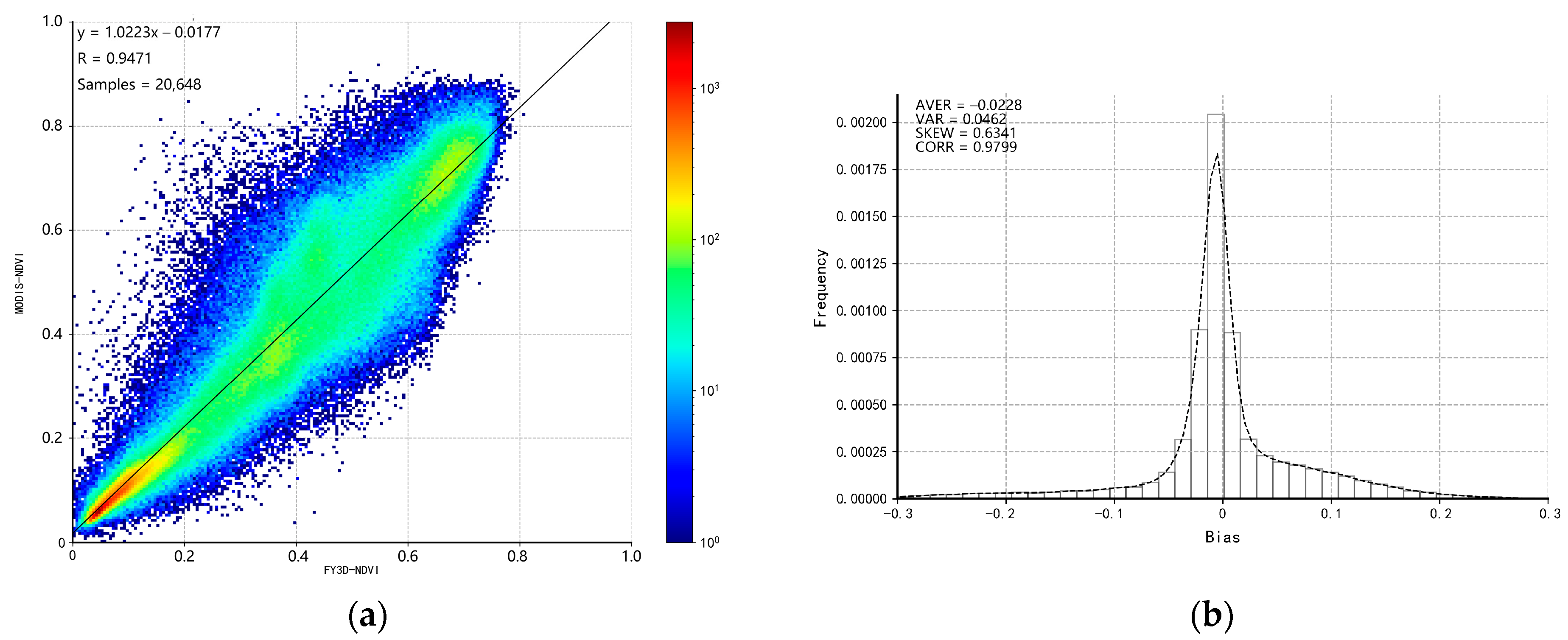
Through the comparative analysis of MODIS-NDVI in the same period, the correlation coefficient between the FNDVI and MNDVI vegetation indices was found to be 0.9471, which was in good agreement with the monitoring results of MODIS (Figure 4). The deviation analysis with MODIS monitoring showed that the FNDVI vegetation index was slightly higher (0.0615) than the MNDVI vegetation index. Among them, the vegetation index in Northeast and Southwest China was low, ranging from 0.05 to 0.1, while the vegetation index in North China and Northwest China was high, ranging from 0.05 to 0.1.

4.2. Consistency Assessment of Different Vegetation Types

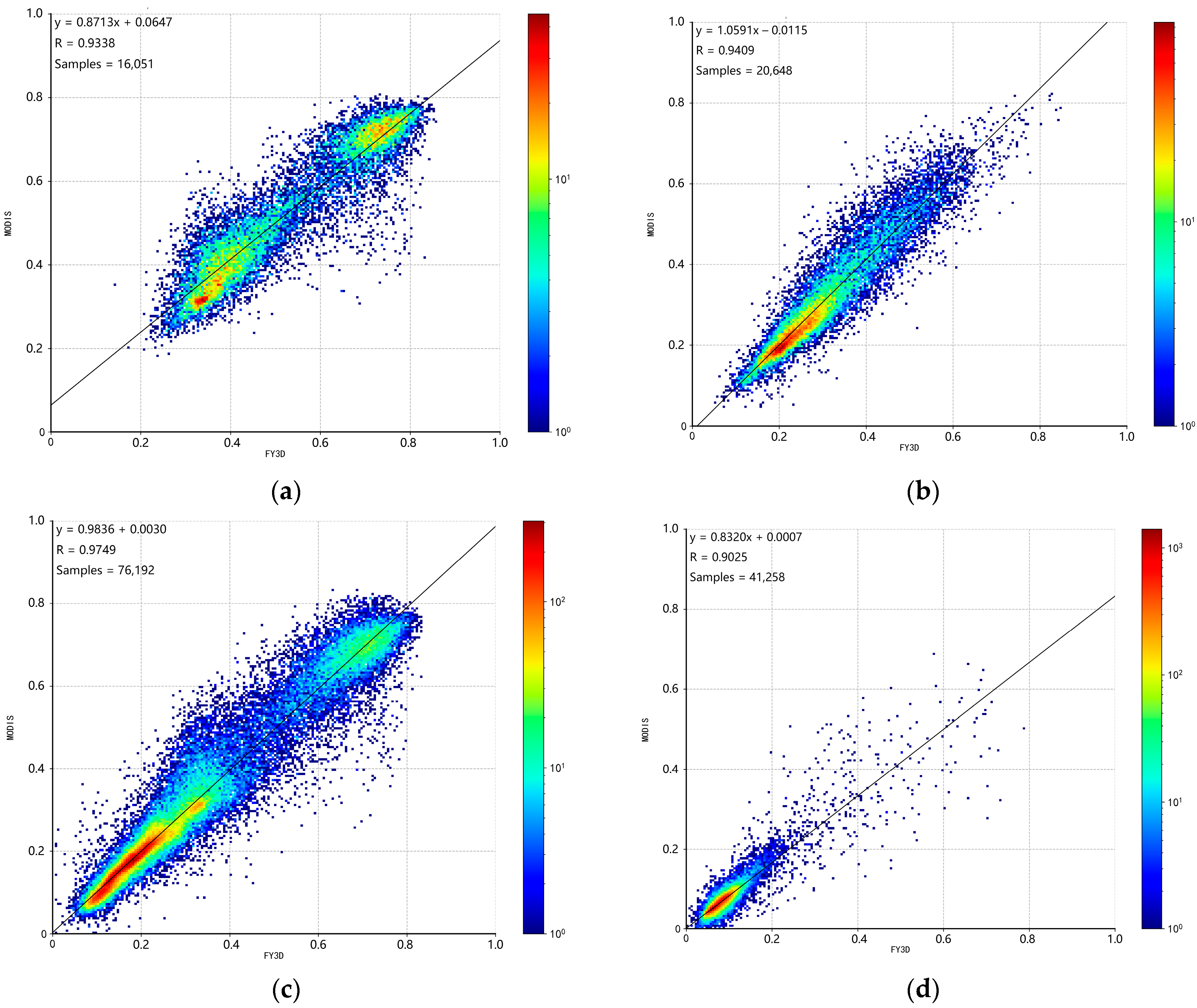
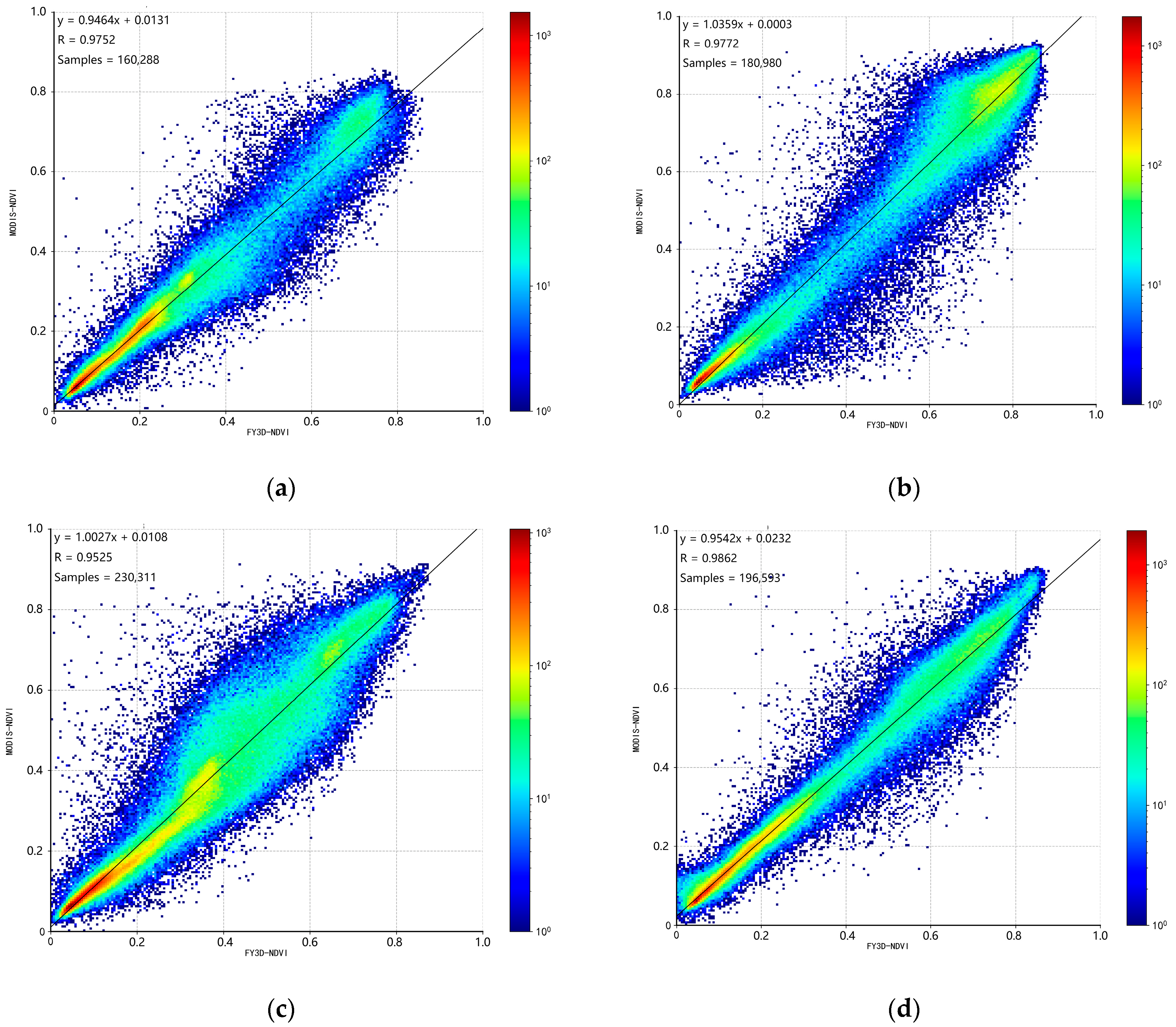
We divided the vegetation types of the surface into four categories, namely forest, farmland, grassland, and sparse grassland and desert. Through an analysis, the correlation coefficient of the forest NDVI was found to be 0.9338, while that of farmland was 0.9409. Grassland and sparse grassland and desert had values of 0.9749 and 0.9825, respectively. The national average correlation coefficient was 0.9471. The correlation of sparse grassland was found to be the best, followed by those of grassland, farmland, and forest (Figure 5).

4.3. Correlation Analysis for Different Seasons

To examine seasonal changes, we used NDVI products from January 2020, April 2020, July 2020, and October 2020 as well as January 2021, April 2021, July 2021, and October 2021, which corresponded to winter, spring, summer, and autumn. The figures below depict the statistical results of the standard deviations of MNDVI and FNDVI products. The analysis indicated that the best inversion was achieved in winter, with a correlation coefficient of 0.9862 with MNDVI, followed by summer, with a correlation coefficient of 0.9777; spring, with a correlation coefficient of 0.9752; and finally, the lowest correlation coefficient of 0.9525 for autumn (Figure 6).
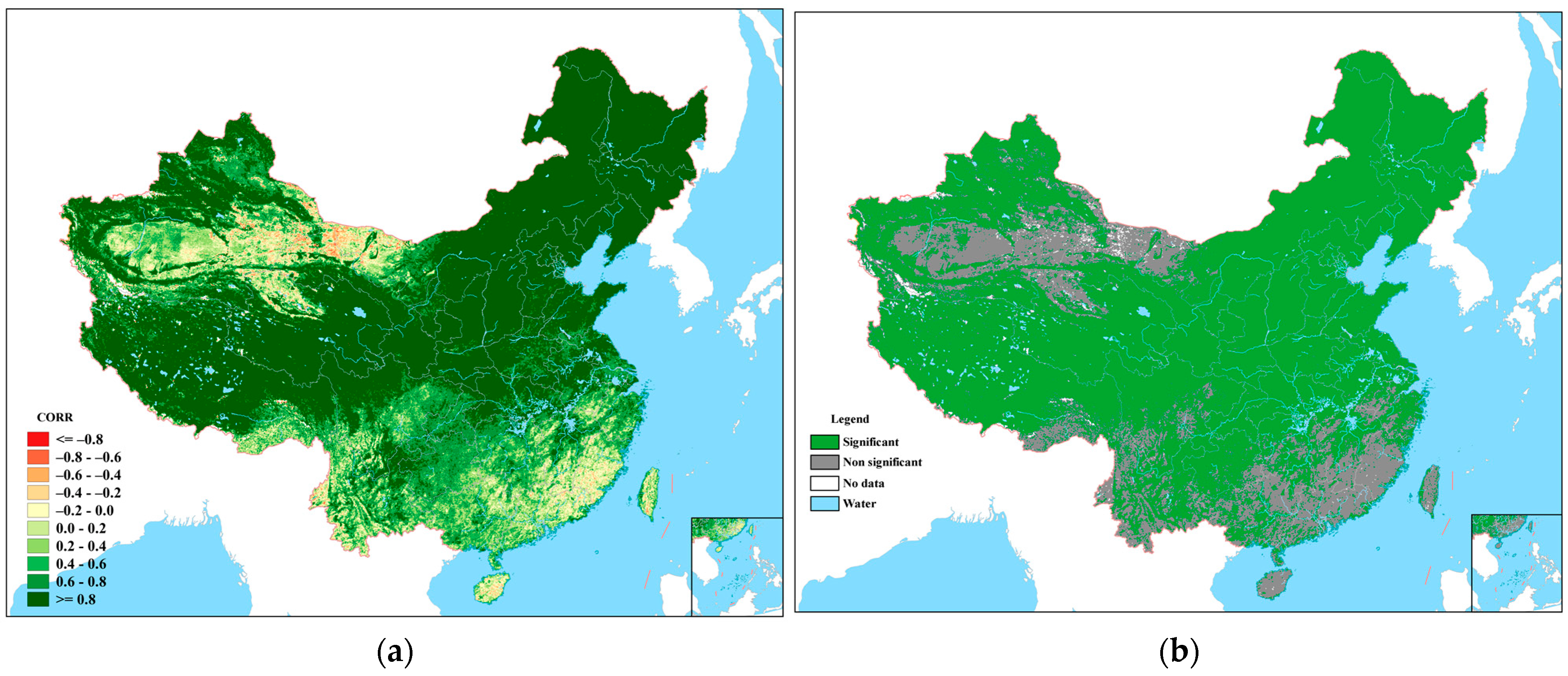
The spatial distribution consistency of FNDVI and MNDVI was tested. We evaluated the time-series consistency of these two products. The inspection period was from January 2020 to December 2021, a total of 24 months for the inspection of monthly data products. Two indicators, the correlation coefficient and the root-mean-square error, were used to evaluate the consistency of the monthly changes in the FNDVI and MNDVI data. Figure 7 shows the pixel-by-pixel spatial distribution of correlation coefficients between FNDVI and MNDVI on a monthly scale. The correlation coefficient between Northeast China, North China, and Qinghai Tibet was discovered to be high, more than 0.8. However, the correlation coefficient between Xinjiang and the desert area of Inner Mongolia was low, less than 0.4 in most cases. The correlation coefficient between the southeast coastal areas, Sichuan, Yunnan, and other regions ranged from 0.2 to 0.6. When compared to the FONDVI correlation coefficient spatial distribution map, the revised FNDVI data had a low correlation coefficient in Southern China, and the correlation coefficient in other regions was consistent with that of the FONDVI data (Figure 7a). The significance test for the FNDVI and MNDVI data was also performed pixel by pixel, and the spatial distribution results are shown in Figure 7b. Except for the non-significant correlations observed for southern Xinjiang, western Inner Mongolia, and Eastern and Central South China, the correlation was significant in most regions of the country.
As observed in Figure 7b, in the desert areas of some provinces in Xinjiang, Inner Mongolia, and Gansu, the results of the significance test revealed that the correlation was not significant. The significance test for mountainous areas of Yunnan, Tibet, Fujian, Guangdong, and other provinces showed a non-significant correlation, while other regions were significantly correlated.

4.4. Consistency Test of Typical Regional Time Series

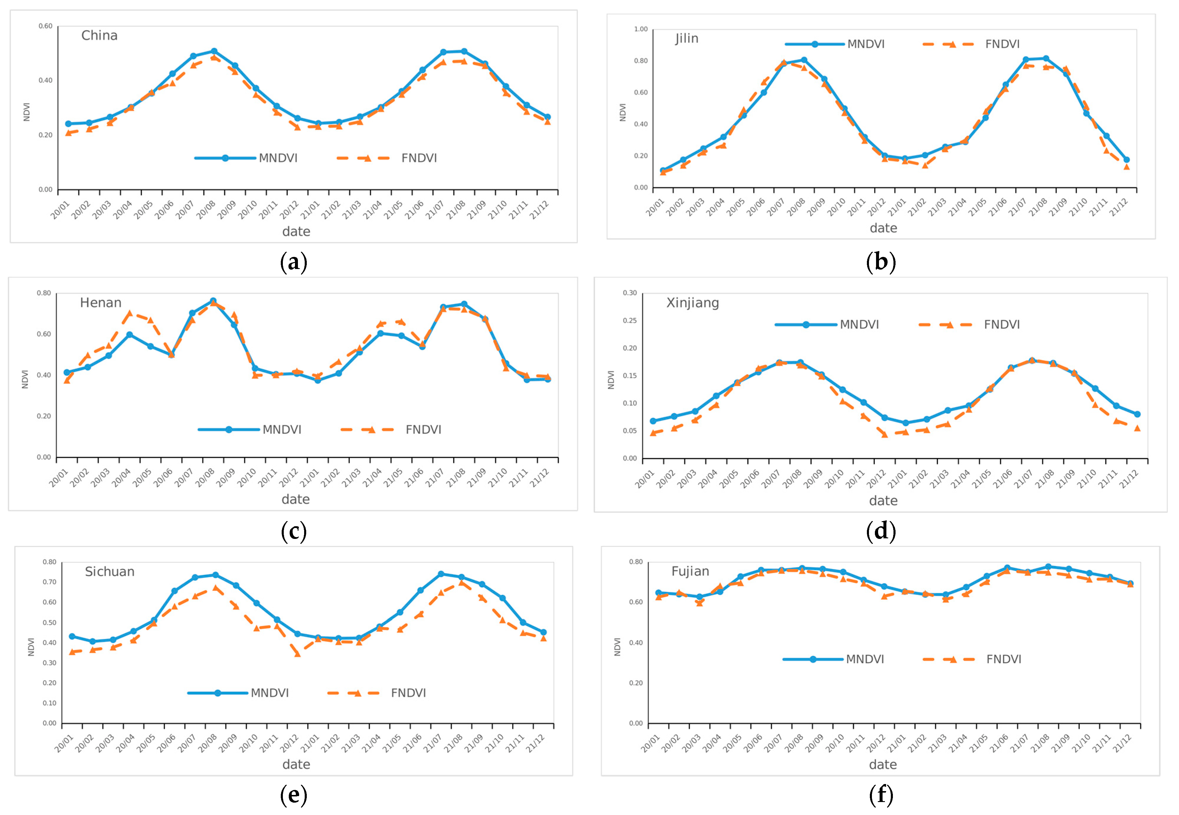
Several typical regions of China, Jilin Province, Henan Province, the Xinjiang Uygur Autonomous Region, Sichuan Province, and Fujian Province were selected, and the indices of the regional FY3D NDVI products were calculated and compared with those of the MODIS NDVI products. The results are shown in Figure 8.
Figure 8 shows that both the time-series FNDVI curve and MNDVI curve in the whole country were close to the FONDVI sequence. The FNDVI in Xinjiang was significantly improved compared with the FONDVI, which is consistent with MODIS. For Fujian Province, the FNDVI was quite different from the MNDVI, while for other provinces they were close to the MODIS curve. The main reason is that Xinjiang has limited vegetation and a low value of NDVI, while Fujian has good vegetation coverage and a high value of NDVI in a complex terrain.
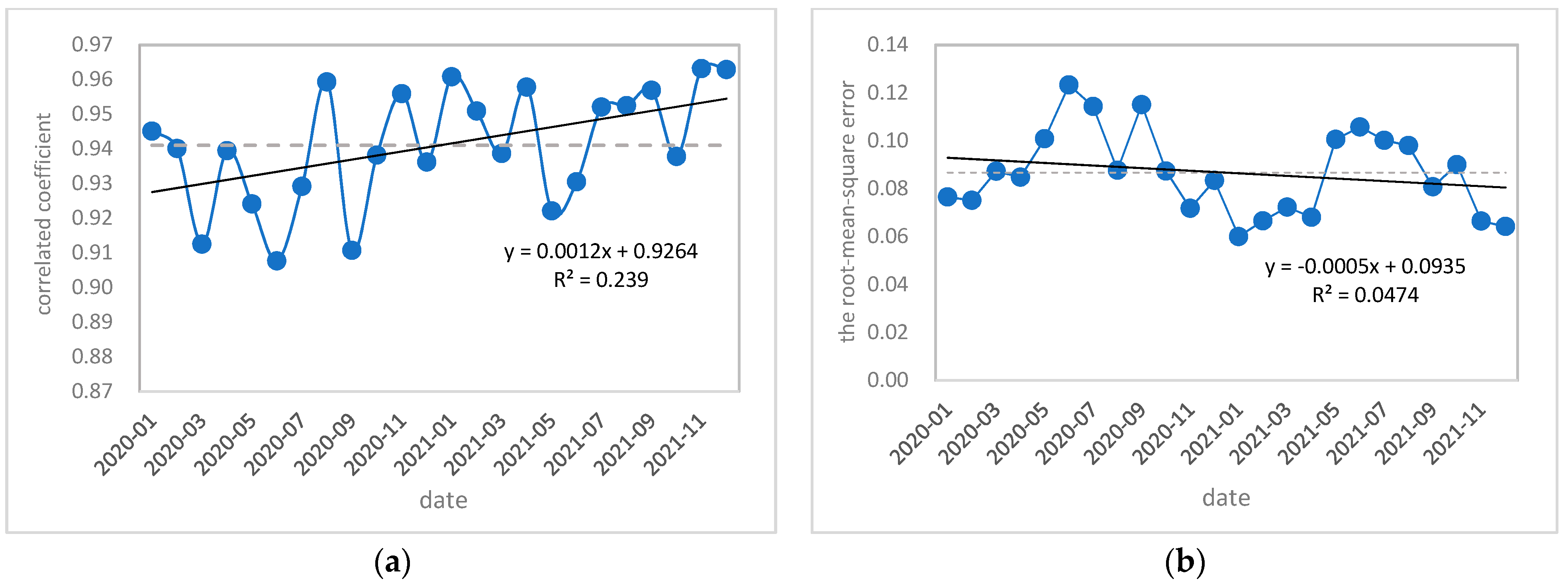
The results of the calculated standard deviation of six typical test areas are shown in Figure 9. The FNDVI data for 24 months from 2020 to 2021 were correlated on a monthly basis and plotted, as observed in Figure 9, which shows that the average value of the correlation coefficient for 24 months was 0.9410 (represented by the gray curve in the figure). The minimum value of the correlation coefficient in June 2020 was 0.9077. However, the maximum correlation coefficient value was obtained in December 2021 (0.9632). The data showed that the correlation coefficient between the FNDVI monthly products and MNDVI monthly products maintained a high value. The correlation coefficient was generally improved compared with that of the FONDVI.
As shown in Figure 9, the average value of the root-mean-square error within 24 months was 0.0867 (represented by the gray curve in the figure). The minimum value of the root-mean-square error was obtained in January 2021 (0.0600). However, the maximum root-mean-square error value was found in June 2020 (0.1233). Compared with the FONDVI root-mean-square error series, the root-mean-square error of the FNDVI decreased, indicating that the FNDVI became closer to the MNDVI products after the deviation correction.
Table 4 shows that the relative average deviation of the remaining typical areas of analysis ranged from 1.33% to 6.18%, with the largest average deviation in Sichuan and the smallest deviation in Xinjiang. The average deviation on the national scale was 2.09%. The comparison results in Table 4 show that, except for the average deviation of the FNDVI in Fujian Province, which was slightly higher than that of the FONDVI, the results of the other five regions were much better than those of the FONDVI. In particular, the average deviation of the FONDVI in Xinjiang was reduced from 36.0% to 1.3%. FONDVI’s national and regional deviations were reduced from 7.8% to 2.1%. This indicates that the deviation correction method used in this study yielded specific results and was successful in reducing the difference between the FY-3D MERSI NDVI and Aqua/MODIS NDVI products.

5. Discussion

By comparing with the MNDVI, the FNDVI values were lower than those of MODIS in the high-value region. We analyzed the spectral response function for the low/high values of MERSI/NDVI. The reflectance from dense vegetation in the red-edge area (690–740 nm) exhibited a very significant increase, and the red-light channel response function of MERSI was wider than that of MODIS, covering a small part of the red-edge area (690–700 nm), thus causing the phenomenon of the high red-light reflectance of MERSI and the low reflectance of the NDVI [23]. Jiang et al. (2011) also found that the MNDVI value tended to be high in comparison with NDVI data from the AERONET aerosol observation station [41]. The main reason is that the overestimation of aerosol concentration leads to low MODIS surface reflectance in the red bands.
The correlation coefficient of the forest NDVI was lower in these four land cover types than in agriculture, grassland, and desert, which could be attributed to topography. Forests are commonly found in high mountains, mountains, hills, and other areas with complex terrain, and topography strongly affects vegetation indices. The effects of pixel topography are mainly due to terrain shadows, reflection from adjacent terrains, sky occlusion, and alterations to the bidirectional reflectance distribution function (BRDF) of the cover type [42]. Burgess found that topography caused an error of 13.5% in NDVI data, irrespective of the angle illumination of 50 m resolution pixels [43], resulting in negative biases for their values on sun-facing slopes and positive biases on sun-backing slopes [44]. As the slope rises, topographic effects increase rapidly in strength. Topographic correction is very challenging for forests because of the geotropic growth of trees, regardless of the underlying terrain. Changes in the canopy structure also cause variations in topographic effects [45].
There is an operational system to generate FY satellite products and for their operational application. We also compared the FONDVI products and FNDVI products, which indicated that the NDVI value after the atmospheric correction was generally lower than that of the MNDVI. In comparison, the value of the FONDVI was generally higher than that of the MNDVI. By comparing the lengths in the histograms of the two products, we discovered that the median absolute deviation of the FNDVI was closer to 0, indicating that the effect after deviation correction was comparable to that of MNDVI products. Figure 10a shows that the average absolute deviation of the FNDVI was less than that of the FONDVI, indicating that after deviation correction the FY3D NDVI became more similar to the MODIS NDVI. In FONDVI products, the absolute deviation was reduced by 0.02275 from 0.067 to 0.04275, and the deviation was reduced by 36.2%. The correlation coefficients of the two products relative to MODIS products are shown in Figure 10b. The correlation coefficients of FNDVI were higher than those of FONDVI, as shown in the figure, indicating that after deviation correction the linear relationship between the FNDVI and MNDVI was stronger and their distribution was closer. The correlation coefficient increased from 0.9371 to 0.9685, with an increasing rate of 3.35%. It can be seen that the quality of the FNDVI products in this study was significantly improved based on FONDVI products.
In this study, we compared FY3D and MODIS datasets that were corrected for atmospheric effects, such as the water vapor effect. There was strong agreement between the two datasets when the atmospheric correction was applied to the data, although the MNDVI had slightly higher values. In this case, the water vapor absorption of the near-infrared (NIR) band was not the major cause of higher MNDVI values. We noticed that the reflectance of red radiation from green vegetation differed between the narrower MODIS band and the broader MERSI band. The maximum chlorophyll absorption for green vegetation was observed as a lower red reflectance in the MODIS red band. However, the MERSI (FY3D) red band (585–680 nm) covered not only the red spectra (600–680 nm) but also a portion of the green spectra (585–600 nm). Therefore, the red reflectance from green vegetation measured by the MODIS channels tended to be lower than that measured by MERSI. Therefore, the NDVI value from MODIS tended to be higher. Gitelson and Kaufman (1998) reported a detailed analysis and discussion on the difference in the red reflectance between the two sensors and its influence on NDVI values [46]. Another possible reason for the NDVI bias between FY3D and MODIS is the correction for the aerosol effect that was included in the MODIS data but not in the FY3D data [47]. Previous studies have examined the difference between FY3/MERSI and EOS/MODIS NDVI, and the results showed great linear consistency between their NDVI values [48,49].
The two datasets were generated from different satellites with different sensor designs. The differences in spectral band responses, instrument performances, and atmospheric conditions at the time of observation increased inconsistencies in measuring surface reflectance [50]. Teillet and Ren [51] pointed out that the differences in the spectral wavelengths of various sensors alone could lead to differences as large as 10% in NDVI values. Compared with MODIS, the MERSI sensor has lower radiometric and spatial resolutions and wider spectral ranges for the red and near-infrared (NIR) bands. The red bands are sensitive to chlorophyll content, influencing the NDVI value ranges [52]. The narrower NIR bands are more sensitive to atmospheric conditions; therefore, they can identify vegetation characteristics and more accurately follow the trends of vegetation changes.

6. Conclusions

We improved the F NDVI accuracy using radiative transfer, atmospheric correction, and other algorithms. Based on the MNDVI, we also calculated the correlation coefficient, mean deviation, and root-mean-square error. The spatial consistency, time consistency, and regional sequence consistency of the two products were compared. The spatial distributions of the FNDVI and MNDVI across China were very consistent at the monthly time scale. The correlation coefficients were greater than 0.9475 for the two years 2020–2021, while the average deviation was between 0.02 and 0.05, and the root-mean-square error was around 0.11. The analysis of the time consistency difference between the FNDVI and MNDVI revealed that the monthly NDVI changes of these two types of satellites were generally consistent across the country, and their change trend matched that of MODIS. Compared with the FONDVI products, the FY3D NDVI products, after the deviation correction, achieved better results in spatial distribution consistency, time consistency, and regional sequence consistency. FNDVI was closer to the MNDVI than the FONDVI in most regions of the country, and its deviation, correlation, and other indicators performed better than those of the FONDVI products. The FNDVI can be used as an operational remote-sensing product, particularly for monitoring the climate and ecology. FY-3D NDVI and MODIS NDVI products have consistent spatial distribution patterns and time-series changes. In the future, we can try to establish a long-term NDVI dataset based on these two products.

Author Contributions

Conceptualization, F.X.; methodology, Q.L. and S.L.; software, Q.L. and Y.Q.; validation, D.H. and Y.W.; data curation, S.L.; writing—original draft preparation, F.X.; writing—review and editing, F.X. and Q.L; visualization, D.H. and L.W.; supervision, Q.L.; project administration, Y.W.; funding acquisition, F.X. All authors have read and agreed to the published version of the manuscript.

Funding

This study was supported by a project of the China Three Gorges Corporation (0704182), the National Key Research and Development Plan Program (2020YFE0201900), the key innovation of CMA (CMA2022ZD03), the National Natural Science Foundation of China (NSFC Grant 52109024), and the Fengyun Satellite Climate Application Program (2022101010YE068).

Data Availability Statement

Data are available from the authors upon reasonable request as the data need further use.

Conflicts of Interest

The authors declare no conflict of interest.

References

  1. Zhou, G.S.; Wang, Y.H.; Bai, L.P.; Xu, Z.Z.; Shi, R.X.; Zhou, L.; Yuan, W.P. Study on the interaction between terrestrial ecosystems and global change. Acta Meteorol. Sin. 2004, 62, 692–707. [Google Scholar]
  2. Carlson, T.; Ripley, D. On the relation between NDVI, fractional vegetation cover, and leaf area index. Remote Sens. Environ. 1997, 62, 241–252. [Google Scholar] [CrossRef]
  3. Liu, C.; Liu, J.; Zhang, Q.; Ci, H.; Gu, X.; Gulakhmadov, A. Attribution of NDVI Dynamics over the Globe from 1982 to 2015. Remote Sens. 2022, 14, 2706. [Google Scholar] [CrossRef]
  4. Tucker, C.J. Red and photographic infrared linear combinations for monitoring vegetation. Remote Sens. Environ. 1979, 8, 127–150. [Google Scholar] [CrossRef] [Green Version]
  5. Rouse, J.; Haas, R.; Schell, J.; Deering, D. Monitoring vegetation systems in the Great Plains with ERTS. In Proceedings of the 3rd Earth Resources Technology Satellite-1 Symposium, Washington, DC, USA, 10–14 December 1973; Volume 1, pp. 309–317. [Google Scholar]
  6. Tucker, C.; Pinzon, J.; Brown, M.; Slarback, D.; Pak, E.; Mahoney, R.; Vermote, E.; Saleous, N. An extended AVHRR 8-km NDVI dataset compatible with MODIS and SPOT vegetation NDVI data. Int. J. Remote Sens. 2005, 26, 4485–4498. [Google Scholar] [CrossRef]
  7. Gamon, J.; Field, C.; Goulden, M.; Griffin, K.; Hartley, A.; Joel, G.; Penuelas, J.; Valentini, R. Relationships between NDVI, canopy structure, and photosynthesis in three Californian vegetation types. Ecol. Appl. 1995, 5, 28–41. [Google Scholar] [CrossRef] [Green Version]
  8. Jiang, H.; Xu, X.; Zhang, T.; Xia, H.; Huang, Y.; Qiao, S. The Relative Roles of Climate Variation and Human Activities in Vegetation Dynamics in Coastal China from 2000 to 2019. Remote Sens. 2022, 14, 2485. [Google Scholar] [CrossRef]
  9. Kogan, F.N. Global drought watch from space. Bull. Am. Meteorol. Soc. 1997, 78, 621–636. [Google Scholar] [CrossRef]
  10. Salinas-Zavala, C.A.; Douglas, A.V.; Diaz, H.F. Interannual variability of NDVI in northwest Mexico Associated climatic mechanisms and ecological implications. Remote Sens. Environ. 2002, 82, 417–430. [Google Scholar] [CrossRef]
  11. Piao, S.L.; Mohammat, A.; Fang, J.Y.; Cai, Q.; Feng, J.M. NDVI-based increase in growth of temperate grasslands and its responses to climate change in China. Glob. Environ. Change 2006, 16, 340–348. [Google Scholar] [CrossRef]
  12. Nathalie, P.; Jon, O.V.; Atle, M.; Jean, M.; Gaillard, C.; Tucker, J.; Nils, C.S. Using the satellite-derived NDVI to assess ecological responses to environmental change. Trends Ecol. Evol. 2005, 20, 503–510. [Google Scholar]
  13. Ren, Z. Agreement Evaluation of the NDVI Derived from AVHRR and MODIS. Geospat. Inf. 2014, 12, 125–128. [Google Scholar] [CrossRef]
  14. Xue, L.; Xian, D.; Qi, Y.G.; Xu, Z.; Qian, J.M. Test and analysis of Fenyun Satellite data service evolution indexes. Mete. Sci. Tech. 2016, 44, 692–696. [Google Scholar]
  15. Zhang, P.; Yang, H.; Qiu, H. Quantitative remote sensing from the current Fengyun 3 satellites. Adv. Meteorol. Sci. Technol. 2012, 2, 6–11. [Google Scholar]
  16. Fan, T.X. Characteristics and Functions of FY-3 Meteorological Satellite. Meteorol. Sci. Technol. 2002, 30, 321–327. [Google Scholar]
  17. Yang, J.; Dong, C.H.; Lu, N.M. FY-3A: The new generation polar-orbiting meteorological satellite of China. Acta Meteorol. Sin. 2009, 67, 501–509. [Google Scholar]
  18. Zhu, A.J.; Hu, X.Q.; Lin, M.Y. Global data acquisition methods and data distribution for FY-3D meteorological satellite. J. Mar. Meteorol. 2018, 38, 63–68. [Google Scholar]
  19. Yang, J.; Xian, D.; Tang, S.H. The latest development and application of Fengyun series meteorological satellites. Satt. Appl. 2018, 11, 8–14. [Google Scholar]
  20. Fang, J.; Tian, M.; Zhang, X.X.; Wang, Y.G. Observation of thermosphere and ionosphere using the Ionosphere PhotoMeter (IPM) on the Chinese meteorological satellite FY-3D. Adv. Space Res. 2020, 66, 2151–2167. [Google Scholar]
  21. Xu, N.; Niu, X.H.; Hu, X.Q. Prelaunch calibration and radiometric performance of the advanced MERSI on FengYun-3D. IEEE Trans. Geosci. Remote Sens. 2018, 56, 4866–4875. [Google Scholar] [CrossRef]
  22. Yang, Z.D.; Zhang, P.; Gu, S.Y. Capability of Fengyun-3D satellite in earth system observation. J. Meteorol. Res. 2019, 33, 1113–1130. [Google Scholar] [CrossRef]
  23. Wang, Y.Y.; Li, G.C. Assessment of FY-3D MERSI/NDVI global product. Acta Meteorol. Sin. 2022, 80, 124–135. [Google Scholar]
  24. Ge, M.X.; Zhao, J.; Zhong, B.; Yang, A.X. Comparison of the vegetation indexex between FY-3/VIRR, FY-3/MERSI and EOS/MODIS Data. Remote Sens. Technol. Appl. 2017, 32, 262–273. [Google Scholar]
  25. Miura, T.; Huete, A.R.; Yoshioka, H. Evaluation of sensor calibration uncertainties on vegetation indices for MODIS. IEEE Trans. Geosci. Remote Sens. 2000, 38, 1399–1409. [Google Scholar] [CrossRef]
  26. Hao, C.Y.; Ma, Y.; Zhu, Z.Z. Comparison of vegetation indices from AVHRR and MODIS in seasonal information. Geogr. Geo Inf. Sci. 2009, 25, 30–33. [Google Scholar]
  27. Jin, C. Research on land Cloud Detection Algorithm of FY-3D Satellite Spectral Imager. Ph.D. Thesis, Nanjing Information Engineering University, Nanjing, China, 2018. [Google Scholar]
  28. Wang, H.; Mao, K.; Mu, F.; Shi, J.; Yang, J.; Li, Z.; Qin, Z. A split window algorithm for retrieving land surface temperature from FY-3D Mersi-2 data. Remote Sens. 2019, 11, 2083. [Google Scholar] [CrossRef] [Green Version]
  29. Yang, Z.D.; Liu, J. A review of visible infrared imaging radiometer on meteorological satellite. J. Appl. Meteorol. Sci. 2016, 27, 592–603. [Google Scholar]
  30. Han, X.Z.; Zheng, W.; Liu, C. Estimation of chlorophyll a using MERSI and MODIS images in Taihu Lake, China. Geogr. Res. 2011, 30, 291–300. [Google Scholar]
  31. Aveni, S.; Blackett, M. The first evaluation of the FY-3D/MERSI-2 sensor’s thermal infrared capabilities for deriving land surface temperature in volcanic regions: A case study of Mount Etna. Int. J. Remote Sens. 2022, 43, 2777–2792. [Google Scholar] [CrossRef]
  32. Hu, X.Q.; Niu, X.H.; Xu, N. Improvement and application capability of fy-3d medium resolution spectral imager II. In Proceedings of the 35th Annual Meeting of the Chinese Meteorological Society, Hefei, China, 28–30 September 2018; pp. 92–100. [Google Scholar]
  33. Jiang, J.X.; Wang, M.S.; Ju, S.Y. Land surface temperature retrieval from FY-3D MERSI-2 data in the arid/semi-arid area. Adv. Geosci. 2019, 9, 693–702. [Google Scholar] [CrossRef]
  34. Vermote, E.F.; Saleous, N.Z.E.; Justice, C.O. Atmospheric correction of MODIS data in the visible to middle infrared: First results. Remote Sens. Environ. 2002, 83, 97–111. [Google Scholar] [CrossRef]
  35. Vermote, E.F.; Vermeulen, A. MODIS Algorithm Technical Background Document: Atmospheric Correction Algorithm: Spectral Reflectances (MOD09), 1999. Available online: https://lpdaac.usgs.gov/documents/305/MOD09_ATBD.pdf (accessed on 3 March 2022).
  36. Kneizys, F.X.; Shettle, E.P.; Gallery, W.O.; Chetwynd, J.H.; Abreu, L.W.; Selbry, J.E.A.; Fenn, R.W.; McClatchey, R.A. Atmospheric Transmittance/Radiance: Computer Code Lowtran 5; AFGLTR-80–0067; Air Force Geophysics Laboratory: Bredford, MA, USA, 1980. [Google Scholar]
  37. Ermote, E.F.; Saleous, N. Operational Atmospheric Correction of MODIS Visible to Middle Infrared Land Surface Data in the Case of an Infinite Lambertian Target. In Earth Science Satellite Remote Sensing; Qu, J.J., Gao, W., Kafatos, M., Murphy, R.E., Salomonson, V.V., Eds.; Springer: Berlin/Heidelberg, Germany, 2006; pp. 124–134. [Google Scholar]
  38. Jiang, Z.; Huete, A.; Wang, Y.; Lyapustin, A. Evaluation of MODIS VI Products using the AERONET-based surface reflectance validation network dataset. In Proceedings of the 34th International Symposium on Remote Sensing of Environment, Sydney, Australia, 10–15 April 2011. [Google Scholar]
  39. Xu, Y.M.; Qin, Z.H.; Chen, A.J. A pixel-by-pixel atmospheric correction algorithm for Modis Data based on Look-up Table. Geogr. Inf. Wuhan Univ. 2010, 35, 959–962. [Google Scholar]
  40. Deschamps, P.Y.; Herman, M.; Taner, D. Definitions of atmospheric radiance and transmittances in remote sensing. Remote Sens. Environ. 1983, 13, 89–92. [Google Scholar] [CrossRef]
  41. Wei, F.Y. Modern Climate Statistical Diagnosis and Prediction Technology, 3rd ed.; Meteorological Press: Beijing, China, 2009; pp. 36–56. [Google Scholar]
  42. Bai, Y.; Yang, Y.; Jiang, H. Inter comparison of AVHRR GIMMS3 g, Terra MODIS, and SPOT-VGT NDVI Products over the Mongolian Plateau. Remote Sens. 2019, 11, 2030. [Google Scholar] [CrossRef] [Green Version]
  43. Burgess, D.W.; Lewis, P.; Muller, J.P. Topographic effects in AVHRR NDVI data. Remote Sens. Environ. 2005, 54, 223–232. [Google Scholar] [CrossRef]
  44. Zhu, G.L.; Liu, Y.B.; Ju, W.M.; Chen, J.M. Evaluation of topographic effects on four commonly used vegetation indices. J. Remote Sens. 2013, 17, 210–221. [Google Scholar]
  45. Kane, V.R.; Gillespie, A.R.; McGaughey, R.; Lutz, J.A.; Ceder, K.; Franklin, J.F. Interpretation and topographic compensation of conifer canopy self-shadowing. Remote Sens. Environ. 2008, 112, 3820–3832. [Google Scholar] [CrossRef]
  46. Gitelson, A.A.; Kaufman, Y.J. MODIS NDVI optimization to fit the AVHRR data series-spectral considerations. Remote Sens. Environ. 1998, 66, 343–350. [Google Scholar] [CrossRef]
  47. Han, X.Z.; Yang, J.; Tang, S.H.; Han, Y. Vegetation products derived from Fengyun-3D Medium resolution spectral imager-II. J. Meteorol. Res. 2020, 34, 775–785. [Google Scholar] [CrossRef]
  48. Zhu, B.Q.; Huang, S.E.; Chen, X.J. Monitoring of Rice Growth based on FY3B/MERSI with AQUA/MODIS Data Contrastive Analysis. Acta Agric. Univ. Jiangxiensis 2014, 36, 1009–1015. [Google Scholar]
  49. Feng, R.; Ji, R.P.; Wu, J.W. Analysis on Difference between FY-3/MERSI-NDVI and EOS/MODIS-NDVI. Chin. Agric. Sci. Bull. 2010, 26, 359–362. [Google Scholar]
  50. Ke, Y.; Im, J.; Lee, J.; Gong, H.; Ryu, Y. Characteristics of Landsat 8 OLI-derived NDVI by comparison with multiple satellite sensors and in-situ observations. Remote Sens. Environ. 2015, 164, 298–313. [Google Scholar] [CrossRef]
  51. Teillet, P.M.; Ren, X. Spectral band difference elects on vegetation indices derived from multiple satellite sensor data. Can. J. Remote Sens. 2008, 34, 159–173. [Google Scholar]
  52. Fontana, F.; Rixen, C.; Jonas, T.; Aberegg, G.; Wunderle, S. Alpine Grassland Phenology as Seen in AVHRR, vegetation, and MODIS NDVI Time Series—A Comparison with In Situ Measurements. Sensors 2008, 8, 2833–2853. [Google Scholar] [CrossRef]
Figure 1. The main land-use types in China.
Remotesensing 15 00491 g001
Figure 2. Framework illustrating the bias correction method for the NDVI based on FY-3D MERSI-II.
Remotesensing 15 00491 g002
Figure 3. The spatial distribution of annual FY3D MERSI-II NDVI bias (a) and annual FY3D NDVI bias based on MODIS NDVI (b) during 2020 and 2021.
Remotesensing 15 00491 g003
Figure 4. Density scatter plots of FNDVI versus MNDVI (a) and the histogram of the annualized standard deviation between MODIS and FY3D MERSI-II NDVI (b) during 2020 and 2021.
Remotesensing 15 00491 g004
Figure 5. Density scatter plots of FNDVI versus MNDVI for different vegetation types: (a) forest NDVI, (b) agriculture NDVI, (c) grassland NDVI, (d) desert NDVI.
Remotesensing 15 00491 g005
Figure 6. Density scatter plots of FNDVI versus MNDVI in different seasons, including (a) spring, (b) summer, (c) autumn, and (d) winter.
Remotesensing 15 00491 g006
Figure 7. Spatial distribution of the correlation coefficient between FNDVI and MNDVI (a) and the statistical significance test for the spatial distribution (b).
Remotesensing 15 00491 g007
Figure 8. Comparison of the regional average real sequence of monthly FNDVI and MNDVI values in China from 2020 to 2021.
Remotesensing 15 00491 g008
Figure 9. Comparison of the (a) coefficient of variation and (b) root-mean-square error between FNDVI and MNDVI from January 2020 to December 2021.
Remotesensing 15 00491 g009
Figure 10. Comparison of the average absolute deviation (a) and correlation coefficient (b) between FONDVI and FNDVI products relative to MNDVI.
Remotesensing 15 00491 g010
Table 1. The characteristics of MERSI-II bands.
BandCentral Wavelength (µm)Spatial Resolution (m)SNR NE∆T
(K)
Application of this Algorithm
10.47250100Aerosol retrieval algorithm
20.55250100
30.65250100Aerosol retrieval algorithm and NDVI calculation
40.865250100Aerosol retrieval algorithm and NDVI calculation
51.381000100
61.641000200
72.131000100Aerosol retrieval algorithm
80.4121000300
100.491000300
110.5551000500
120.671000500
130.7091000500
140.7461000500
150.8651000500
160.9051000200
170.9361000100
180.941000200
191.031000100
203.810000.25 K
214.0510000.25 K
227.210000.30 K
238.5510000.25 K
2410.82500.4 K
25122500.4 K
Table 2. Water vapor absorption coefficients in the first four bands of the MERSI sensor of the meteorological satellite FY-3D.
Band NameCentral Wavelength (nm) A H B H
4700.00000.0000
B25500.00000.0000
B3650−5.60720.8202
B4865−5.252510.7252
Table 3. The optical thickness of atmospheric molecules based on FY-3D MERSI-II data.
Band NameCentral
Wavelength (nm)
Atmospheric Molecular Optical Thickness, τ
EV_250_RefSB_b14700.188128
EV_250_RefSB_b25500.0984957
EV_250_RefSB_b36500.0529696
EV_250_RefSB_b48650.0156664
Table 4. FNDVI deviations compared with the MNDVI in different regions of China.
Data (yy/mm)JilinFujianHenanSichuanXinjiangChina
20/010.01120.02120.03850.07650.02130.033
20/020.03630.01010.05930.04120.02140.0226
20/030.02350.03140.04990.0370.01580.021
20/040.05340.03020.10590.04460.0160.0015
20/050.03850.13170.12830.01430.00010.0047
20/060.06630.11480.00320.07620.0070.0342
20/070.01020.10140.03290.09290.00020.0335
20/080.04950.11190.01050.06260.00490.0223
20/090.03040.12310.05140.10390.00260.0224
20/100.02720.03420.03380.12260.02060.023
20/110.02230.01680.00280.02970.0240.0227
20/120.01940.04880.01310.09820.03020.0326
21/010.01640.00210.02110.00610.01620.0115
21/020.06380.0060.05780.01730.0190.0143
21/030.01430.02350.02220.02110.02440.0184
21/040.01030.03340.04810.0080.00670.0048
21/050.04080.1280.06950.08360.00220.0114
21/060.02570.15510.01550.11750.0010.0245
21/070.03940.0920.0080.09220.00130.0361
21/080.05410.13830.02570.0270.00070.0361
21/090.03510.05120.00630.06620.00210.0071
21/100.04670.06050.02240.10730.02920.0239
21/110.0920.01020.02230.05030.02710.0232
21/120.04340.00690.01380.0290.02490.0167
Absolute deviation0.03630.06180.03590.05940.01330.0209
Relative deviation3.63%6.18%3.59%5.94%1.33%2.09%
Disclaimer/Publisher’s Note: The statements, opinions and data contained in all publications are solely those of the individual author(s) and contributor(s) and not of MDPI and/or the editor(s). MDPI and/or the editor(s) disclaim responsibility for any injury to people or property resulting from any ideas, methods, instructions or products referred to in the content.