FERA-Net: A Building Change Detection Method for High-Resolution Remote Sensing Imagery Based on Residual Attention and High-Frequency Features

Abstract

Buildings can represent the process of urban development, and building change detection can support land use management and urban planning. However, existing building change detection models are unable to extract multi-scale building features effectively or fully utilize the local and global information of the feature maps, such as building edges. These defections affect the detection accuracy and may restrict further applications of the models. In this paper, we propose the feature-enhanced residual attention network (FERA-Net) to improve the performance of the ultrahigh-resolution remote sensing image change detection task. The FERA-Net is an end-to-end network with a U-shaped encoder–decoder structure. The Siamese network is used as the encoder with an attention-guided high-frequency feature extraction module (AGFM) extracting building features and enriching detail information, and the decoder applies a feature-enhanced skip connection module (FESCM) to aggregate the enhanced multi-level differential feature maps and gradually recover the change feature maps in this structure. The FERA-Net can generate predicted building change maps by the joint supervision of building change information and building edge information. The performance of the proposed model is tested on the WHU-CD dataset and the LEVIR-CD dataset. The experimental results show that our model outperforms the state-of-the-art models, with 93.51% precision and a 92.48% F1 score on the WHU-CD dataset, and 91.57% precision and an 89.58% F1 score on the LEVIR-CD dataset.

1. Introduction

Buildings are a significant component of urban development, and building change detection is commonly utilized in land use management [1], illegal building management [2], and urban development [3]. Change detection (CD) aims to analyze multitemporal images within the same region and detect the process of object or phenomenon differences within the region [4]. Remote sensing images can be used for identifying and evaluating surface changes utilizing obtained multitemporal images covering the same surface region and its accompanying data [5]; this is one of the most active areas of research in the remote sensing field. With the development of remote sensing technology, a substantial chunk of remote sensing data are now accessible, providing substantial information about land cover [2]. The development of computing and AI technology also provides a great deal of theoretical guidance for CD methods. The CD methods can be divided into two categories: pixel-based and object-based methods [6].

Due to their resolution limitations [7], pixel-based methods for change detection in remote sensing images became mainstream. These methods compare pixels between multiple temporal images [8,9] to produce change maps using clustering techniques [10,11] or threshold segmentation [12,13]. The main classifiers used include support vector machines [14], random forests [15], and k-nearest neighbor classification [16], etc. However, they ignore contextual information and are prone to noise [17]. Object-based methods were introduced to take advantage of the spatial contextual relationships in these images. As a result, these techniques are frequently utilized for jobs involving the CD of low- and medium-resolution remote sensing images [18]. These methods use local clusters of labeled pixels called “objects” to reduce false positives and missing values in change maps [19]. They effectively remove noise and misaligned images by segmenting images into homogeneous regions using spectral and spatial adjacency similarities and then generating change result maps based on the texture, shape, and spatial relationships of neighboring objects [20,21,22,23]. However, the precision of object-based CD models is impacted by the segmentation procedure, and they often require manual intervention and are not robust.

Due to breakthroughs in the computer vision field, deep learning networks have been applied to remote sensing image analysis [24,25]. Deep learning networks are applied to the CD task to automatically extract the relevant semantic features and obtain an abstract feature representation of the image information. Compared with traditional methods, deep-learning-based approaches can automatically learn features, which significantly reduces the need for specialized domain knowledge. The performance of CD tasks has greatly improved profits owing to the excellent performance of deep learning models in capturing and representing image features. This has resulted in a new era of CD technologies. The CD network framework consists of three main parts: feature extraction, network optimization, and accuracy evaluation. From the perspective of feature extraction, the CD methods can be classified into five major types: autoencoder (AE)-based, recurrent neural network (RNN)-based, generative adversarial network (GAN)-based, convolution neural network (CNN)-based, and transformers-based methods [7]. AE is an artificial neural network used in semi-supervised and unsupervised learning to learn representations of input information by using it as a learning target. Liu et al. [26] propose a stacked autoencoder for synthetic aperture radar change detection that effectively adapts to the multiplicative noise environment present in SAR change detection. RNN generates CD results by learning multitemporal image features and establishing change relationships between multi-period sequence remote sensing images [27,28]. Lyu et al. [29] build on RNN using an improved LSTM approach to design a change rule with transferability to provide reliable change information for multitemporal images. GANs can be trained with a small amount of real data and generate a large amount of pseudo-data through adversarial learning, thus enhancing the network’s generalization ability [30,31]. Peng et al. [18] used multitemporal images as input to UNet++ to generate multi-level feature maps of predicted change maps. Multiple side-output fusion (MSOF) was then introduced to generate the final variogram. Fang et al. [32] proposed SUNNet-CD, a tightly connected Siamese network for CD tasks, with deep supervision of the network training by aggregating and refining semantic information at different levels. Transformer-based methods are an effective attention-based approach to improve CD results by capturing global contextual information and establishing remote target dependencies [33]. Wang et al. [25] proposed TransCD by adding the transformer structure to the feature difference network to improve the robustness to noisy changes by establishing global semantic information. The CD methods are roughly divided into two categories, the early fusion (EF) strategy and the late fusion (LF) strategy, from the perspective of the feature fusion strategy [34]. The authors of [35] design a CD network with EF strategies based on UNet networks, use skip connections to improve accuracy, and explore the impact of different fusion strategies on network performance by varying the feature fusion. In [36], the Siamese network is used to extract the dual-time image features, and the boundary integrity of the resultant map is improved based on an LF strategy using multi-level depth features fused with differential features through an attention mechanism. Studies have shown that late fusion strategies give better CD results than early fusion strategies.

There has been a growing interest in researching multi-scale features for building change detection in remote sensing images in recent years. This is due in part to the increasing resolution of remote sensing images, which allows for more detailed and accurate detection of changes in buildings. Previous methods, such as pixel-based and object-based approaches, have been effective in detecting changes in low- to medium-resolution images, but may not fully utilize the multi-scale information available in high-resolution images [37]. Thus, there is a need to develop methods that can effectively extract multi-scale building features from high-resolution images in order to improve the accuracy of building change detection. Research in this area has included the use of deep learning methods, such as convolutional neural networks, to extract and utilize multi-scale features in building change detection [34]. However, there are still challenges to be addressed, such as the information gap between upper and lower layers of the network and the difficulty in fully utilizing the local and global information of the feature maps [38]. Further research in this area is necessary in order to improve the performance and efficiency of building change detection in high-resolution remote sensing images.

Although deep learning methods have achieved great advantages in CD tasks, there are still some problems to overcome. On the one hand, while current building change detection methods consider multi-scale features, they are often unable to fully utilize both global and local information in multi-scale feature maps. Due to successive downsampling operations in the encoder part and successive upsampling operations in the decoder part, detailed information such as building boundary information and multi-scale buildings is gradually diluted. On the other hand, the existing CD networks tend to connect only sibling feature maps when passing contextual information through skip connections. This leads to an information gap between the upper and lower layers when the network is connected, which cannot fully utilize the local and global information of the feature maps, thus affecting the efficiency of feature extraction and limiting the performance of the model.

The following is a summary of this paper’s significant contributions.

(1)

In order to fully utilize the high-frequency information in remote sensing images to enhance building edges and extract multi-scale features through multi-level feature maps, we propose a new CD network called FERA-Net, using a Siamese network to detect building changes at the pixel level. The network can extract multi-level and multi-scale features from dual-time remote sensing images.

(2)

We designed a hierarchical attention-guided high-frequency feature extraction module (AGFM) to effectively capture building information in remote sensing images. The AGFM uses the residual attention mechanism and the high-frequency information enhancement module to effectively capture building features while enhancing building boundary information and mitigating the effect of noise. We used the feature-enhanced skip connection module (FESCM) to fuse the local and global information of the dual-temporal image differential maps, aggregating differential map features of different levels and scales to capture building information at different scales in terms of fusion strategy selection. To better perform change monitoring, we designed a hybrid loss function to focus on building change information and a priori boundary information.

(3)

We conducted experiments on two publicly available datasets to evaluate the performance of FERA-Net in remote sensing CD tasks in multiple aspects. Both quantitative and qualitative comparison results show the significant advantages of FERA-Net compared with other network models.

The remainder of this paper is structured as follows. The work related to CD is described in Section 2. The details of the FERA-Net are described in Section 3. The dataset and experimental setup are presented in Section 4. Comparative and ablation experiments are described and discussed in Section 5. Section 6 summarizes the work conducted in this paper and future perspectives.

2. Related Work

2.1. Change Detection Networks with Siamese Network

Siamese networks are connected architectures of two structurally identical neural networks that share weights. These networks accept two separate inputs and produce representations of the high-dimensional spaces they are embedded in. Change detection tasks aim to discover the difference between changed and unaltered pixels in multitemporal images. The features from multitemporal images are extracted using the two branches of the Siamese network. Then, the network creates the change maps based on the similarity between the two attributes. This makes the Siamese network a strong contender for applications of change detection. Caye Daudt et al. [35] designed a CD network based on a single-branch structure and a CD network based on a Siamese structure and experimentally demonstrated the performance improvement of the Siamese network for the CD task. Chen and Shi et al. [39] exploit the spatial–temporal relationships that exist between remote sensing image pixels, design a self-attentive module to model the spatial–temporal relationships, and extract diachronic image spatial–temporal features based on Siamese networks.

2.2. Change Detection Networks with Skip Connection

The encoder–decoder architecture is a common network architecture for change detection. However, when the encoder part extracts the image features through downsampling operations such as convolution, the detailed information of the remote sensing image is easily lost. Therefore, connecting the encoder and decoder with direct information through skip connection can help the decoder to better recover space information and improve the change detection performance. As a result, UNet and its variants, which were the first to use skip connections, are widely used in CD tasks. Ji et al. [40] designed a UNet structure for pixel segmentation incorporating multi-scale aggregation to help recover spatial information. Based on UNet++, Fang et al. [32] combined NestedUNet and Siamese networks to propose SNUNet-CD, which maintains high-resolution features and fine-grained localization information through a skip connection mechanism. D. Peng et al. [41] added an attention mechanism to the UNet++ dense skip connection to reduce the semantic gap between high-level features and the underlying features and to facilitate the extraction and fusion of multi-scale features. The experiment verified that dense skip connections are used in the decoding phase to efficiently fuse different features. Although using skip connections and dense skip connections in UNet and UNet++ can help to recover spatial information, these networks only transfer information between sibling feature maps and do not make full use of full-size feature map information.

2.3. Change Detection Networks with Attention Mechanism

The fundamental concept behind the attention mechanism is to emphasize certain crucial aspects while suppressing unimportant ones based on the association between the original data [42]. By using cross-channel correlations and spatial interactions between features, creating channel attention maps and spatial attention maps, networks can concentrate on where the information is located. This process enables the rapid filtering of high-value information from the mass of information using limited attentional resources. Attentional mechanisms are widely used with change detection networks. Chen et al. [43] designed DASNet to improve the model’s performance by capturing long-range dependencies through a dual-attention mechanism to obtain more feature representations. Ma et al. [44] designed a multi-attentive cued feature fusion network for change detection tasks, introducing coordinate attention (CA) via a Feature Enhancement Module (FEM) to obtain more accurate position and channel relationships. J. Chen et al. [45] proposed MSF-Net, which uses an attention mechanism to fuse contextual information to obtain rich global contextual information about a building and effectively suppress irrelevant features.

3. Methods

3.1. Overview

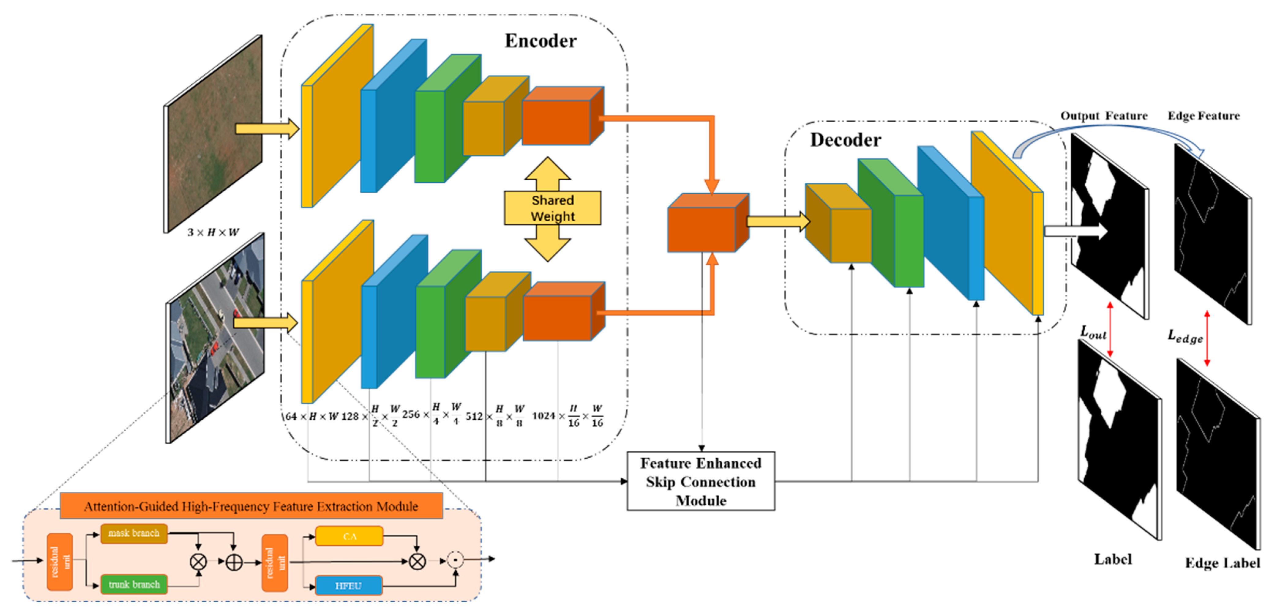
As shown in Figure 1, we designed the network with a typical encoder–decoder architecture called FERA-Net. The AGFM is stacked together in the encoder part to extract features from bitemporal images. In this module, we use the residual spatial attention mechanism for concentrating building change areas and the residual channel attention mechanism to improve the edge features and high-frequency information extracting. The FESCM is utilized to aggregate the change features from the multi-scale feature maps, and then the module transmits the features to the decoding part. It provides spatially detailed information from the low-level feature maps and the semantic information from the high-level feature maps to make up for the information loss caused by downsampling in the encoder part, so that the network can completely mine the multi-scale characteristics at multiple levels. The final-layer feature map of the decoder part is used to generate the final change result map and is also used to extract building edge estimates and construct the hybrid loss function to accomplish accurate segmentation for the edges of the change map.

3.2. Encoder Part

Buildings in bitemporal images often possess different features, the changing characteristics of which cannot be fully described by only using one level of feature maps. Thus, we use a multi-layer approach to mine different types of feature information. Considering that we are using a pair of dual-time images as input data, we introduce the Siamese network to implement the feature extraction task in the coding part. Specifically, the Siamese network uses two different inputs to extract deep-level features through two similar subnetworks with the same architecture, parameters, and weights, and can also be used to describe the dual-time image features. As shown in Figure 1, when a pair of dual-time images of size $3\times H\times W$ is used as input, the network we designed obtains the corresponding five-layer feature maps through five AGFMs, denoted as $F_1$, $F_2$, $F_3$, $F_4$, and $F_5$, which have dimensions of $64\times H\times W$, $128\times \frac{H}{2}\times \frac{W}{2}$, $256\times \frac{H}{4}\times \frac{W}{4}$, $512\times \frac{H}{8}\times \frac{W}{8}$, and $1024\times \frac{H}{16}\times \frac{W}{16}$, respectively, which are used to generate coarse-grained feature maps with high resolution and fine-grained features with low resolution.

3.2.1. Attention-Guided High-Frequency Feature Extraction Module

Buildings are manufactured objects with obvious edges. In the end-to-end network, the building boundary information is always weakened, and it is difficult to recover the building boundary due to its network characteristics, which often lead to the blurring of the edges of buildings during building change detection [46].

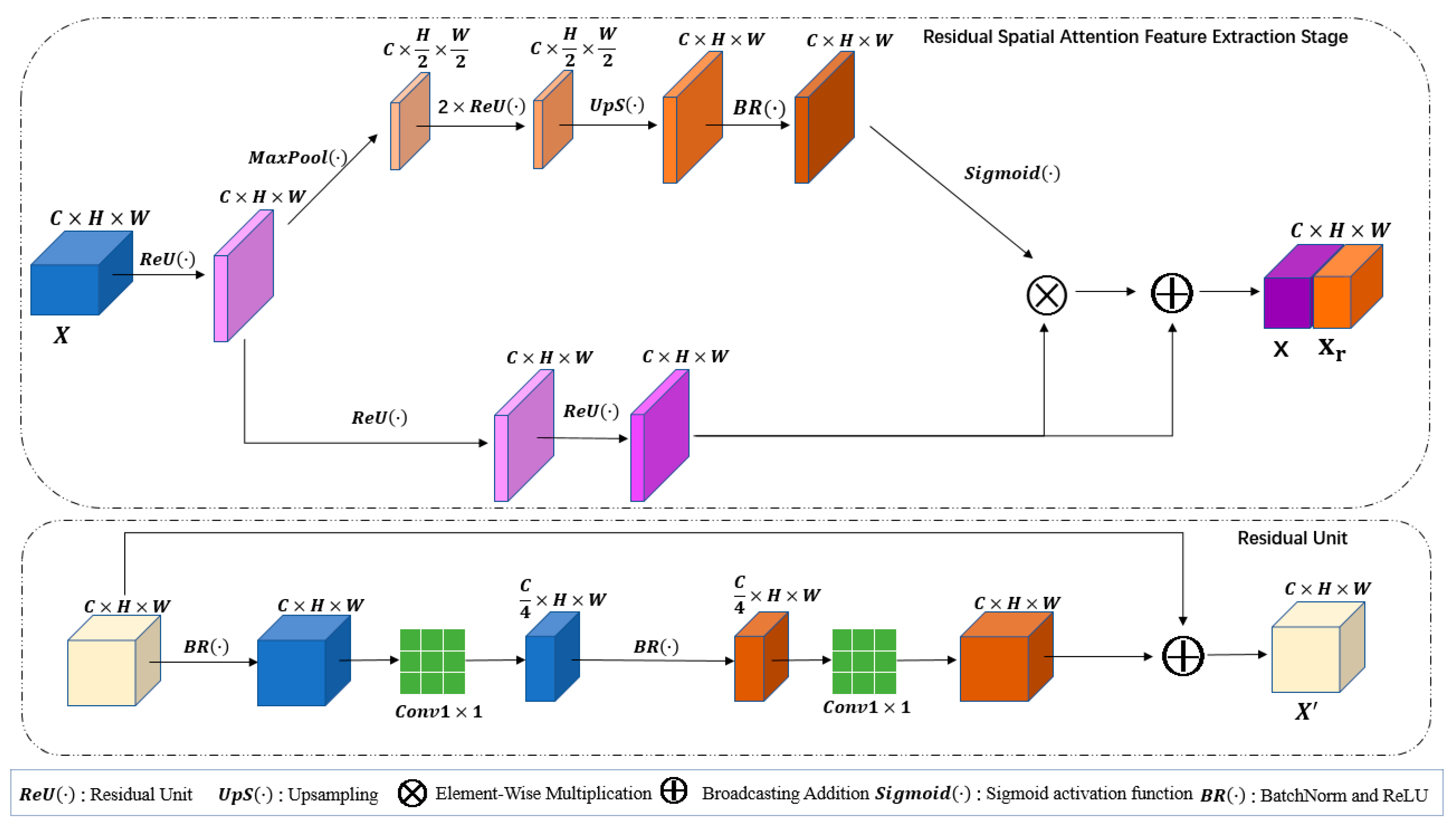
However, the identification of building edges is essential in building change detection and greatly impacts the final detection accuracy. In remote sensing images, the high-frequency signal corresponds to the part of the image that changes drastically, which indicates the edges (contours) or noise in the image. Therefore, if the high-frequency features of remote sensing images are enhanced, we can recover the edge information of buildings to some extent, but this will also enhance the other high-frequency features, such as noise. To address this issue, we integrate the attention method into the building change detection network. The AGFM is designed to identify areas of building change and retain building boundary information. The detailed AGFM structure diagram is shown in Figure 2.

3.2.2. Residual Spatial Attention Feature Extraction Stage

Not every region in the image contributes equally to the building change detection task; we focus only on the regions of building change in our study [47]. Therefore, it is necessary to apply spatial attention mechanisms to the task of change detection. The spatial attention mechanism reduces the effect of noise by generating a spatial attention map that focuses on the changing building regions in the remotely sensed image. In the RSAS module, we divide the attention module into the mask branch and the trunk branch. The trunk branch is used for feature extraction, and the mask branch uses a top-down structure to learn to generate spatial attention masks. The trunk branch output $F\left(x\right)$ with input $x$ is given to the mask branch. The output of the attention mask is

$$H_{i,c}\left(x\right)=M_{i,c}\left(x\right)\times F_{i,c}\left(x\right)$$

(1)

where $i$ ranges over all spatial positions and $c\in \{1,\dots ,C\}$ is the index of the channel.

The attention calculated by the above equation is differentiable, and the attention that can be differentiated can be learned by the neural network by calculating the gradient and by forward propagation and backward feedback to obtain the weight of the attention. Thus, the attention mask can be used as a filter for gradient updates during backpropagation. In the mask branch, its gradient is:

$$\frac{\partial M(x,\theta )F(x,\varnothing )}{\partial \varnothing }=M(x,\theta )\frac{\partial F(x,\varnothing )}{\partial \varnothing }$$

(2)

where $\theta$ represents the mask branch parameters and $\varnothing$ represents the trunk branch parameters. By generating spatial attention $M\left(x\right)$ through the mask branch structure, the effect of noise in the image on the identification of changing regions can be effectively reduced.

However, merely stacking attention modules will lead to performance degradation, so we use residual learning in the spatial attention module. As shown in Figure 3, the output of the modified attention module is

$$H_{i,c}\left(x\right)=(1+M_{i,c}\left(x\right))\times F_{i,c}\left(x\right)$$

(3)

where $M\left(x\right)$ ranges from $\left[\mathrm{0,1}\right]$, with $M\left(x\right)$ approximating 0 and $H\left(x\right)$ approximating the original features, $F\left(x\right)$. $M\left(x\right)$ work as a feature selector, which enhances good features and suppresses noise from trunk features. This process is referred to as attention residual learning.

3.2.3. Residual Channel Attention High-Frequency Feature Enhancement Stage

In building CD tasks, the edges of buildings are often areas of dramatic change, often consisting of high-frequency features in the image, and identifying these is important. Due to the variety of building shapes in remote sensing images, the isotropic Sobel operator is more suitable for extracting high-frequency features [46]. As shown in Figure 4, after acquiring the high-frequency features representing the edges of buildings, we use the channel attention to add the extracted high-frequency information to the network. The channel attention typically consists of a direct, global average pooling of information within a channel, and it ignores local information within each channel. The feature compression along the spatial dimension turns each two-dimensional feature channel into a real number with a global perceptual field, in which the output dimension matches the number of input feature channels using global average pooling. Formally, for the output of the modified attention module $X\in {\mathbb{R}}^{C\times H\times W}$, the global average pooling $G\left(X\right)$ can be obtained as follows:

$$G(X)=\frac{1}{H\times W}\sum _{i=1}^H\sum _{j=1}^{W}X(i,j)$$

(4)

We chose the simple gate control mechanism with a sigmoid activation function to aggregate information for capturing the correlation between channels, as shown in the following formula:

$$F_{CA}\left(X\right)=\xi \left(FC\left(\delta \left(FC\left(G\left(X\right)\right)\right)\right)\right)$$

(5)

where $\delta$ denotes the ReLU function, $\mathrm{\xi }$ denotes a sigmoid activation function, and $\mathrm{F}\mathrm{C}\left(\bullet \right)$ denotes fully connected layers.

In addition, we use the isotropic Sobel operator to extract high-frequency features, as shown in the following formula:

$$F_{HF}(X)=Mean\left(\sum _{i=1}^8{S}_i\left(X\right)\right)$$

(6)

Finally, the extracted high-frequency features need to be fused with the channel information in the channel attention, as shown in the following formula:

$$F_{RC}\left(X\right)=X\oplus F_{CA}\left(X\right)$$

(7)

$$F_{RCA}\left(X\right)={Conv}_{1\times 1}\left(Cat\left(H\left(X\right)\oplus ResC\left(X\right)\right)\right)$$

(8)

where $Cat\left(\bullet \right)$ denotes channel-wise concatenate, ${Conv}_{1\times 1}$ denotes a 1 × 1 convolution operation, and $\oplus$ denotes element-wise addition.

3.3. Decoder Part

In the coding section, we extracted five levels of diachronic remote sensing image feature maps. In the decoding part, we enhanced the predictive power of the model by aggregating full-scale features through the FESCM to mine the building change features between the dual-temporal image feature maps.

3.3.1. Feature-Enhanced Skip Connection Module

Skip connections are frequently employed in change detection tasks to link low-level feature maps and high-level feature maps for improving a network’s capacity for prediction. However, the UNet-based model connects only sibling feature maps, which makes it difficult to examine enough data from the full scale and renders the placement and borders of buildings unclear. In order to reduce the differential information of buildings, aggregate local and global feature contexts, and learn feature representations from the multi-scale aggregated feature maps, we propose the FESCM to aggregate the full-scale feature maps produced by $F_{t1}$ and $F_{t2}$. Furthermore, since different depths of perceptual fields are not equally sensitive to targets of different sizes (shallow layers are more sensitive to small targets, and deep layers are more sensitive to large targets), we stitch them together by feature concatenation to integrate the advantages of both. In addition, as the number of network layers increases, one layer of downsampling will keep losing information (large object edge information and small objects themselves), so the features with small receptive fields are supplemented to make the location information more accurate.

As shown in Figure 5, we take the third layer feature map $X_{De}^3$ in the network as an example, and the steps are as follows:

• The low-level feature maps $F_{t1}^1,F_{t2}^1,F_{t1}^2,\mathrm{a}\mathrm{n}\mathrm{d}{F}_{t2}^2$ preserve the detailed information, fusing the fine-grained semantics. $F_{t1}^1,F_{t2}^1,F_{t1}^2,\mathrm{a}\mathrm{n}\mathrm{d}{F}_{t2}^2$ are to be downsampled to the same scale as $F_{t1}^3$ to unify the size. This is followed by a 3 × 3 convolution with 64 channels. The downsampling in this part is performed using overlap-free maximum pooling.
• The feature map of the same scale encoder, the $F^3$ layer, is directly operated by a 3 × 3 convolution with 64 channels.
• The high-level feature maps $X_{De}^4$ and $X_{De}^5$ are upsampled by 2× and 4×, respectively, to ensure the uniformity of the feature map size. The upsampling of this part is achieved by bilinear interpolation.

Five layers are stacked (stitched and fused) to form a 320-channel feature map. The feature map generation process of other decoding parts is similar, which is calculated as follows:

$$X_{De}^i=\left\{\begin{array}{c}FEM\left(F_{t1}^i,F_{t2}^i\right), i=N\\ {\displaystyle \sum _{k=1}^{i-1}}Down\left(FEM\left(F_{t1}^k,F_{t2}^k\right)\right)+BR\left(FDEM\left(F_{t1}^i,F_{t2}^i\right)\right)+{\displaystyle \sum _{k=i+1}^N}\begin{array}{c}Up\left(FEM\left(F_{t1}^k,F_{t2}^k\right)\right)\\ ,i\in \left\{\mathrm{1,2},\dots ,N-1\right\}\end{array}\end{array}\right.$$

(9)

where $i$ represents the feature map hierarchy in the encoder, N denotes the number of feature maps, $FEM(\bullet )$ represents the Feature Enhancement Module, $Down(\bullet )$ represents the downsampling operation, $\mathcal{B}\mathcal{R}\left(\bullet \right)$ denotes a convolution operation, and $Up(\bullet )$ denotes the upsampling operation.

The FESCM can improve both the spatial and semantic information from multiple-scale feature maps and the fused information of dual-temporal remote sensing images. This guarantees that the decoder part can fully utilize multi-scale feature maps to produce high-quality change monitoring maps.

3.3.2. Feature Enhancement Module

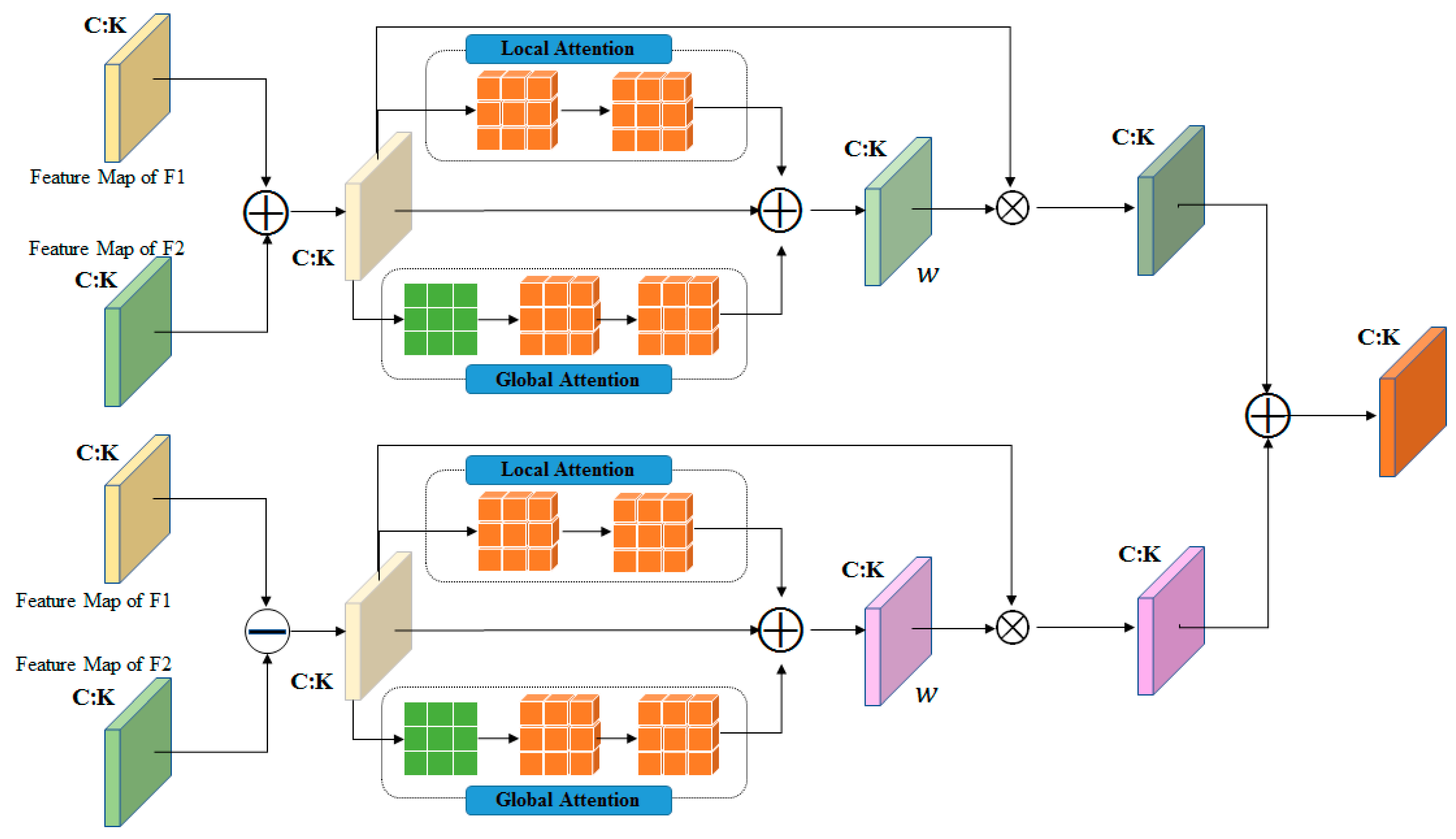
In the encoder section, we extract multi-scale bitemporal image feature maps through the Siamese network and AGFM. The FESCM allows the aggregation of feature maps at different scales. However, it is difficult to effectively represent semantic information by element addition or the channel tandem aggregation of biaxial feature maps [48]. In order to make full use of the multi-scale feature map, we designed FEM in FESCM to aggregate local and global information to compensate for the inconsistency of attentional feature fusion at different scales.

As shown in Figure 6, in the FEM section, we first add or subtract the previously obtained feature maps F1 and F2 of the two temporal images to obtain the fusion information. The local contextual information is then aggregated through the local attention module (LAM). In the local attention module, we use point-wise convolution (PWConv) to aggregate local attention information, which can be obtained as follows:

$$LAM\left(F\right)=\mathcal{B}\left({PWConv}_2\right(\delta \left(\mathcal{B}\mathcal{R}\right({PWConv}_1\left(x\right)\left)\right)\left)\right)$$

(10)

where $\mathcal{B}$ denotes batch normalization (BN), $\mathcal{R}$ denotes rectified linear unit (ReLU) activation, and $\delta$ denotes the sigmoid function.

In the global attention module (GAM), we use global average pooling (GAPool) to aggregate global context information, which can be obtained as follows:

$$GAPool\left(F\right)=\frac{1}{H\times W}{\sum }_{i=1}^H{\sum }_{j=1}^W{F}_{\left[:,i,j\right]}$$

(11)

To further enhance global information, we use GAM to capture the feature map to obtain more complete change information. The formula is as follows:

$$GAM\left(F\right)=\mathcal{B}\left({PWConv}_2\right(\delta \left(\mathcal{B}\mathcal{R}\right({PWConv}_1\left(\mathrm{G}\mathrm{A}\mathrm{P}\mathrm{o}\mathrm{o}\mathrm{l}\left(F\right)\right)\left)\right)\left)\right)$$

(12)

where $\mathcal{B}$ denotes BN, $\mathcal{R}$ denotes ReLU, and $\delta$ denotes the sigmoid function.

3.4. Loss Function

The loss function is employed to quantify the discrepancy between the output of the model and its true value and to offer recommendations for model optimization. A proper loss function must be chosen in order to make the most of the model’s training efficiency. This study uses a hybrid loss function to mitigate the impact of sample imbalance since the amount of changed pixels in the change detection domain is significantly less than the number of background pixels. The subject loss function and the edge loss function are the two fundamental components of the hybrid loss function. The expected building change results are monitored using the subject loss function. The expected edge detection results are monitored using the edge loss function. What follows is a description of the hybrid loss functions for the main body loss function and the edge loss function, which are designated by $L_{out}$ and $L_{edge}$, respectively.

$$L={\lambda }_1{L}_{out}+{\lambda }_2{L}_{edge}$$

(13)

In the task of building change detection, the number of background pixels is far greater than the number of pixels of changed buildings. During model training, the easily classified negative samples have a great impact on the optimization direction of the model. In order to solve the imbalance problem between positive and negative samples, the focal loss detection method is suggested in an effort to balance out the proportion of challenging and straightforward samples. The focal loss has the following formula:

$$L_{f_1}=\left\{\begin{array}{c} -\alpha {\left(1-y^{\prime }\right)}^{\gamma }log{y}^{\prime }, y=1\\ -\left(1-\alpha \right){\left(y^{\prime }\right)}^{\gamma }log{\left(1-y^{\prime }\right)}^{\prime }, y=0\end{array}\right.$$

(14)

where $y^{\prime }$ represents the predicted value and y represents the true ground. $\alpha$ denotes the weights of positive and negative samples. $\gamma$ denotes the focusing parameter. This paper set $\alpha =0.25$ and $\gamma =2.0$.

To minimize the difference between the predicted building edge and the true value, we use the MSE loss function for the prediction of the building edge. The MSE loss function is utilized for the average sum of squares of the discrepancies between the predicted and true values for the edge loss function. The precise formula is given below:

$$MSE=\frac{1}{m}\sum _{i=1}^m{\left({\widehat{y}}^i-y^i\right)}^2$$

(15)

where ${\widehat{y}}^i$ denotes the model prediction output result, $y^i$ denotes the true label result, and m is the total number of pixels.

4. Datasets and Experimental Implementations

4.1. Datasets

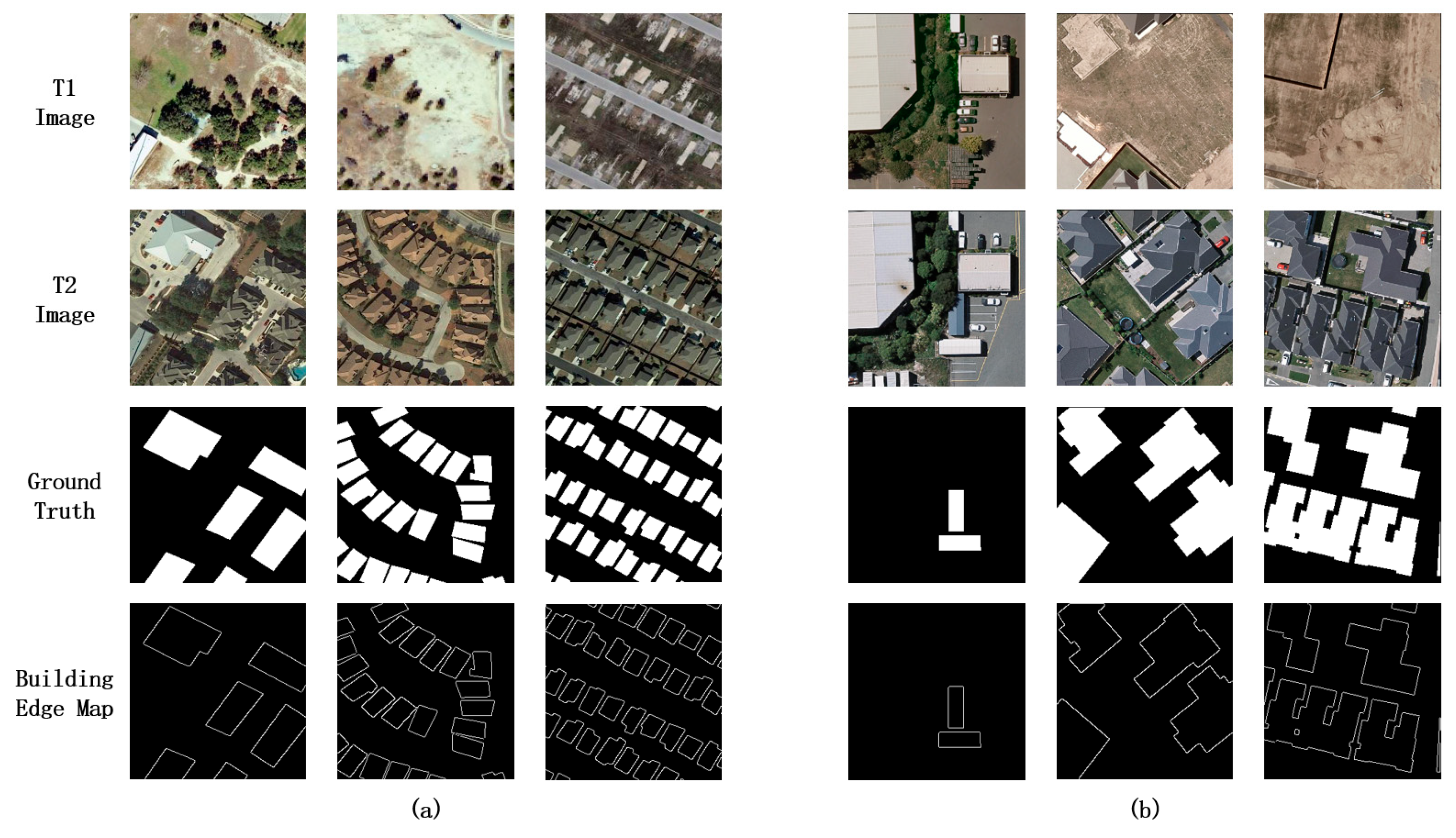
In order to verify the performance and robustness of our proposed model, we conducted comparison experiments on the WHU-CD dataset [49] and the LEVIE-CD dataset [39]. Details of the WHU-CD and LEVIR-CD datasets are shown in

Table 1. Experiment datasets.

Datasets	Data Collection	Bands	Resolution/m	Image Size	Training Set	Validation Set	Test Set
WHU-CD	Aerial Image	3	0.3	32,207 × 15,354	5460	780	1560
LEVIR-CD	Google Earth	3	0.5	1024 × 1024	7120	1024	2048

. Figure 7 presents the examples from the datasets. Based on the original dataset, we further cropped the dataset to a size of 256 × 256.

WHU-CD dataset: This dataset contains two periods of aerial images, with a size of 32,507 × 15,354. The geographic resolution of this dataset, which covers over 22,000 different buildings in Christchurch and was compiled in 2012 and 2016, is 0.2 m per pixel.

LEVIR-CD dataset: The LEVIR-CD dataset consists of 637 groups of ultrahigh-resolution Google Maps pictures with a size of 1024 × 1024 pixels. Each group of images includes the images before and after the building changes and a corresponding label. Different types of structures are covered by LEVIR-CD, including villa homes, high-rise flats, small garages, and enormous warehouses. These diachronic photos, which cover 5 to 14 years, show notable land use changes, particularly the expansion of buildings.

4.2. Comparison Methods

To verify the effectiveness of our proposed model, we selected some classical building change detection models and state-of-the-art building change detection networks for comparison, including the FC-EF [35], FC-SC [35], and FC-SD models [35], the edge-guided cyclic convolution neural network (EGRCNN) [50], and the change detection model based on the transformer (BITNet) [33]. FC-EF, FC-SC, and FC-SD are all UNet-based network models that optimize network performance by adding Siamese structures or changing hopping connections, and are classical CD models. The EGRCNN model focuses on the impact of building boundaries on network performance. The BITNet model uses transformers to model the spatial–temporal contextual information in the image to improve model accuracy.

4.3. Implementation Details

Our proposed model implementation uses the Pytorch 1.10 framework based on the Python 3.8 programming language. This study uses the Adam optimizer to train the model. The initial learning rate is 10-4, and the weight decay is 10-3. The learning rate is adjusted by observing whether the F1 score of the validation set increases within eight epochs. If no increase is observed, the learning rate is reduced by a factor of 0.05. Our proposed method is trained for 100 epochs on the LEVIR-CD dataset and WHU-CD dataset, and the network reaches a state of convergence. All training and testing experiments in the study were performed on a server equipped with an NVIDIA GeForce RTX 3090Ti GPU (with 24 GB of RAM).

4.4. Evaluation Metrics

In order to test the performance of FERA-Net in our experiments, we used the following four evaluation metrics: precision (P), recall (R), F1 score, and intersection over union (IoU). Specifically, the above evaluation metrics can be represented by the following formulas:

$$Precision=\frac{TP}{TP+FP}$$

(16)

$$Recall=\frac{TP}{TP+FN}$$

(17)

$$F1=\frac{2\times Precision\times Recall}{Precision+Recall}$$

(18)

$$IoU=\frac{TP}{TP+FP+FN}$$

(19)

where TP represents the number of pixels correctly identified as a changed building, FP represents the number of pixels incorrectly identified as a changed building, TN is the number of pixels correctly identified to have changed, and FN is the number of false negatives.

5. Results and Analysis

5.1. Results for WHU-CD

Table 2. Comparison of quantitative evaluation indicators in the WHU-CD dataset, where the best values are in bold.

Method	P (%)	R (%)	F1 (%)	IoU (%)
FC-EF [35]	83.91	79.23	81.50	68.78
FC-SC [35]	71.20	85.10	77.53	63.30
FC-SD [35]	73.36	82.87	77.83	63.70
CDNet [51]	91.75	86.89	89.62	80.60
UNet++MSOF [18]	91.96	89.40	90.66	82.92
STANet [39]	78.73	87.41	82.84	74.57
DASN [52]	88.23	84.62	86.39	76.04
SNUNet [32]	79.25	85.38	82.20	69.78
BITNet [33]	87.32	91.16	89.20	80.50
EGRCNN [50]	84.65	94.34	89.23	80.55
FERA-Net	93.51	91.47	92.48	86.01

shows the quantitative evaluation results of FERA-Net and other CD networks on the WHU-CD dataset. In addition to comparisons with the models presented in Section 4.2, we also present recent experimental data from a number of other state-of-the-art models on the WHU-CD dataset. Among them, the proposed method’s p value, F1 score, and IoU are the highest, at 93.51%, 92.52%, and 86.07%, respectively. Despite the fact that it did not achieve the highest R value, FERA-Net achieved the highest p value and F1 score. The results show that our proposed network can successfully balance network performance while concentrating more precisely on the building change area and fully characterizing the change. In particular, FERA-Net’s p value of 93.51% is much higher than that of the other change detection networks, indicating that FERA-Net is able to extract individual buildings more completely. In addition, we observed from the data that some other CD networks had large differences in p and R values, suggesting unbalanced network performance, which may have resulted in the network either failing to capture the building in its entirety or failing to identify more areas of change. The p and R values of FERA-Net are relatively close, which indicates that the network is both effective in identifying areas of building change and accurate in characterizing building edges. Regarding the recall metric, the FERA-Net does not achieve the highest score. One of the main reasons is the existence of mislabeled samples, which can be observed visually in the ground truth. As a result, FERA-Net does not classify these mislabeled regions. Thus, a higher FN value will be generated by the FERA-Net, leading to a decrease in recall.

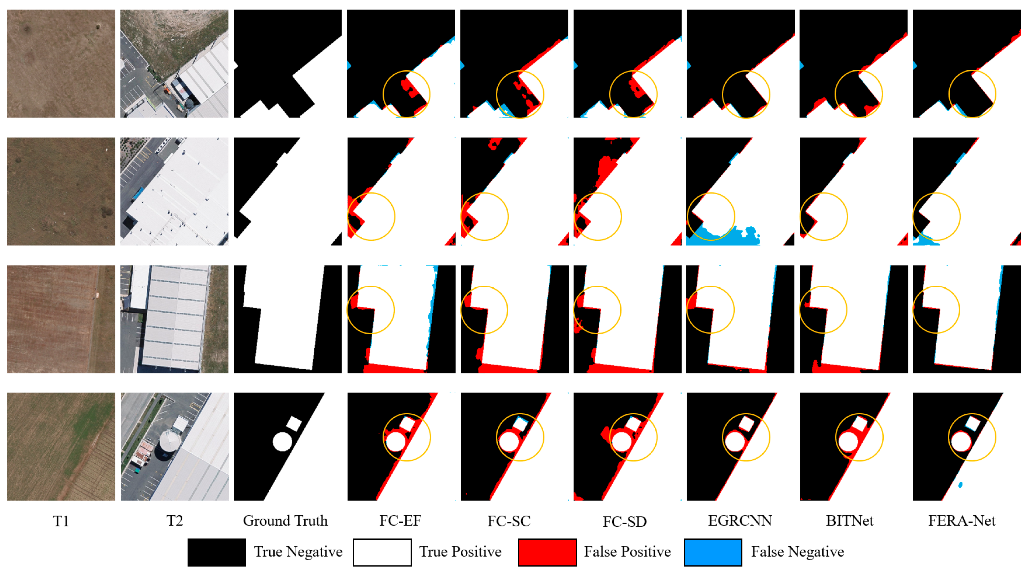
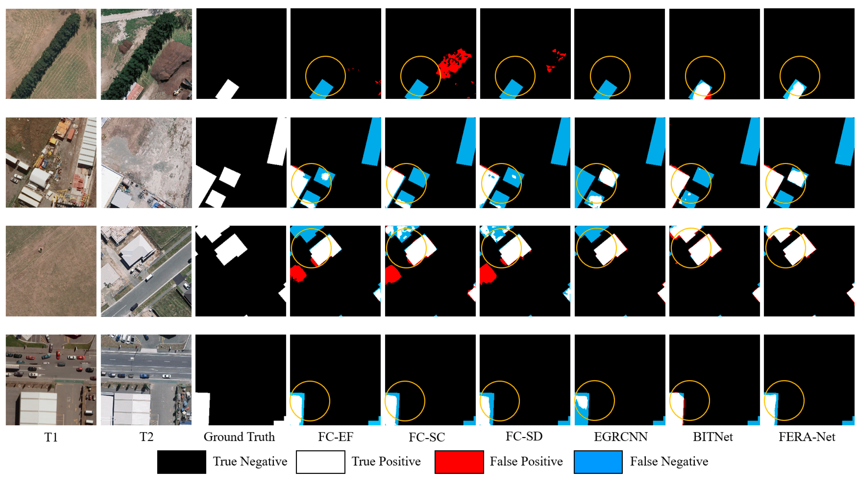
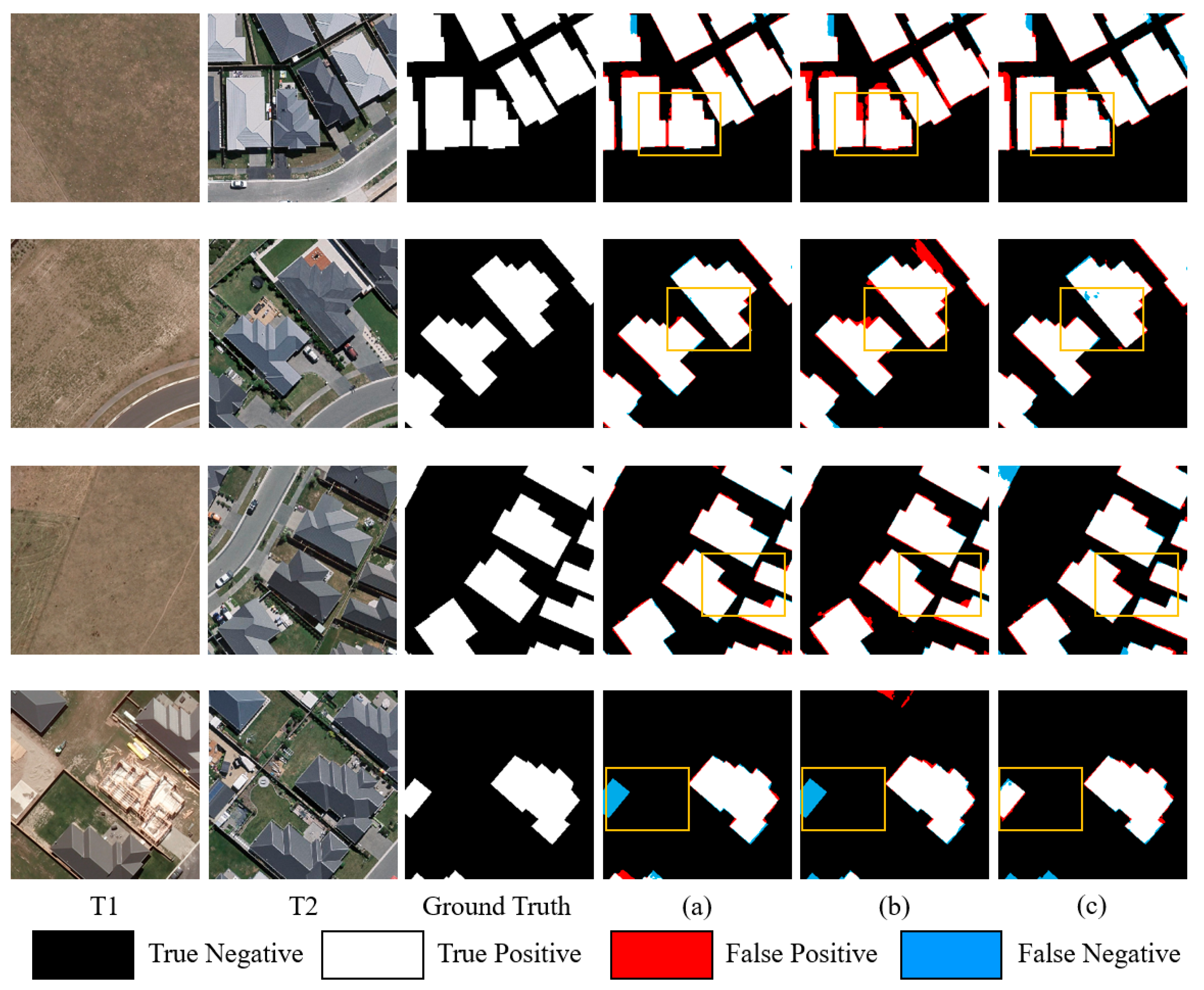
In the qualitative evaluation results, we visualized eight change detection scenarios in the WHU-CD dataset. Among them, Figure 8 shows the detection effect of FERA-Net for building boundaries. Figure 9 shows the detection of FERA-Net for building change areas in complex scenarios. In order to better represent the detection results, the TP, FP, TN, and FN values are shown in different colors, and the areas where the different networks have significant differences are further highlighted by yellow circles. From the results shown in Figure 8 and Figure 9, the following can be seen:

(1)

Accurately describing the shape structures of buildings with ambiguous edges is a great challenge. As shown in Figure 8, FERA-Net can precisely describe the boundary information of the region and segment the border of the changing area more finely. It can also effectively reduce the edge noise of moving buildings.

(2)

The interference from various manufactured things, such as roads, containers, and cars, might result in the inaccurate identification of change regions in complicated contexts with building change areas. Figure 9 illustrates that FERA-Net can more precisely capture the building regions of interest.

5.2. Results for LEVIR-CD

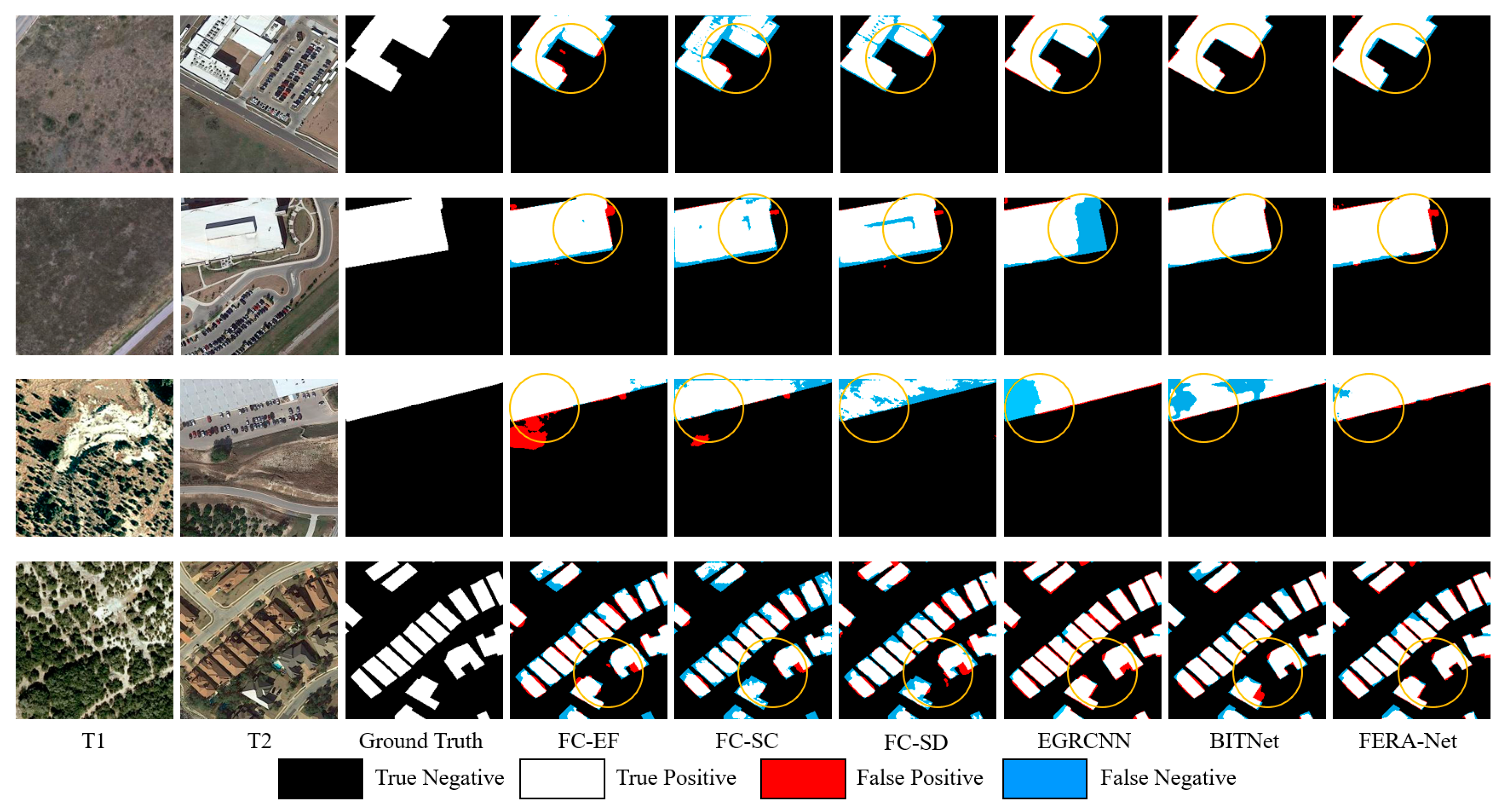
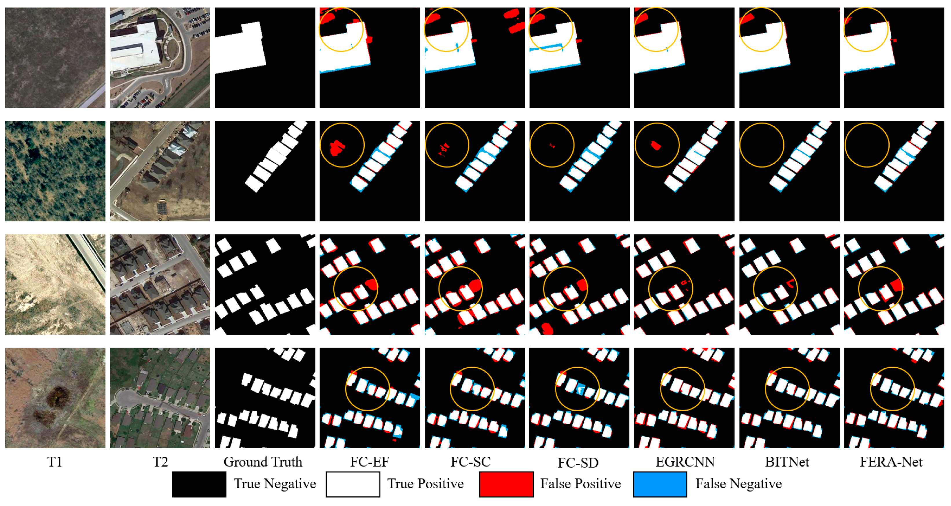
We also evaluated the performance of FERA-Net on the LEVIR-CD dataset to validate the robustness of the model. In

Table 3. Comparison of quantitative evaluation indicators in the LEVIR-CD dataset, where the best values are in bold.

Method	P (%)	R (%)	F1 (%)	IoU (%)
FC-EF [35]	83.97	84.01	83.99	72.40
FC-SC [35]	86.05	80.19	83.01	70.96
FC-SD [35]	88.57	83.60	86.01	75.46
STANet [39]	85.93	81.57	83.68	74.64
SNUNet [32]	90.32	86.22	88.23	78.94
BITNet [33]	91.41	85.53	88.37	79.17
EGRCNN [50]	88.11	90.39	89.24	80.57
CDNet [51]	90.50	84.60	87.50	-
HDFNet [53]	87.54	89.38	88.13	-
HRTNet [54]	85.43	91.77	88.48	-
FERA-Net	91.57	87.68	89.58	80.27

, the results of the quantitative evaluation of FERA-Net with other change detection networks are presented. From the quantitative evaluation results, we can see that FERA-Net achieved the highest scores on the LEVIR-CD dataset for both evaluation indicators, p value and F1 score, which is consistent with the results on the WHU-CD dataset. It can be seen from the results that FERA-Net achieves the highest p value and F1 score of 91.57% and 89.58%, respectively. Although our proposed model’s IoU score for the LEVIR-CD dataset is not as high as on the WHU-CD dataset, it is still the second highest among all models in the experiment. Furthermore, our FERA-Net can improve the p value, F1 score, and IoU, demonstrating our suggested network’s ability to balance the p and R values. FERA-Net can precisely identify the building change regions in the remote sensing images and also fully characterize all of the specific properties of the regions.

Figure 10 and Figure 11 show the test results of the CD networks. FERA-Net can produce the most visually accurate change detection findings. The detection maps maintain higher internal compactness with more complete building contours. As can be seen from the visualization in Figure 10, FERA-Net is able to identify building edges more accurately for multi-scale buildings. We believe that the high-frequency feature module designed in the network is extremely useful for this result. At the same time, as seen from the results in Figure 11, FERA-Net can reduce interference in remote sensing images and more precisely pinpoint the locations of building changes.

5.3. Ablation Study

In order to verify the validity of the key modules, we conducted a series of ablation experiments on WHU-CD datasets in which several FERA-Net network modules were deleted. The effects of various encoders and connection methods on the outcomes of building change detection are specifically covered in this section. The encoder candidates cover CNN and AGFM encoders, and for comparison with other connection methods, full-scale skip connection module (FSCM) and FESCM are chosen. Additionally, our basic model combines the Siam network and UNet3+ models.

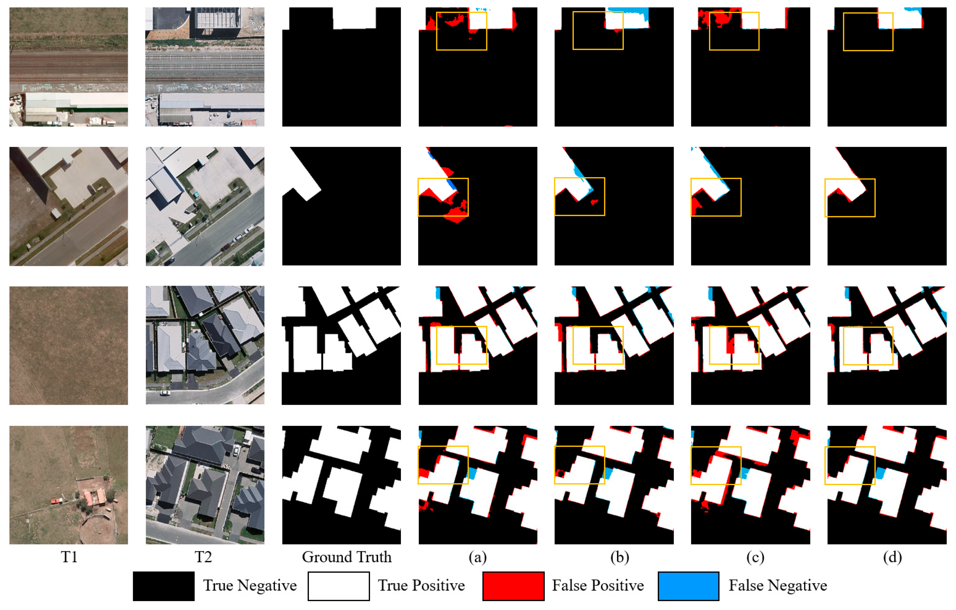
The quantitative results are listed in

Table 4. Quantitative evaluation metrics for ablation experiments on the WHU-CD dataset, where the best values are in bold.

ID	Encoder Method	Connection Method	P (%)	R (%)	F1 (%)	IoU (%)
(a)	CNN	FSCM	89.12	88.22	88.67	79.64
(b)	CNN	FESCM	88.17	90.50	90.76	83.08
(c)	AGFM	FSCM	92.20	88.90	90.53	82.69
(d)	AGFM	FESCM	92.44	91.31	91.88	84.97

. Row (a,c) and row (b,d) verify the validity of the AGFM module. Row (a,b) and row (c,d) verify the validity of the FESCM module. The results reveal that utilizing the AGFM as the model’s encoder can significantly increase the model’s detection accuracy compared with using the CNN module. In comparison to the CNN module, utilizing the AGFM module increases the p value, F1 score, and IoU, which indicates that using the AGFM module is effective for building integrity detection. The experiment with FESCM shows that this module is more effective than the feature-enhanced skip connection module: p value, R value, F1 score, and IoU increase by 0.24%, 4.41%, 1.35%, and 2.28%, respectively. These improvements indicate that the FESCM can capture more information on building change areas and reduces the number of missed detections for changing buildings.

Figure 12 shows the ablation experiment result. Dual-time images and the labeled changes are denoted by (a–c). The change detection results from the combinations of the modules in Table 4 are denoted by (d–g). It can be observed that the network can capture the building change area more precisely when it utilizes the AGFM module. It can also minimize boundary noise and characterize the building boundary in more detail. The quantity of missed and false detections gradually decreased in the findings obtained using FESCM.

6. Discussion

6.1. Effectiveness of the AGFM

In order to analyze the effectiveness of the attention mechanism in the task of building change detection, we examined the performance of a conventional CNN encoder, CBAM encoder (a conventional spatial attention and channel attention module), and AGFM encoder. In this instance, we employed a Siamese network structure, focal loss, and UNet3+ as the baseline.

Table 5. Effectiveness of the AGFM, where the best values are in bold.

ID	Encoder Method	Connection Method	P (%)	R (%)	F1 (%)	IoU (%)
(a)	CNN	FSCM	89.12	88.22	88.67	79.64
(b)	CBAM	FSCM	85.31	91.84	88.46	79.30
(c)	AGFM	FSCM	92.20	88.90	90.53	82.69

displays the quantitative evaluation results: by using the AGFM module, the p value is 3.08% higher than when using the CNN encoder and 6.89% higher than when using the CBAM encoder. This indicates that the AGFM encoder can improve the model in learning the overall building characteristics. Using the AGFM module, the R value is 0.78% higher than the CNN encoder but 2.94% lower than the CBAM encoder. We believe the reason for this is that the AGFM module is more concerned with representing detailed building features but is not the best for extracting changing building areas. Additionally, the AGFM encoder significantly improves the F1 score and IoU assessment metrics by 90.53% and 82.69%, respectively. Overall, the building change detection job benefits more from the AGFM encoder when compared with the CNN encoder and conventional attention encoder.

Figure 13 displays the CD result on the WHU-CD dataset using the CNN, CBAM, and AGFM encoders. According to the figure, the AGFM encoder is superior to the CNN and CBAM encoders in its ability to characterize the main portion of the building and the boundary of the changing building. The other two encoders are susceptible to the building connection part and image classification accuracy in dense building areas, but the AGFM can accurately characterize the building’s edge. When describing local information, the AGFM encoder is not compared with the CBAM encoder, which can explain the R value portion of Table 5.

Considering the good performance of attention mechanisms in the building change detection task in previous studies, we conducted validation experiments on the WHU-CD dataset for the residual spatial attention feature extraction stage (RSAS) and high-frequency residual channel attention enhancement stage (FRCS) in the AGFM module. We aimed to verify the performance of the high-frequency features of the images and attention mechanism for further confirming the mechanism of the AGFM module in FERA-Net in the building CD task.

According to the quantitative analysis in

Table 6. Effectiveness of RSAS and FRCS, where the best values are in bold.

ID	Encoder Method	Connection Method	P (%)	R (%)	F1 (%)	IoU (%)
(a)	RSAS	FESCM	89.53	90.67	90.10	81.98
(b)	FRCS	FESCM	91.75	88.64	90.17	82.10
(c)	RSAS + FRCS	FESCM	92.20	88.90	90.53	82.69

, adding the FRCS module to the RSAS module can significantly improve the p value of the change detection task, which suggests that we can increase the quality of the building edge information and improve the model detection accuracy by introducing high-frequency features into the transformation detection task.

6.2. Effectiveness of the FESCM

Since the encoder downsampling process will lose spatial information in the encoder–decoder network structure, it is important to compensate for the lost spatial information in the decoder part by skipping the connection. However, the skip connection used in UNet only collects data from the feature map of the same level. This skip connection between sibling feature maps allows the network to create a semantic gap between the decoder’s higher-level and lower-level feature maps. The lower-level feature maps in UNet mainly acquire fine-grained detailed features (capturing rich spatial information), and the higher-level feature maps mainly acquire coarse-grained semantic features (capturing location information). In contrast, the FERA-Net utilized in this study employs FESCM, which maximizes the utilization of full-scale feature maps and enhances segmentation accuracy by fusing spatial and semantic information from feature maps at different scales.

We designed three additional experiments to verify the efficacy of FESCM described above for the building change detection task. Six comparative experiments were designed to verify the impact of skip connection (SC) in UNet and full-scale skip connection (FSSC) in UNet3+ and the FESCM. As shown in

Table 7. Effectiveness of the FESCM, where the best values are in bold.

ID	Encoder Method	Connection Method	P (%)	R (%)	F1 (%)	IoU (%)
(a)	CNN	SC	83.82	90.63	87.09	77.14
(b)	CNN	FSSC	89.12	88.22	88.67	79.64
(c)	CNN	FESCM	88.17	90.50	90.76	83.08
(d)	AGFM	SC	88.83	92.46	90.61	82.84
(e)	AGFM	FSSC	92.20	88.90	90.53	82.69
(f)	AGFM	FESCM	92.44	91.31	91.88	84.97

, the most notable improvements are 5.3% in the p value, 1.56% in the F1 score, and 2.50% in the IoU, but the R value decreased by 2.41%.

Figure 14 shows the visualization results of the experiments: the UNet3+ network with full-scale skip links can describe the change building information more comprehensively than the UNet network, which proves the important role of full-scale skip links in the change detection task. The FESCM obtained the best experimental results, verifying that the FESCM outperforms the FSSC in the fusion of detailed information in low-level feature maps and semantic information in high-level feature maps. This explains the increase in p value and the decrease in R value in Table 6, as it also results in the decoder part of the model incorporating some interference information, which weakens the model’s identification of areas of building change. However, in general, adding full-scale skip connections to the building change detection problem helps to improve the model’s overall detection performance.

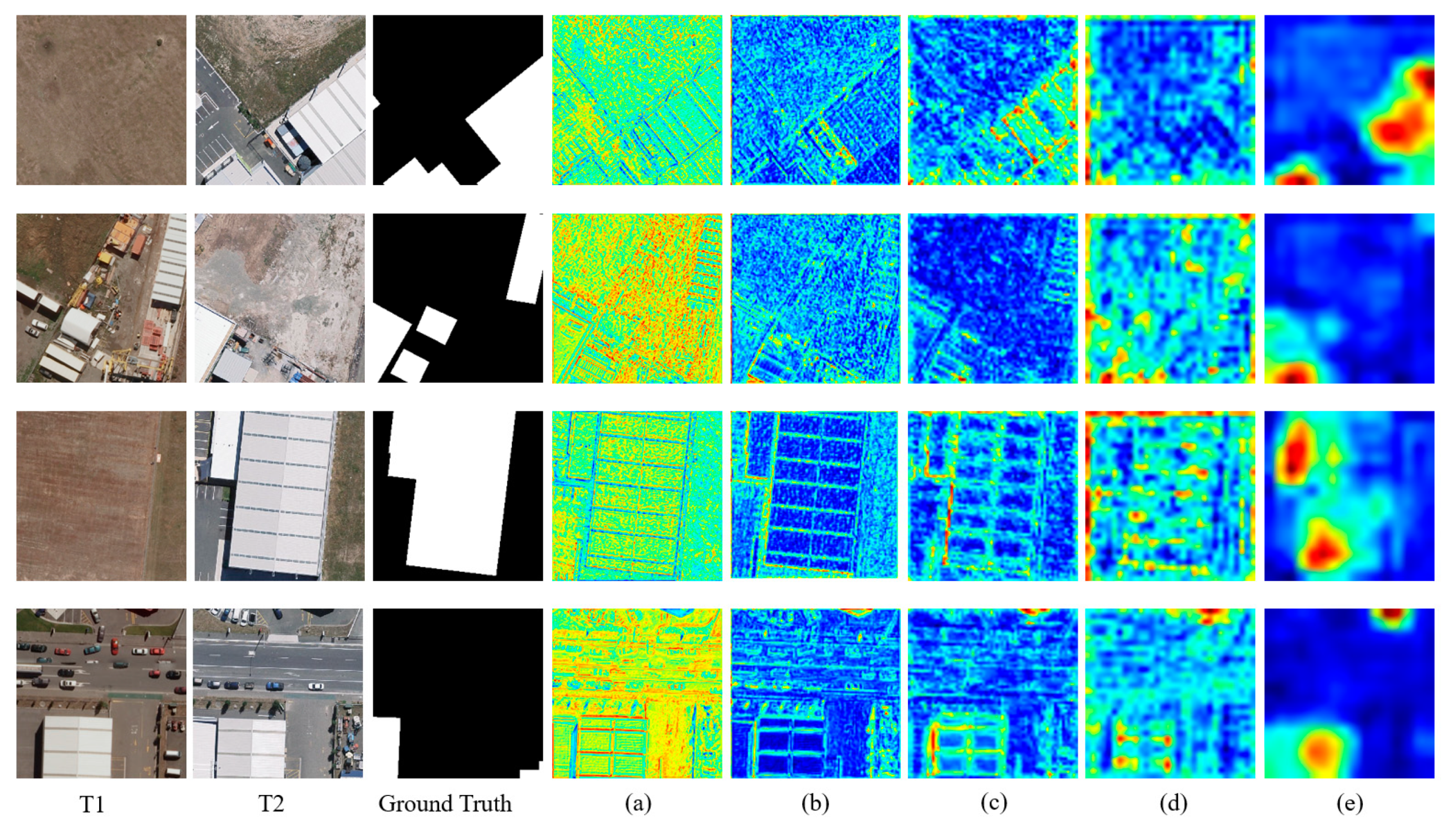
In addition to the quantitative analysis of the evaluation indicators above, we also visualized the five layers of feature maps in the model, as shown in Figure 15. From the feature maps, we can see that, with the AGFM and FEM, the model focuses on the details of the remote sensing images in the first-, second-, and third-layer feature maps, especially the edges of the buildings, while the last two layers capture the spatial information and focus on the building change areas. The feasibility of the FESCM module was also verified from the visualization results: the different levels of feature maps contain different information, and the FESCM module provides the model’s decoder with more comprehensive information about the buildings, which helps to better identify areas of change.

6.3. Effectiveness of the Hybrid Loss Function

At the final layer of the encoder, FERA-Net performs edge extraction to optimize edge supervision and model constraints for improved learning of boundary information. This part focuses on the edge loss’s effect on the detection process results. The main body function and the edge loss function constitute the loss function in this study. $L_{out}$ stands for the main body function and $L_{edge}$ stands for the edge loss function.

Table 8. Effectiveness of hybrid loss function, where the best values are in bold.

ID	Body Loss	Edge Loss	P (%)	R (%)	F1 (%)	IoU (%)
(a)	$L_{out}$	None	92.44	91.31	91.88	84.97
(b)	${0.9\times L}_{out}$	$0.1\times L_{edge}$	92.96	91.04	91.99	85.16
(c)	$0.8\times L_{out}$	$0.2\times L_{edge}$	93.51	91.47	92.48	86.01
(d)	$0.7\times L_{out}$	$0.3\times L_{edge}$	90.29	91.16	90.72	83.02

shows the impact of our different weighting designs in the hybrid loss function on the performance of the model. As shown in the quantitative evaluation results in Table 8, the model’s overall performance was improved by using the hybrid loss function. In particular, the best performance improvement was achieved when the weight of the edge loss function was set to 0.2, where the P value, R value, F1 score, and IoU improved by 1.07%, 0.16%, 0.60%, and 1.04%, respectively. This suggests that the edge loss function $L_{edge}$ can improve the network’s ability of extracting boundary information. With the function, the model can more precisely characterize the building border, which enhances the effectiveness of network detection.

7. Conclusions

This paper proposes a new deep learning network applied to the change detection task named FERA-Net. FERA-Net is a typical encoder–decoder architecture. In the encoder section, we designed the AGFM to extract multi-level feature maps. In the decoder part, we fused the multi-scale feature maps with an FESCM. The AGFM uses a spatial attention mechanism to capture areas of building change and a channel attention mechanism to fuse high-frequency features extracted by the omnidirectional Sobel operator into the feature map. To maximize the use of full-size feature maps and to improve change detection accuracy, we use the FESCM to enhance the global and local information in the building change feature maps and link low-level detailed information with high-level semantic information. In addition, we designed hybrid loss functions to monitor building edges by means of changing the building boundaries extracted at the last layer of the decoder. Compared with other change detection methods, our method can utilize the local and global information of the feature maps and recognize multi-scale feature buildings in highly fractioned remote sensing images. We validated the performance of FERA-Net on the WHU-CD and LEVIR-CD datasets. From the quantitative and qualitative evaluation results, we can see that FERA-Net performs excellently on the two datasets. In the evaluation of quantitative metrics, we compared FERA-Net with classical change detection networks and state-of-the-art change detection networks, achieving the highest p value and F1 score. In the evaluation of qualitative visualization results, FREA-Net can effectively extract building change areas in complex ground environments, while accurately identifying building boundaries and maintaining boundary integrity. However, FERA-Net requires a large number of samples to learn in order to achieve good classification results. The performance of the current supervised building change detection network encounters a bottleneck, and the implementation of semi-supervised change detection based on the FERA-Net network will be the focus of future work.

References

1. Zhu, Q.; Guo, X.; Deng, W.; Shi, S.; Guan, Q.; Zhong, Y.; Zhang, L.; Li, D. Land-Use/Land-Cover Change Detection Based on a Siamese Global Learning Framework for High Spatial Resolution Remote Sensing Imagery. ISPRS J. Photogramm. Remote Sens. 2022, 184, 63–78. [Google Scholar] [CrossRef]
2. Song, K.; Jiang, J. AGCDetNet:An Attention-Guided Network for Building Change Detection in High-Resolution Remote Sensing Images. IEEE J. Sel. Top. Appl. Earth Obs. Remote Sens. 2021, 14, 4816–4831. [Google Scholar] [CrossRef]
3. Jensen, J.R.; Im, J. Remote Sensing Change Detection in Urban Environments. In Geo-Spatial Technologies in Urban Environments: Policy, Practice, and Pixels; Jensen, R.R., Gatrell, J.D., McLean, D., Eds.; Springer: Berlin/Heidelberg, Germany, 2007; pp. 7–31. ISBN 978-3-540-69417-5. [Google Scholar]
4. Singh, A. Review Article Digital Change Detection Techniques Using Remotely-Sensed Data. Int. J. Remote Sens. 1989, 10, 989–1003. [Google Scholar] [CrossRef] [Green Version]
5. Bruzzone, L.; Bovolo, F. A Novel Framework for the Design of Change-Detection Systems for Very-High-Resolution Remote Sensing Images. Proc. IEEE 2013, 101, 609–630. [Google Scholar] [CrossRef]
6. Hussain, M.; Chen, D.; Cheng, A.; Wei, H.; Stanley, D. Change Detection from Remotely Sensed Images: From Pixel-Based to Object-Based Approaches. ISPRS J. Photogramm. Remote Sens. 2013, 80, 91–106. [Google Scholar] [CrossRef]
7. Jiang, H.; Peng, M.; Zhong, Y.; Xie, H.; Hao, Z.; Lin, J.; Ma, X.; Hu, X. A Survey on Deep Learning-Based Change Detection from High-Resolution Remote Sensing Images. Remote Sens. 2022, 31, 1552. [Google Scholar] [CrossRef]
8. Quarmby, N.A.; Cushnie, J.L. Monitoring Urban Land Cover Changes at the Urban Fringe from SPOT HRV Imagery in South-East England. Int. J. Remote Sens. 1989, 10, 953–963. [Google Scholar] [CrossRef]
9. Zanotta, D.C.; Haertel, V. Gradual Land Cover Change Detection Based on Multitemporal Fraction Images. Pattern Recognit. 2012, 45, 2927–2937. [Google Scholar] [CrossRef]
10. Deng, J.S.; Wang, K.; Deng, Y.H.; Qi, G.J. PCA-based Land-use Change Detection and Analysis Using Multitemporal and Multisensor Satellite Data. Int. J. Remote Sens. 2008, 29, 4823–4838. [Google Scholar] [CrossRef]
11. Ertürk, A.; Iordache, M.-D.; Plaza, A. Sparse Unmixing-Based Change Detection for Multitemporal Hyperspectral Images. IEEE J. Sel. Top. Appl. Earth Obs. Remote Sens. 2016, 9, 708–719. [Google Scholar] [CrossRef]
12. Bruzzone, L.; Cossu, R.; Vernazza, G. Detection of Land-Cover Transitions by Combining Multidate Classifiers. Pattern Recognit. Lett. 2004, 25, 1491–1500. [Google Scholar] [CrossRef]
13. Bruzzone, L.; Prieto, D.F. Automatic Analysis of the Difference Image for Unsupervised Change Detection. IEEE Trans. Geosci. Remote Sens. 2000, 38, 1171–1182. [Google Scholar] [CrossRef] [Green Version]
14. Habib, T.; Inglada, J.; Mercier, G.; Chanussot, J. Support Vector Reduction in SVM Algorithm for Abrupt Change Detection in Remote Sensing. IEEE Geosci. Remote Sens. Lett. 2009, 6, 606–610. [Google Scholar] [CrossRef]
15. Quispe, D.A.J.; Sulla-Torres, J. Automatic Building Change Detection on Aerial Images Using Convolutional Neural Networks and Handcrafted Features. Int. J. Adv. Comput. Sci. Appl. 2020, 11, 679–684. [Google Scholar] [CrossRef]
16. Roy, M.; Ghosh, S.; Ghosh, A. A Novel Approach for Change Detection of Remotely Sensed Images Using Semi-Supervised Multiple Classifier System. Inf. Sci. 2014, 269, 35–47. [Google Scholar] [CrossRef]
17. Bontemps, S.; Bogaert, P.; Titeux, N.; Defourny, P. An Object-Based Change Detection Method Accounting for Temporal Dependences in Time Series with Medium to Coarse Spatial Resolution. Remote Sens. Environ. 2008, 112, 3181–3191. [Google Scholar] [CrossRef]
18. Peng, D.; Zhang, Y.; Guan, H. End-to-End Change Detection for High Resolution Satellite Images Using Improved UNet++. Remote Sens. 2019, 11, 1382. [Google Scholar] [CrossRef] [Green Version]
19. Ma, J.; Lu, D.; Li, Y.; Shi, G. CLHF-Net: A Channel-Level Hierarchical Feature Fusion Network for Remote Sensing Image Change Detection. Symmetry 2022, 14, 1138. [Google Scholar] [CrossRef]
20. Addink, E.A.; Van Coillie, F.M.B.; De Jong, S.M. Introduction to the GEOBIA 2010 Special Issue: From Pixels to Geographic Objects in Remote Sensing Image Analysis. Int. J. Appl. Earth Obs. Geoinf. 2012, 15, 1–6. [Google Scholar] [CrossRef]
21. Huang, X.J.; Xie, Y.W.; Wei, J.J.; Fu, M.; Lv, L.L.; Zhang, L.L. Automatic Recognition of Desertification Information Based on the Pattern of Change Detection-CART Decision Tree. J. Catastrophol. 2017, 32, 36–42. [Google Scholar]
22. Javed, A.; Jung, S.; Lee, W.H.; Han, Y. Object-Based Building Change Detection by Fusing Pixel-Level Change Detection Results Generated from Morphological Building Index. Remote Sens. 2020, 12, 2952. [Google Scholar] [CrossRef]
23. Lv, P.; Zhong, Y.; Zhao, J.; Zhang, L. Unsupervised Change Detection Based on Hybrid Conditional Random Field Model for High Spatial Resolution Remote Sensing Imagery. IEEE Trans. Geosci. Remote Sens. 2018, 56, 4002–4015. [Google Scholar] [CrossRef]
24. Sun, X.; Wang, P.; Wang, C.; Liu, Y.; Fu, K. PBNet: Part-Based Convolutional Neural Network for Complex Composite Object Detection in Remote Sensing Imagery. ISPRS J. Photogramm. Remote Sens. 2021, 173, 50–65. [Google Scholar] [CrossRef]
25. Wang, Z.; Zhang, Y.; Luo, L.; Wang, N. TransCD: Scene Change Detection via Transformer-Based Architecture. Opt. Express 2021, 29, 41409–41427. [Google Scholar] [CrossRef]
26. Liu, G.; Li, L.; Jiao, L.; Dong, Y.; Li, X. Stacked Fisher Autoencoder for SAR Change Detection. Pattern Recognit. 2019, 96, 106971. [Google Scholar] [CrossRef]
27. Chen, H.; Wu, C.; Du, B.; Zhang, L.; Wang, L. Change Detection in Multisource VHR Images via Deep Siamese Convolutional Multiple-Layers Recurrent Neural Network. IEEE Trans. Geosci. Remote Sens. 2020, 58, 2848–2864. [Google Scholar] [CrossRef]
28. Liu, R.; Cheng, Z.; Zhang, L.; Li, J. Remote Sensing Image Change Detection Based on Information Transmission and Attention Mechanism. IEEE Access 2019, 7, 156349–156359. [Google Scholar] [CrossRef]
29. Lyu, H.; Lu, H.; Mou, L. Learning a Transferable Change Rule from a Recurrent Neural Network for Land Cover Change Detection. Remote Sens. 2016, 8, 506. [Google Scholar] [CrossRef] [Green Version]
30. Jiang, F.; Gong, M.; Zhan, T.; Fan, X. A Semisupervised GAN-Based Multiple Change Detection Framework in Multi-Spectral Images. IEEE Geosci. Remote Sens. Lett. 2020, 17, 1223–1227. [Google Scholar] [CrossRef]
31. Zhao, W.; Mou, L.; Chen, J.; Bo, Y.; Emery, W.J. Incorporating Metric Learning and Adversarial Network for Seasonal Invariant Change Detection. IEEE Trans. Geosci. Remote Sens. 2020, 58, 2720–2731. [Google Scholar] [CrossRef]
32. Fang, S.; Li, K.; Shao, J.; Li, Z. SNUNet-CD: A Densely Connected Siamese Network for Change Detection of VHR Images. IEEE Geosci. Remote Sens. Lett. 2022, 19, 1–5. [Google Scholar] [CrossRef]
33. Chen, H.; Qi, Z.; Shi, Z. Remote Sensing Image Change Detection with Transformers. IEEE Trans. Geosci. Remote Sens. 2022, 60, 1–14. [Google Scholar] [CrossRef]
34. Li, Z.; Yan, C.; Sun, Y.; Xin, Q. A Densely Attentive Refinement Network for Change Detection Based on Very-High-Resolution Bitemporal Remote Sensing Images. IEEE Trans. Geosci. Remote Sens. 2022, 60, 1–18. [Google Scholar] [CrossRef]
35. Caye Daudt, R.; Le Saux, B.; Boulch, A. Fully Convolutional Siamese Networks for Change Detection. In Proceedings of the 2018 25th IEEE International Conference on Image Processing (ICIP), Athens, Greece, 7–10 October 2018; pp. 4063–4067. [Google Scholar]
36. Zhang, C.; Yue, P.; Tapete, D.; Jiang, L.; Shangguan, B.; Huang, L.; Liu, G. A Deeply Supervised Image Fusion Network for Change Detection in High Resolution Bi-Temporal Remote Sensing Images. ISPRS J. Photogramm. Remote Sens. 2020, 166, 183–200. [Google Scholar] [CrossRef]
37. Tan, K.; Zhang, Y.; Wang, X.; Chen, Y. Object-Based Change Detection Using Multiple Classifiers and Multi-Scale Uncertainty Analysis. Remote Sens. 2019, 11, 359. [Google Scholar] [CrossRef] [Green Version]
38. Zhang, J.; Pan, B.; Zhang, Y.; Liu, Z.; Zheng, X. Building Change Detection in Remote Sensing Images Based on Dual Multi-Scale Attention. Remote Sens. 2022, 14, 5405. [Google Scholar] [CrossRef]
39. Chen, H.; Shi, Z. A Spatial-Temporal Attention-Based Method and a New Dataset for Remote Sensing Image Change Detection. Remote Sens. 2020, 12, 1662. [Google Scholar] [CrossRef]
40. Ji, S.; Shen, Y.; Lu, M.; Zhang, Y. Building Instance Change Detection from Large-Scale Aerial Images Using Convolutional Neural Networks and Simulated Samples. Remote Sens. 2019, 11, 1343. [Google Scholar] [CrossRef] [Green Version]
41. Peng, D.; Bruzzone, L.; Zhang, Y.; Guan, H.; Ding, H.; Huang, X. SemiCDNet: A Semisupervised Convolutional Neural Network for Change Detection in High Resolution Remote-Sensing Images. IEEE Trans. Geosci. Remote Sens. 2021, 59, 5891–5906. [Google Scholar] [CrossRef]
42. Zhang, L.; Hu, X.; Zhang, M.; Shu, Z.; Zhou, H. Object-Level Change Detection with a Dual Correlation Attention-Guided Detector. ISPRS J. Photogramm. Remote Sens. 2021, 177, 147–160. [Google Scholar] [CrossRef]
43. Chen, J.; Yuan, Z.; Peng, J.; Chen, L.; Huang, H.; Zhu, J.; Liu, Y.; Li, H. DASNet: Dual Attentive Fully Convolutional Siamese Networks for Change Detection of High Resolution Satellite Images. IEEE J. Sel. Top. Appl. Earth Obs. Remote Sens. 2021, 14, 1194–1206. [Google Scholar] [CrossRef]
44. Ma, J.; Shi, G.; Li, Y.; Zhao, Z. MAFF-Net: Multi-Attention Guided Feature Fusion Network for Change Detection in Remote Sensing Images. Sensors 2022, 22, 888. [Google Scholar] [CrossRef] [PubMed]
45. Chen, J.; Fan, J.; Zhang, M.; Zhou, Y.; Shen, C. MSF-Net: A Multiscale Supervised Fusion Network for Building Change Detection in High-Resolution Remote Sensing Images. IEEE Access 2022, 10, 30925–30938. [Google Scholar] [CrossRef]
46. Zheng, H.; Gong, M.; Liu, T.; Jiang, F.; Zhan, T.; Lu, D.; Zhang, M. HFA-Net: High Frequency Attention Siamese Network for Building Change Detection in VHR Remote Sensing Images. Pattern Recognit. 2022, 129, 108717. [Google Scholar] [CrossRef]
47. Wang, F.; Jiang, M.; Qian, C.; Yang, S.; Li, C.; Zhang, H.; Wang, X.; Tang, X. Residual Attention Network for Image Classification. In Proceedings of the 2017 IEEE Conference on Computer Vision and Pattern Recognition (CVPR), Honolulu, HI, USA, 21–26 July 2017; pp. 6450–6458. [Google Scholar]
48. Chen, Z.; Zhou, Y.; Wang, B.; Xu, X.; He, N.; Jin, S.; Jin, S. EGDE-Net: A Building Change Detection Method for High-Resolution Remote Sensing Imagery Based on Edge Guidance and Differential Enhancement. ISPRS J. Photogramm. Remote Sens. 2022, 191, 203–222. [Google Scholar] [CrossRef]
49. Ji, S.; Wei, S.; Lu, M. Fully Convolutional Networks for Multisource Building Extraction From an Open Aerial and Satellite Imagery Data Set. IEEE Trans. Geosci. Remote Sens. 2019, 57, 574–586. [Google Scholar] [CrossRef]
50. Bai, B.; Fu, W.; Lu, T.; Li, S. Edge-Guided Recurrent Convolutional Neural Network for Multitemporal Remote Sensing Image Building Change Detection. IEEE Trans. Geosci. Remote Sens. 2022, 60, 1–13. [Google Scholar] [CrossRef]
51. Alcantarilla, P.F.; Stent, S.; Ros, G.; Arroyo, R.; Gherardi, R. Street-View Change Detection with Deconvolutional Networks. Auton Robot 2018, 42, 1301–1322. [Google Scholar] [CrossRef]
52. Peng, X.; Zhong, R.; Li, Z.; Li, Q. Optical Remote Sensing Image Change Detection Based on Attention Mechanism and Image Difference. IEEE Trans. Geosci. Remote Sens. 2021, 59, 7296–7307. [Google Scholar] [CrossRef]
53. Zhang, Y.; Fu, L.; Li, Y.; Zhang, Y. HDFNet: Hierarchical Dynamic Fusion Network for Change Detection in Optical Aerial Images. Remote Sens. 2021, 13, 1440. [Google Scholar] [CrossRef]
54. Hou, X.; Bai, Y.; Li, Y.; Shang, C.; Shen, Q. High-Resolution Triplet Network with Dynamic Multiscale Feature for Change Detection on Satellite Images. ISPRS J. Photogramm. Remote Sens. 2021, 177, 103–115. [Google Scholar] [CrossRef]
Figure 1. Structure of the FERA-Net. FERA-Net comprises the encoder part and decoder part. The encoding part consists of five attention-guided high-frequency feature extraction modules with dual branches. The decoding part consists of a feature-enhanced skip connection module.
Remotesensing 15 00395 g001
Figure 2. Illustration of Attention-Guided High-Frequency Feature Extraction Module.
Remotesensing 15 00395 g002
Figure 3. Illustration of Residual Spatial Attention Feature Extraction Stage.
Remotesensing 15 00395 g003
Figure 4. Illustration of Residual Channel Attention High-Frequency Feature Enhancement Stage.
Remotesensing 15 00395 g004
Figure 5. Feature-enhanced skip connection module.
Remotesensing 15 00395 g005
Figure 6. Feature Enhancement Module.
Remotesensing 15 00395 g006
Figure 7. Sample images from the LEVIR-CD dataset (a) and the WHU-CD dataset (b). The first and second rows represent the remote sensing data for the dual-time images. The third row represents the change in the building ground truth. The fourth row represents the building edges extracted from the third row by the Canny edge detection algorithm.
Remotesensing 15 00395 g007
Figure 8. Visual comparison of building edge extraction results in the WHU-CD dataset.
Remotesensing 15 00395 g008
Figure 9. Visualization comparison of results in complex environments in the WHU-CD dataset.
Remotesensing 15 00395 g009
Figure 10. Visual comparison of building edge extraction results in the LEVIR-CD dataset.
Remotesensing 15 00395 g010
Figure 11. Visualization comparison of results in complex environments in the LEVIR-CD dataset.
Remotesensing 15 00395 g011
Figure 12. Visualization of ablation experiments on the WHU-CD dataset. (a) “CNN + FSCM”. (b) “CNN + FESCM”. (c) “AGFM + FSCM”. (d) “AGFM + FESCM”.
Remotesensing 15 00395 g012
Figure 13. Effectiveness of the AGFM. (a) “CNN + FSCM”. (b) “CBAM + FESCM”. (c) “AGFM + FSCM”.
Remotesensing 15 00395 g013
Figure 14. Effectiveness of the FESCM. (a) “CNN + SC”. (b) “CNN + FSSC”. (c) “CNN + FESCM”. (d) “AGFM + SC”. (e) “AGFM + FSSC”. (f) “AGFM + FESCM”.
Remotesensing 15 00395 g014
Figure 15. Visualization of the different levels of feature maps. (a) The first layer. (b) The second layer. (c) The third layer. (d) The fourth layer. (e) The fifth layer.
Remotesensing 15 00395 g015