

Topside Ionospheric Tomography Exclusively Based on LEO POD GPS Carrier Phases: Application to Autonomous LEO DCB Estimation
 , , , , , and
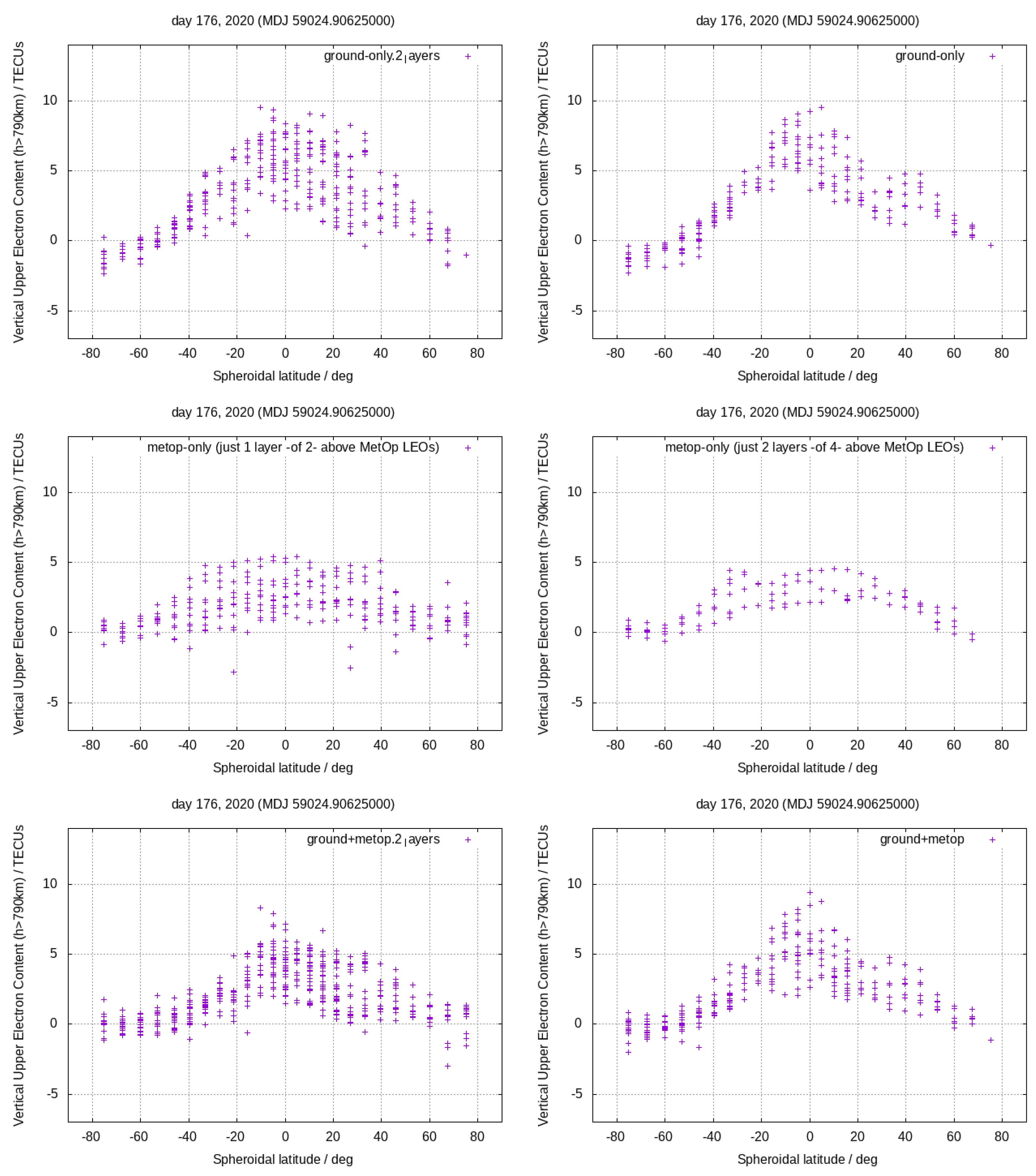
Abstract
1. Introduction
2. TOMION in a Nutshell
3. Methodology for DCB Retrieval
4. Data and Results
4.1. Ionospheric Tomography
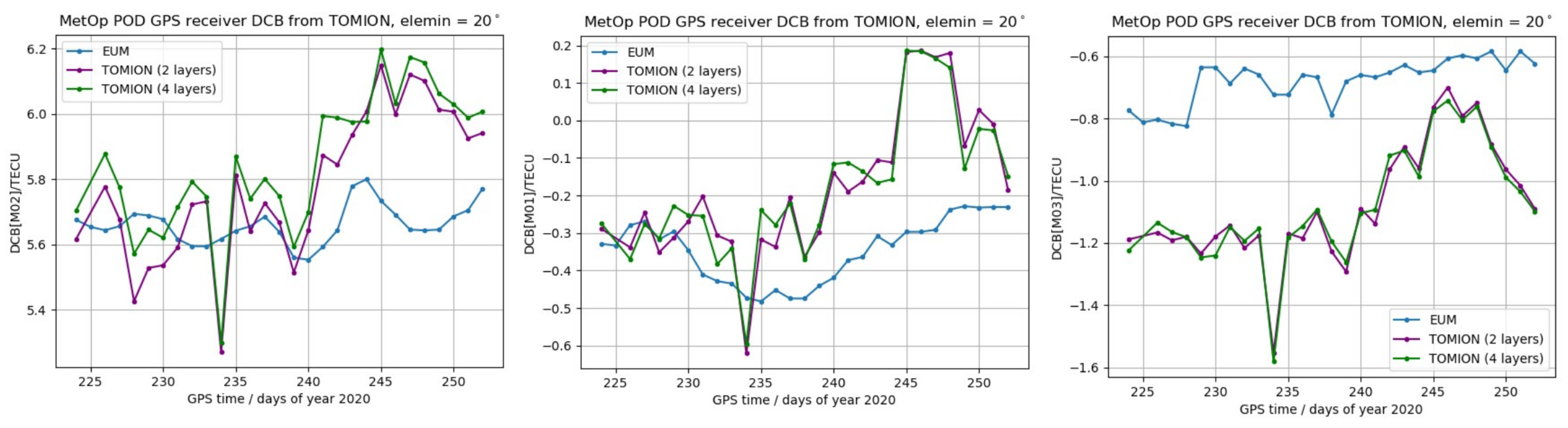
4.2. DCBs of MetOp POD GPS Receivers
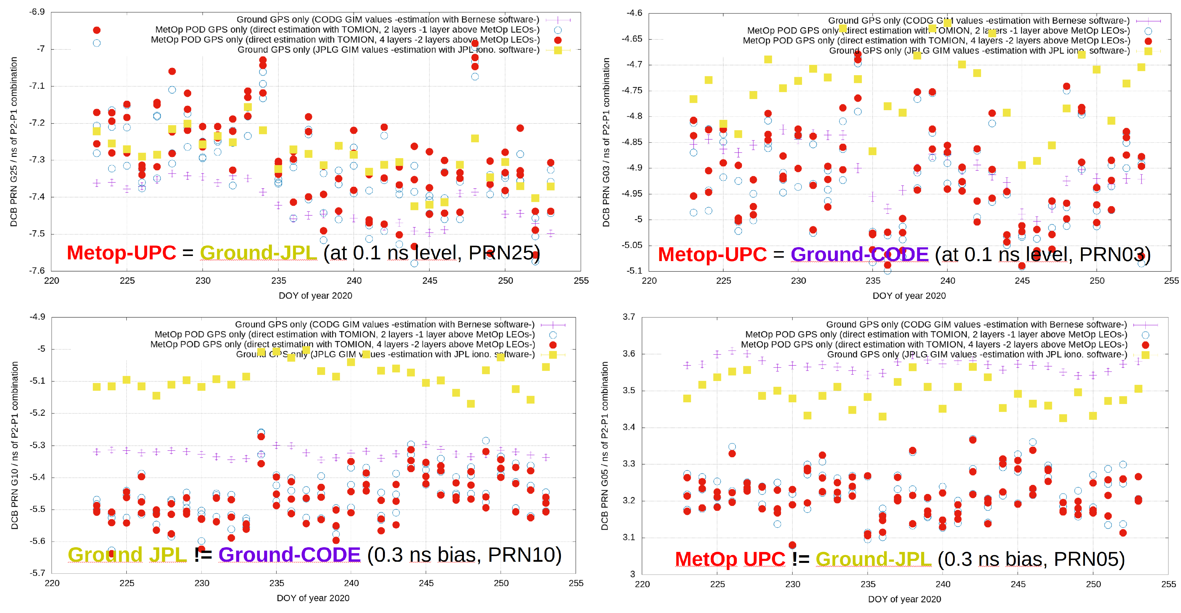
4.3. External Assessment via Transmitter DCBs
5. Discussion
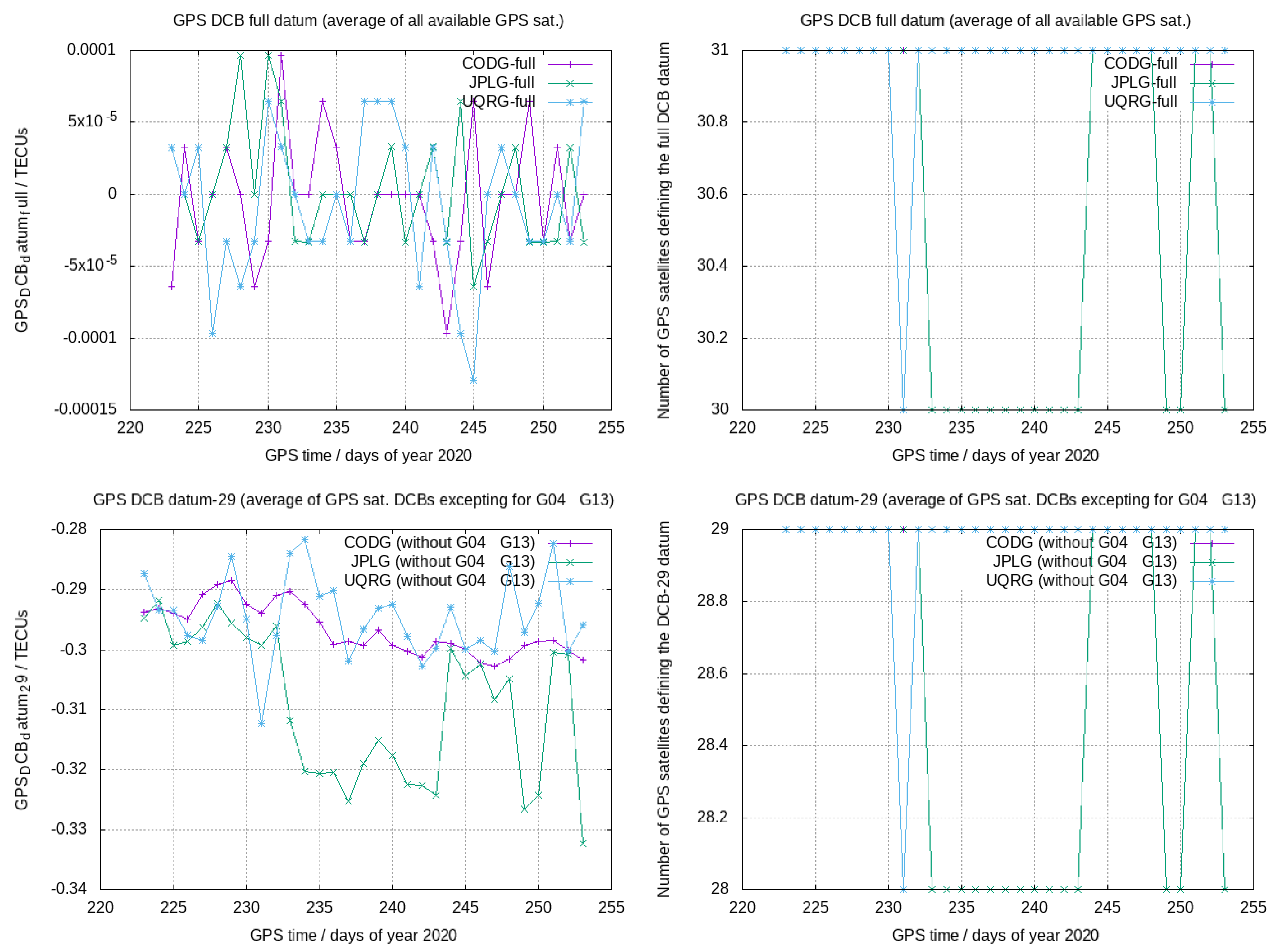
5.1. Influence of Changes in the DCB Data
5.2. Influence of the GPS Receiving Antenna Phase Center Variation
5.3. Potential Influence of the Difference between the LEO Orbits
6. Conclusions
Author Contributions
Funding
Data Availability Statement
Acknowledgments
Conflicts of Interest
Appendix A
References
- Hegarty, C.J.; Powers, E.D.; Fonville, B. Accounting for timing biases between GPS, modernized GPS and Galileo signals. In Proceedings of the 18th International Technical Meeting of the Satellite Division of The Institute of Navigation (ION GNSS 2005), Long Beach, CA, USA, 13–16 September 2005; pp. 2401–2407. [Google Scholar]
- Hauschild, A.; Montenbruck, O. A study on the dependency of GNSS pseudorange biases on correlator spacing. GPS Solut. 2016, 20, 159–171. [Google Scholar] [CrossRef]
- Xiang, Y.; Xu, Z.; Gao, Y.; Yu, W. Understanding long-term variations in GPS differential code biases. GPS Solut. 2020, 24, 1–11. [Google Scholar] [CrossRef]
- Prol, F.d.S.; Camargo, P.d.O.; Monico, J.F.G.; Muella, M.T.d.A.H. Assessment of a TEC calibration procedure by single-frequency PPP. GPS Solut. 2018, 22, 1–11. [Google Scholar] [CrossRef]
- Arikan, F.; Nayir, H.; Sezen, U.; Arikan, O. Estimation of single station interfrequency receiver bias using GPS-TEC. Radio Sci. 2008, 43, 1–13. [Google Scholar] [CrossRef]
- Mannucci, A.; Wilson, B.; Yuan, D.; Ho, C.; Lindqwister, U.; Runge, T. A Global mapping technique for GPS-derived ionospheric total electron content measurements. Radio Sci. 1998, 33, 565–582. [Google Scholar] [CrossRef]
- Sardon, E.; Rius, A.; Zarraoa, N. Estimation of the transmitter and receiver differential biases and the ionospheric total electron content from Global Positioning System observations. Radio Sci. 1994, 29, 577–586. [Google Scholar] [CrossRef]
- Sardón, E.; Zarraoa, N. Estimation of total electron content using GPS data: How stable are the differential satellite and receiver instrumental biases? Radio Sci. 1997, 32, 1899–1910. [Google Scholar] [CrossRef]
- Zhang, D.; Shi, H.; Jin, Y.; Zhang, W.; Hao, Y.; Xiao, Z. The variation of the estimated GPS instrumental bias and its possible connection with ionospheric variability. Sci. China Technol. Sci. 2014, 57, 67–79. [Google Scholar] [CrossRef]
- Zhong, J.; Lei, J.; Dou, X.; Yue, X. Is the long-term variation of the estimated GPS differential code biases associated with ionospheric variability? GPS Solut. 2016, 20, 313–319. [Google Scholar] [CrossRef]
- Zha, J.; Zhang, B.; Yuan, Y.; Li, M. Use of modified carrier-to-code leveling to analyze temperature dependence of multi-GNSS receiver DCB and to retrieve ionospheric TEC. GPS Solut. 2019, 23, 1–12. [Google Scholar] [CrossRef]
- Mi, X.; Zhang, B.; Odolinski, R.; Yuan, Y. On the temperature sensitivity of multi-GNSS intra-and inter-system biases and the impact on RTK positioning. GPS Solut. 2020, 24, 1–14. [Google Scholar] [CrossRef]
- Yue, X.; Schreiner, W.S.; Hunt, D.C.; Rocken, C.; Kuo, Y.H. Quantitative evaluation of the Low Earth Orbit satellite based slant total electron content determination. Space Weather 2011, 9. [Google Scholar] [CrossRef]
- Zhang, X.; Tang, L. Daily global plasmaspheric maps derived from cosmic GPS observations. IEEE Trans. Geosci. Remote Sens. 2014, 52, 6040–6046. [Google Scholar] [CrossRef]
- Lin, J.; Yue, X.; Zhao, S. Estimation and analysis of GPS satellite DCB based on LEO observations. GPS Solut. 2016, 20, 251–258. [Google Scholar] [CrossRef]
- Li, X.; Ma, T.; Xie, W.; Zhang, K.; Huang, J.; Ren, X. FY-3D and FY-3C onboard observations for differential code biases estimation. GPS Solut. 2019, 23, 1–14. [Google Scholar] [CrossRef]
- Zhong, J.; Lei, J.; Dou, X.; Yue, X. Assessment of vertical TEC mapping functions for space-based GNSS observations. GPS Solut. 2016, 20, 353–362. [Google Scholar] [CrossRef]
- Wautelet, G.; Loyer, S.; Mercier, F.; Perosanz, F. Computation of GPS P1–P2 differential code biases with Jason-2. GPS Solut. 2017, 21, 1619–1631. [Google Scholar] [CrossRef]
- Li, W.; Li, M.; Shi, C.; Fang, R.; Zhao, Q.; Meng, X.; Yang, G.; Bai, W. GPS and BeiDou differential code bias estimation using Fengyun-3C satellite onboard GNSS observations. Remote Sens. 2017, 9, 1239. [Google Scholar] [CrossRef]
- Yuan, L.; Jin, S.; Hoque, M. Estimation of LEO-GPS receiver differential code bias based on inequality constrained least square and multi-layer mapping function. GPS Solut. 2020, 24, 1–12. [Google Scholar] [CrossRef]
- Yuan, L.; Hoque, M.; Jin, S. A new method to estimate GPS satellite and receiver differential code biases using a network of LEO satellites. GPS Solut. 2021, 25, 1–12. [Google Scholar] [CrossRef]
- Heise, S.; Jakowski, N.; Wehrenpfennig, A.; Reigber, C.; Lühr, H. Sounding of the topside ionosphere/plasmasphere based on GPS measurements from CHAMP: Initial results. Geophys. Res. Lett. 2002, 29, 44-1–44-4. [Google Scholar] [CrossRef]
- Spencer, P.S.; Mitchell, C.N. Imaging of 3-D plasmaspheric electron density using GPS to LEO satellite differential phase observations. Radio Sci. 2011, 46, 1–6. [Google Scholar] [CrossRef]
- Wu, M.; Guo, P.; Xu, T.; Fu, N.; Xu, X.; Jin, H.; Hu, X. Data assimilation of plasmasphere and upper ionosphere using COSMIC/GPS slant TEC measurements. Radio Sci. 2015, 50, 1131–1140. [Google Scholar] [CrossRef]
- Kim, E.; Kim, Y.; Jee, G.; Ssessanga, N. Reconstruction of plasmaspheric density distributions by applying a tomography technique to jason-1 plasmaspheric TEC measurements. Radio Sci. 2018, 53, 866–873. [Google Scholar] [CrossRef]
- Prol, F.S.; Hoque, M.M. A Tomographic Method for the Reconstruction of the Plasmasphere Based on COSMIC/FORMOSAT-3 Data. IEEE J. Sel. Top. Appl. Earth Obs. Remote Sens. 2022, 15, 2197–2208. [Google Scholar] [CrossRef]
- Fu, N.; Guo, P.; Wu, M.; Huang, Y.; Hu, X.; Hong, Z. The two-parts step-by-step ionospheric assimilation based on ground-based/spaceborne observations and its verification. Remote Sens. 2019, 11, 1172. [Google Scholar] [CrossRef]
- Hernández-Pajares, M.; Juan, J.; Sanz, J. Neural network modeling of the ionospheric electron content at global scale using GPS data. Radio Sci. 1997, 32, 1081–1089. [Google Scholar] [CrossRef]
- Hernández-Pajares, M.; Juan, J.; Sanz, J. New approaches in global ionospheric determination using ground GPS data. J. Atmos. Sol.-Terr. Phys. 1999, 61, 1237–1247. [Google Scholar] [CrossRef]
- Orús, R.; Hernández-Pajares, M.; Juan, J.; Sanz, J. Improvement of global ionospheric VTEC maps by using kriging interpolation technique. J. Atmos. Sol.-Terr. Phys. 2005, 67, 1598–1609. [Google Scholar] [CrossRef]
- Roma Dollase, D. Global Ionospheric Maps: Estimation and Assessment in Post-Processing and Real-Time. Ph.D. Thesis, Universitat Politècnica de Catalunya, Barcelona, Spain, 2019. [Google Scholar]
- Hernández-Pajares, M.; Juan, J.M.; Sanz, J.; Aragón-Àngel, À.; García-Rigo, A.; Salazar, D.; Escudero, M. The ionosphere: Effects, GPS modeling and the benefits for space geodetic techniques. J. Geod. 2011, 85, 887–907. [Google Scholar] [CrossRef]
- Hernández-Pajares, M.; Juan, J.; Sanz, J.; Orus, R.; García-Rigo, A.; Feltens, J.; Komjathy, A.; Schaer, S.; Krankowski, A. The IGS VTEC maps: A reliable source of ionospheric information since 1998. J. Geod. 2009, 83, 263–275. [Google Scholar] [CrossRef]
- Hernández-Pajares, M.; Roma-Dollase, D.; Krankowski, A.; García-Rigo, A.; Orús-Pérez, R. Methodology and consistency of slant and vertical assessments for ionospheric electron content models. J. Geod. 2017, 91, 1405–1414. [Google Scholar] [CrossRef]
- Roma-Dollase, D.; Hernández-Pajares, M.; Krankowski, A.; Kotulak, K.; Ghoddousi-Fard, R.; Yuan, Y.; Li, Z.; Zhang, H.; Shi, C.; Wang, C.; et al. Consistency of seven different GNSS global ionospheric mapping techniques during one solar cycle. J. Geod. 2018, 92, 691–706. [Google Scholar] [CrossRef]
- Hernández-Pajares, M.; Lyu, H.; Aragón-Àngel, À.; Monte-Moreno, E.; Liu, J.; An, J.; Jiang, H. Polar Electron Content From GPS Data-Based Global Ionospheric Maps: Assessment, Case Studies and Climatology. J. Geophys. Res. Space Phys. 2020, 125, e2019JA027677. [Google Scholar] [CrossRef]
- Liu, Q.; Hernández-Pajares, M.; Lyu, H.; Nishioka, M.; Yang, H.; Monte-Moreno, E.; Gulyaeva, T.; Béniguel, Y.; Wilken, V.; Olivares-Pulido, G.; et al. Ionospheric Storm Scale Index Based on High Time Resolution UPC-IonSAT Global Ionospheric Maps (IsUG). Space Weather 2021, 19, e2021SW002853. [Google Scholar] [CrossRef]
- Hernández-Pajares, M.; Lyu, H.; Garcia-Fernandez, M.; Orus-Perez, R. A new way of improving global ionospheric maps by ionospheric tomography: Consistent combination of multi-GNSS and multi-space geodetic dual-frequency measurements gathered from vessel-, LEO-and ground-based receivers. J. Geod. 2020, 94, 1–16. [Google Scholar] [CrossRef]
- Kotov, D.; Richards, P.G.; Truhlík, V.; Bogomaz, O.; Shulha, M.; Maruyama, N.; Hairston, M.; Miyoshi, Y.; Kasahara, Y.; Kumamoto, A.; et al. Coincident observations by the Kharkiv IS radar and ionosonde, DMSP and Arase (ERG) satellites and FLIP model simulations: Implications for the NRLMSISE-00 hydrogen density, plasmasphere and ionosphere. Geophys. Res. Lett. 2018, 45, 8062–8071. [Google Scholar] [CrossRef]
- Kotov, D.; Richards, P.G.; Truhlík, V.; Maruyama, N.; Fedrizzi, M.; Shulha, M.; Bogomaz, O.; Lichtenberger, J.; Hernández-Pajares, M.; Chernogor, L.; et al. Weak magnetic storms can modulate ionosphere-plasmasphere interaction significantly: Mechanisms and manifestations at mid-latitudes. J. Geophys. Res. Space Phys. 2019, 124, 9665–9675. [Google Scholar] [CrossRef]
- Olivares-Pulido, G.; Hernández-Pajares, M.; Lyu, H.; Gu, S.; García-Rigo, A.; Graffigna, V.; Tomaszewski, D.; Wielgosz, P.; Rapiński, J.; Krypia-Gregorczyk, A.; et al. Ionospheric tomographic common clock model of undifferenced uncombined GNSS measurements. J. Geod. 2021, 95, 1–13. [Google Scholar] [CrossRef]
- Lyu, H.; Hernández-Pajares, M.; Nohutcu, M.; García-Rigo, A.; Zhang, H.; Liu, J. The Barcelona ionospheric mapping function (BIMF) and its application to northern mid-latitudes. GPS Solut. 2018, 22, 1–13. [Google Scholar] [CrossRef]
- Blewitt, G. An automatic editing algorithm for GPS data. Geophys. Res. Lett. 1990, 17, 199–202. [Google Scholar] [CrossRef]
- Jiahao, Z.; Lei, J.; Yue, X.; Dou, X. Determination of differential code bias of GNSS receiver onboard low Earth orbit satellite. IEEE Trans. Geosci. Remote Sens. 2016, 54, 4896–4905. [Google Scholar]
- Montenbruck, O.; Andres, Y.; Bock, H.; van Helleputte, T.; van den Ijssel, J.; Loiselet, M.; Marquardt, C.; Silvestrin, P.; Visser, P.; Yoon, Y. Tracking and orbit determination performance of the GRAS instrument on MetOp-A. GPS Solut. 2008, 12, 289–299. [Google Scholar] [CrossRef]


Disclaimer/Publisher’s Note: The statements, opinions and data contained in all publications are solely those of the individual author(s) and contributor(s) and not of MDPI and/or the editor(s). MDPI and/or the editor(s) disclaim responsibility for any injury to people or property resulting from any ideas, methods, instructions or products referred to in the content. |
© 2023 by the authors. Licensee MDPI, Basel, Switzerland. This article is an open access article distributed under the terms and conditions of the Creative Commons Attribution (CC BY) license (https://creativecommons.org/licenses/by/4.0/).
Share and Cite
Hernández-Pajares, M.; Olivares-Pulido, G.; Hoque, M.M.; Prol, F.S.; Yuan, L.; Notarpietro, R.; Graffigna, V. Topside Ionospheric Tomography Exclusively Based on LEO POD GPS Carrier Phases: Application to Autonomous LEO DCB Estimation. Remote Sens. 2023, 15, 390. https://doi.org/10.3390/rs15020390
Hernández-Pajares M, Olivares-Pulido G, Hoque MM, Prol FS, Yuan L, Notarpietro R, Graffigna V. Topside Ionospheric Tomography Exclusively Based on LEO POD GPS Carrier Phases: Application to Autonomous LEO DCB Estimation. Remote Sensing. 2023; 15(2):390. https://doi.org/10.3390/rs15020390
Chicago/Turabian StyleHernández-Pajares, Manuel, Germán Olivares-Pulido, M. Mainul Hoque, Fabricio S. Prol, Liangliang Yuan, Riccardo Notarpietro, and Victoria Graffigna. 2023. "Topside Ionospheric Tomography Exclusively Based on LEO POD GPS Carrier Phases: Application to Autonomous LEO DCB Estimation" Remote Sensing 15, no. 2: 390. https://doi.org/10.3390/rs15020390
APA StyleHernández-Pajares, M., Olivares-Pulido, G., Hoque, M. M., Prol, F. S., Yuan, L., Notarpietro, R., & Graffigna, V. (2023). Topside Ionospheric Tomography Exclusively Based on LEO POD GPS Carrier Phases: Application to Autonomous LEO DCB Estimation. Remote Sensing, 15(2), 390. https://doi.org/10.3390/rs15020390