Abstract
Advanced Earth observation technologies provide a tool for the study of ocean dynamics either in basins or in oceans. In a comparison of when and where, how ocean dynamics evolves in space and time is still a challenge. In view of an evolutionary scale, this paper proposes a novel approach to explore the evolutionary structures of ocean dynamics with time series of a raster dataset. This method, called PoEXES, includes three key steps. Firstly, a cluster-based algorithm is enhanced by process semantics to obtain marine snapshot objects. Secondly, the discriminant rule is formulated on the basis of successive marine snapshot objects’ spatiotemporal topologies to identify marine sequence objects and marine linked objects. Thirdly, a sequence-linked object-based algorithm (SLOA) is used for marine sequence objects and linked objects to obtain their evolutionary structures and to achieve four evolutionary relationships, i.e., development, merging, splitting, and a splitting–merging relationship. Using the evolutionary relationships and their occurring orders in a lifespan of ocean dynamics, this paper reformulates five types of evolutionary structures, which consist of origination nodes, linked nodes, sequence nodes and dissipation nodes. The evolutionary-scale-based dynamic structure ensures the optimum evolutionary relationships of ocean dynamics as much as possible, which provides a new way to design a spatiotemporal analysis model for dealing with geographical dynamics. To demonstrate the effectiveness and the advantages of PoEXES, a real 40-year dataset of satellite-derived sea surface temperatures is used to explore the evolutionary structure in global oceans; the new findings may help to better understand global climate change.
1. Introduction
Ocean dynamics provide information on when and where marine environments change as well as how they evolve in space and time [1,2]. In a comparison focusing on changes in terrestrial dynamics over time [3,4,5], the ocean dynamics focuses on the evolution in space and time [6]. This spatiotemporal evolution generally has a lifespan from origination, through development, merging, splitting, to finally dissipation [7]. It plays a significant role in regional and global climate change [2,8]; e.g., a merging or splitting of the sea surface temperature anomaly (SSTA) in the eastern-central Pacific Ocean will strengthen or weaken El Niño–Southern Oscillation (ENSO) intensity [9], a migration in space of SSTA helps to better identify the type of ENSO [10], a merging of mesoscale ocean eddies will generate a new one [11], and a splitting of an eddy will affect the eddy decay [12]. Additionally, advanced Earth-observing technologies make it possible to acquire lengthy time series of multiple remote sensing images from optical sensors, altimeters, scatterometers, and synthetic aperture radar imaging [13,14,15,16], which provide a foundation for the study of ocean dynamics in basins or global oceans [1,17,18].
The geographic world is dynamic [19,20]; it is categorized into instantaneous change and continuous change [21]. Instantaneous change occurs and then dissipates, e.g., land use and cover change, building of a new road, or a traffic accident. For the instantaneous geographic dynamics, object-/discrete event-based spatiotemporal models have been proposed to view spatial change as an occurrent object, with dynamic information incorporated into the time series of these occurrent objects [22,23]. On the basis of the above idea, object-oriented image analysis technologies were designed to identify geographic objects and analyze their dynamic changes [24,25,26], e.g., land use and cover change [4,5,24], or an urban heat island [3]. As dominated by human activities, these dynamics are discrete; thus, the aforementioned models are capable of dealing with the changes, not a real evolution in time.
Continuous change involves a certain time duration, e.g., an evolution of a typhoon or a rainstorm [27,28,29], a spread of a wildfire or a propagation of a disease [30], or an evolution of a marine abnormal variation [18,31]. To address such evolution over time, the process-/continuous-event-oriented model for analyzing geographical dynamics has received increased attention in recent years [7,9,32,33,34]. Yuan (2001) [30] designed a hierarchical framework of zone–sequence–process–event to address and analyze the dynamic characteristics of rainstorms in space and time. Restima and Albrecht (2005) [35] proposed a node–edge–node (NEN) model to represent and simulate geographical processes. Yi et al. (2014) [1] used a hierarchy of a static structure–process scenario to represent, track, query, and evaluate the oceanic eddies in the South China Sea. He et al. (2022) [36] designed the process–event-centered dynamic data model on the basis of the geographical scene framework to deal with geographic objects and their relationships with processes, events, and states. These models concern consistency over space and time as well as thematic elements among evolutionary entities and take the lifespan as a whole to represent and analyze geographic dynamics [23,31,37].
With an increase in computation abilities, many tracking approaches have been developed to obtain geographic dynamics. A spatiotemporal overlapping threshold-based method has been widely used for tracking rainstorms [38], flood events [39], dust storms [40], and changing clusters of remote sensing images [5,14]. With limited consideration of the moving characteristics of geographical dynamics, this algorithm has difficulty in effectively tracking fast-moving dynamics [29]. To address this deficiency, a number of modifications based on moving characteristics have been proposed for tracking rainstorms [27,28], oceanic eddies [41], marine heatwaves [42], marine abnormal variations [18,31], etc. For addressing the evolution of geographic dynamics, evolutionary relationships, i.e., the development, merging, splitting, splitting–merging, origination, dissipation, etc., have been proposed, designed, and obtained [9,40,43,44]. In addition, a graph-based model was developed to represent and store geographical objects, events, or processes and their evolutionary relationships, in which a node represents an object, an event, or a process, and an edge linking two nodes represents their relationship [3,9,27,28]. Through integrating the geographic objects’ characteristics at specific time snapshots and their moving characteristics among successive time snapshots, these event-oriented methods clearly address the evolution of the geographical dynamics.
These models and methods play a foundational role in addressing how ocean dynamics evolve in space and time. However, faced with ocean dynamics at previous–current–next snapshots, due to the lack of a full consideration of evolutionary characteristics, most of the existing methods are limited in their ability to explore evolutionary relationships [6]. The reason lies in that when the scale of data observation, i.e., a revisited cycle of satellite remote sensing or the temporal resolution of the dataset, is smaller than the scale of oceanic evolution, there may exist too many evolutionary relationships. Thus, when the evolutionary scale is smaller than the data observation scale, some key evolutionary relationships will be lost. In addition, most of the abovementioned methods consist of obtaining the evolutionary relationships of geographic dynamics [3,5,14,18,27,28,41]; exploring their evolutionary structures remains a challenge. Thus, further study is needed of to address the gap between the evolutionary relationship of geographic dynamics and the evolutionary structure.
To overcome the above deficiencies and to explore the evolutionary structures of ocean dynamics, this paper takes full consideration of the evolutionary characteristics of ocean dynamics to explore their evolutionary structures using time series of remote sensing images. We named our proposed method “Process-oriented exploring for the evolutionary structure of ocean dynamics”, or PoEXES. PoEXES allows progression from the exploration from evolutionary relationships to evolutionary structures, using time series of a remote sensing dataset, and contributes to marine data science research concerned with a spatiotemporal mining model for addressing ocean dynamics. In addition, the evolutionary structure of ocean dynamics helps to better understand the mechanism of marine environmental changes and provides a new reference for studying global climate change.
The remainder of this paper is organized as follows. Section 2 includes a workflow of PoEXES in view of an evolutionary scale and describes its key steps in detail. In Section 3, a time series dataset from global satellite-derived SST remote sensing images is used to evaluate PoEXES. Section 4 includes a discussion and conclusions.
2. Methods
2.1. Definitions
An ocean dynamic is an anomaly of the marine environment in space and time, and a marine anomaly has the evolutionary property of origination through development to dissipation. We define the evolutionary process from origination to dissipation as an evolutionary scale, and this paper takes the evolutionary scale to design PoEXES. Thus, some concepts about ocean dynamics and evolution need to be addressed from the perspective of algorithm design.
Marine anomaly refers to the abnormal increase or decrease in marine environmental parameters relative to the mean status of a long time series, which cover a specified spatial domain for a specified time range [17,31], e.g., monthly SSTA or seasonal sea surface salinity anomalies.
Marine evolutionary process refers to a marine phenomenon with a lifespan that has an evolution from origination through development to dissipation in space and time. This marine phenomenon may be a marine anomaly or an oceanic object, e.g., a sea level anomaly (SLA)-based eddy, whose spatial coverage with the value of SLA changes over time [1,45]. These changes of an eddy have an evolution property from origination through development to dissipation in space and time, and we define such an evolution as a process.
Marine evolutionary relationship refers to one of four relationships between successive time snapshots, i.e., a development, a merging, a splitting, and a splitting–merging [9]. Evolutionary relationships are shown in Figure 1 and Figure 2.
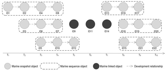
Figure 1.
The marine evolutionary process, including marine sequence objects, marine snapshot objects, marine linked objects, and the development relationships within sequence objects.
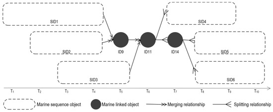
Figure 2.
The evolutionary structure of a process object, which consists of six sequence objects, three linked objects, and their merging and splitting relationships. The evolutionary structure omits the snapshot objects and their evolutionary relationships.
Marine snapshot object refers to an object of a marine anomaly at a specified time snapshot, generally a time of data observation, e.g., a SSTA object at a time in a satellite-passing territory.
Marine sequence object refers to an object generalized from time-order marine snapshot objects; it has similar evolutionary characteristics in space and is thematic within successive time snapshots. The spatial coverage of a marine sequence object is a union of all marine snapshot objects’ spatial coverages, and the time information of a marine sequence object ranges from the first to the last time snapshot of such objects.
Marine linked object refers to a special marine snapshot object, with which there exists at least one marine sequence object to be linked at successive previous or subsequent time snapshots.
Figure 1 and Figure 2 show the aforementioned definitions and their relationships. In Figure 1, we assume a marine process object that lasts for 10 snapshots and consists of 22 marine snapshot objects. Within the process object, 19 snapshot objects belong to 6 sequence objects, which are covered by dash rectangles, and 3 snapshot objects are linked objects, shown in back circles. The process object includes three kinds of evolutionary relationships; the development relationships are within sequence objects, shown in Figure 1, and the merging and splitting relationships are between sequence objects and linked objects, shown in Figure 2.
2.2. PoEXES Workflow
Marine snapshot objects belonging to the same sequence object have similar evolutionary characteristics in space and theme; that is, the spatial and thematic characteristics of snapshot objects can be simplified to the characteristics of a sequence object. Thus, PoEXES uses the sequence objects, linked objects, and their evolutionary relationships to represent oceanic evolutionary structure. Figure 2 gives an example of the evolutionary structure shown in Figure 1.
From time series of remote sensing images to the evolutionary structures of ocean dynamics, PoEXES needs to address three key steps. They are as follows: (1) the clustering-based algorithm is used to obtain the marine snapshot objects at each time snapshot one by one from the time series of remote sensing images; (2) an evolution-based tracking algorithm is designed to identify marine sequence objects and marine linked objects from marine snapshot objects; (3) the evolutionary relationships among marine sequence objects and marine linked objects are extracted to build the oceanic evolutionary structures. Figure 3 shows a workflow in which the three steps are the basis of the evolutionary characteristics of ocean dynamics, i.e., a lifespan from origination through development to dissipation.
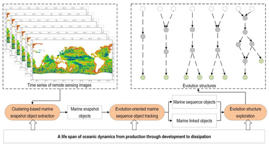
Figure 3.
Workflow of evolutionary structures of ocean dynamics from the time series of remote sensing images.
2.3. Clustering-Based Method of Extracting Marine Snapshot Objects
The core idea of dual-constraint spatiotemporal clustering approach (DcSTCA) takes the lifespan of a marine evolutionary process as an analyzing unit to deal with a time series of a remote sensing dataset, which includes the construction of a spatiotemporal neighborhood and the obtaining of spatiotemporal clustering cores. Considering the lifespan of a marine anomaly as a whole, DcSTCA performs well on spatiotemporal clustering patterns of SSTA in the Pacific Ocean [29]. Additionally, according to the definition of marine evolutionary process, a marine snapshot object belonging to the evolutionary process lasts for a specified time duration. Thus, this paper first adopts the DcSTCA to extract spatiotemporal clusters of marine anomalies. Then, the node searching method is used to vectorize a raster-formatted spatiotemporal cluster at each time snapshot to a polygon (object); that is, each cluster with grid cells at a time snapshot is transformed into one snapshot object. As only the snapshot objects in the previous–current–next time snapshots satisfying a certain degree of co-registration area (DCRA) can obtain the evolutionary relationships [3,16,27,29], this paper uses the DCRA between successive time snapshot objects to determine the marine snapshot objects.
The DCRA is calculated using Formula (1), where , and represent an object at a t − 1, t, and t + 1 snapshot, respectively; , and represent the spatial covered area of , and ; and and represent an co-registration area between and and between and , respectively.
When both and are greater than the specified threshold, the object is determined as a marine snapshot object; otherwise, the object is removed. Generally, the threshold is an empirical value. This paper uses 0.6 to determine marine snapshot objects.
Example 1:

Suppose the marine spatiotemporal cluster includes six objects of marine anomalies within three successive time snapshots: T − 1, T, and T + 1, as shown in Figure 4. As object 1, O1 at T snapshot overlaps with O1 at T − 1 snapshot and O1 at T + 1 snapshot, and the and satisfy the specified threshold; the O1 at T snapshot is regarded as a marine snapshot object. However, as O2 at T snapshot does not overlap with O2 at T − 1 snapshot and O2 at T + 1 snapshot, the O2 at T snapshot is not a marine snapshot object.

Figure 4.
An example of determining a marine snapshot object from a marine spatiotemporal cluster.
2.4. Evolution-Based Tracking Algorithm of Identifying Marine Sequence Objects and Marine Linked Objects
According to the definition of a marine sequence object, marine snapshot objects belonging to the sequence object have similar evolutionary characteristics in space and theme. Thus, there exist only development relationships among the successive marine snapshot objects; that is, there are no merging or splitting relationships. On this precondition, the identification of marine sequence objects and marine linked objects is as follows.
- Step 1: Denote marine snapshot objects at time snapshots T − 1, T, and T + 1 as , and , respectively, in which K, N, and M are the total number of marine snapshot objects at time snapshots T − 1, T, and T + 1, and , and are marine snapshot objects , and , respectively, in which k, i, and j relate to K, N and M, respectively.
- Step 2: Initialize marine snapshot objects at first time snapshot as candidates belonging to a marine sequence object, in which the time snapshot t equals zero. Then, set t to 1.
- Step 3: Calculate the spatial topologies between and and between and .
- Step 4: Formulate a discriminant rule on the basis of the spatial topology between and and the spatial topology between and , then determine as a marine linked object or as a marine sequence object.
Discriminant rule:
If there exists one and only one object spatially intersecting with and there exists one and only one spatially intersecting with , then is labeled as a candidate object belonging to the marine sequence object. Otherwise, is labeled as a marine linked object.
- Step 5: Where i = i + 1, repeat Step 3 and Step 4 until all the marine snapshot objects (i equals N) at time snapshot t, , are addressed.
- Step 6: Where t = t + 1, repeat Step 3 to Step 5 until the marine snapshot objects at all time snapshots (t equals T − 1) are addressed.
- Step 7: Those candidates belonging to marine sequence objects overlapped in space and time are linked together in an ascending time order to generate marine sequence objects, and those independent marine snapshot objects at successive times are identified as marine linked objects.
2.5. SLOA of Exploring Evolutionary Structures
Previous studies have produced process-oriented graphs depicting the ocean dynamics in detail [9]; however, there exist too many marine snapshot objects during the lifespan, which makes it difficult to directly represent its evolutionary structure. As marine snapshot objects belonging to the same sequence object have similar evolutionary characteristics in space and theme, the evolutionary structure based on the marine snapshot objects can be simplified and replaced by marine sequence objects. Figure 5 provides a workflow of the sequence-linked object-based algorithm (SLOA) of exploring evolutionary structures of ocean dynamics.
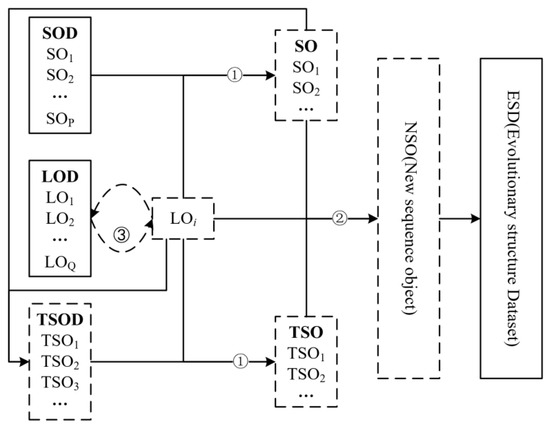
Figure 5.
Workflow of the sequence-linked object-based algorithm. SO, sequence object; TSO, temporary sequence object; LO, linked object; SOD, sequence object dataset; LOD, linked object dataset; TSOD, temporary sequence object dataset.
In Figure 5, there are three key issues: ① Given a specified marine linked object, obtain all its linked marine sequence objects from SOD and TSOD according to their spatiotemporal topologies, i.e., intersection in space and meet or met by in time; ② link all the marine linked objects and sequence objects to generate a new sequence object according to their meet or met-by temporal relationships; ③ create an iterative loop for marine linked objects until the new sequence object is updated. The details are as follows.
- Step 1: Denote marine sequence objects and their datasets as SOD-{SO1, SO2, ……, SOP}, denote marine linked objects and their datasets as LOD-{LO1, LO2, ……, LOQ}, and sort SOD and LOD in an ascending time order, in which P and Q are the total number of marine sequence objects and marine linked objects, respectively. Denote an evolutionary structure dataset, named ESD. Denote a temp sequence object dataset, named TSOD.
- Step 2: Set i to 1, and set TSOD as empty.
- Step 3: Obtain the ith marine linked object from LOD, i.e., LOi. Obtain all the marine sequence objects in SOD that satisfy the spatiotemporal topology with LOi, i.e., intersection in space and meet or met by in time, denoted as SO-{SO1, SO2, ……, SOk}. Obtain all items in TSOD that satisfy the intersection in space and meet or met by in time with LOi, denoted as TSO-{TSO1, TSO2, ……, TSOl}. Append {SO1, SO2, ……, SOk} to the TSOD.
- Step 4: Link the LOi with SO and TSO to generate a new sequence, named NSO, according to their temporal topologies. If meet applies, the relationship is from SOk or TSOl to LOi; if met by applies, the relationship is from TSOl to LOi or SOk.
- Step 5: Append LOi to the TSOD, i = i + 1, and repeat Step 3 and Step 4 until NSO is updated.
- Step 6: Append NSO to ESD, remove all the sequence objects in TSOD from SOD, remove all the linked objects in TSOD from LOD, and update SOD and LOD.
- Step 7: Repeat Step 2 to Step 6 until all the marine linked objects are addressed.
Here, Step 2 to Step 5 create a loop to obtain an evolutionary structure of one process object, and Step 2 to Step 7 finish all process objects’ structure. In the final ESD, each item represents an evolutionary structure of ocean dynamics. As is known, where and when the ocean dynamic generates and disappears play significant roles in regional and global climate changes, as do where and when the ocean dynamic merges and splits [1,9,27,46]. Thus, PoEXES expands the evolutionary structure of ocean dynamics by appending the marine snapshot objects when and where the evolution generates and dissipates.
2.6. Identification of Evolutionary Structure Types
According to the evolutionary relationships and their occurring order, this paper defines five types of evolutionary structure. Using a node–edge graph model, an in-degree and an out-degree of one node are calculated. The in-degree of a node is the number of edges directed into that node, and the out-degree is the number of edges directed out of that node. According to its in-degree and out-degree, the linked node is classified into three sub-nodes, i.e., a merging node, a splitting node, and a merging–splitting node, shown in Table 1.

Table 1.
Relationship between type of linked node and its in-degree and out-degree.
On the basis of the node–edge graph model, five types of evolutionary structure are defined, as shown in Figure 6.
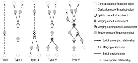
Figure 6.
Evolutionary structural types of ocean dynamics. Circles represent sequence objects, linked objects, or marine snapshot objects; arrows represent one of four evolutionary relationships.
- Evolutionary structural type I: There only exist development relationships in a lifespan of ocean dynamics. This structure has no linked node.
- Evolutionary structural type II: There exist development relationships and splitting relationships in a lifespan of ocean dynamics. This structure has at least one splitting node.
- Evolutionary structural type III: There exist development relationships and merging relationships in a lifespan of ocean dynamics. This structure has at least one merging node.
- Evolutionary structural type IV: There simultaneously exist development, merging, splitting, and splitting–merging relationships in a lifespan of ocean dynamics. This structure simultaneously has merging nodes and splitting nodes. Although sometimes the merging relationships alternate with the splitting ones, this structure has no form of ring.
- Evolutionary structural type V: There simultaneously exist development, merging, splitting, and splitting–merging relationships in a lifespan of ocean dynamics. Generally, there exists one or more merging relationships occurring after the splitting relationships, and this structure has the form of a ring, shown as type V in Figure 6.
3. Results and Discussions
3.1. Remote Sensing Datasets and Their Pretreatment
The SST remote sensing dataset used for the experiment is the NOAA Optimum Interpolation Sea Surface Temperature V2.0, provided by the NOAA/OAR/ESRL Physical Sciences Division, Boulder, Colorado, USA, and the details refer to literature [47]. The time period ranges from January 1982 to December 2021, with a spatial resolution of 1° and a temporal resolution of 1 month. The standard monthly average anomaly algorithm, denoted as the z-score [48], was used to remove seasonal variations of SST that were mainly dominated by solar radiance. Thus, the monthly global SSTA dataset for the period from January 1982 to December 2021 was generated to explore evolutionary structures of SSTA dynamics.
The multivariate ENSO index (MEI) provided by NOAA-ESRL Physical Sciences Division [49] is used for the definition of ENSO events in accordance with Ref. [8]. Eleven El Niño and nine La Niña events in the period from January 1982 to December 2021 were obtained and were used to analyze the relationships with evolutionary structures of SSTA dynamics.
3.2. Global Evolutionary Structures of SSTA Dynamics
According to whether the SSTA value was greater than zero or not, the process object was categorized into two classes: the warm process objects of SSTA and the cold ones. In total, we obtained 417 process objects from the aforementioned SSTA datasets, which include 230 warm process objects and 187 cold ones. Each process object corresponds to one evolutionary structural type, type I to type V. The details of process objects of SSTA and the five types of their evolutionary structures are shown in Table 2.

Table 2.
Types of evolutionary structure of SSTA dynamics in global oceans.
From Table 2, we know that 85% evolutionary structures of SSTA are type I, and they spread in global oceans, as shown in Figure 7. Their spatial information specifies where they originate, in which direction they move, and where they dissipate. Only the process objects with the evolutionary structural type I are shown in Figure 7; the other evolutionary structural types are omitted.
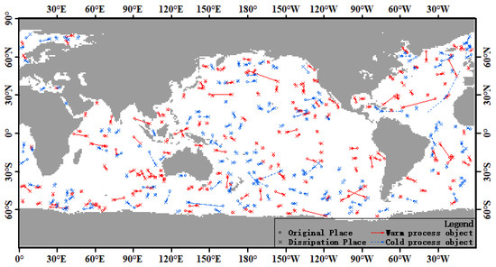
Figure 7.
Spatial distribution of evolutionary structure Type I of SSTA dynamics. Red arrows represent moving directions of warm process objects of SSTA; blue arrows represent moving directions of cold process objects of SSTA.
Table 2 also shows other types of evolutionary structures of SSTA. Although they are relatively small, most of them closely relate to signals of global climate change, e.g., ENSO, Indian Ocean Dipole (IOD), Pacific Decadal Oscillation (PDO). This paper takes ENSO and process objects of SSTA with type II as an example to analyze their interrelationships. The process object of SSTA related to ENSO events means that the time duration of an SSTA dynamic intersects with one of the ENSO events for at least three months.
Table 3 shows an example of corresponding relationships between evolutionary structure type II of SSTA dynamics and ENSO events. The interrelationship between type II and ENSO events shows that the evolutionary structure of an SSTA dynamic may be an indicator of an ENSO event and provides new insight for better understanding ENSO events.

Table 3.
Corresponding relationships between process objects of SSTA of type II and ENSO events. OID is the object identifier stored in database; duration of process object of SSTA is the number of months from origination to dissipation of SSTA.
3.3. Evolutionary Structure of a Specified SSTA Dynamic
A typical El Niño–Southern Oscillation (ENSO) event occurred during the period from January 1997 to December 1998 that affected a variety of marine environmental parameters [8]. As SSTA dynamics in the Pacific Ocean are more complex and sensitive to global climate change and regional sea–air interactions than in other regions, the SSTA dynamic occurring in the Central Eastern Pacific Ocean in a lifespan from February 1997 to December 1998 is considered as an example.
This SSTA dynamic consists of five evolutionary sequences. To clearly describe the evolution of this SSTA dynamic, Figure 8, Figure 9, Figure 10, Figure 11 and Figure 12 show the spatial distribution, the occurring period, and its evolution of sequence object 1 to sequence object 5; Figure 13 shows the spatial distribution of linked objects in June 1997, in which sequence object 1 and sequence object 2 merge into sequence object 3; and Figure 14 shows the spatial distribution of linked objects in May 1998, in which sequence object 3 splits sequence object 4 and sequence object 5.
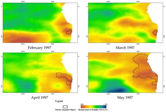
Figure 8.
Sequence object 1 originates and expands in the Eastern Pacific Ocean from February to May 1997. The background is the monthly SSTA.
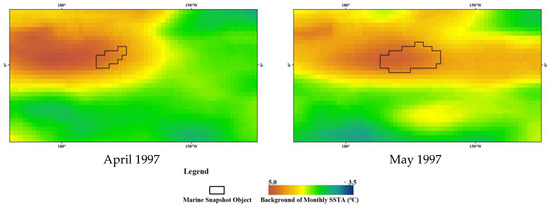
Figure 9.
Sequence object 2 originates and expands in the Equatorial Central Pacific Ocean from April to May 1997. The background is the monthly SSTA.
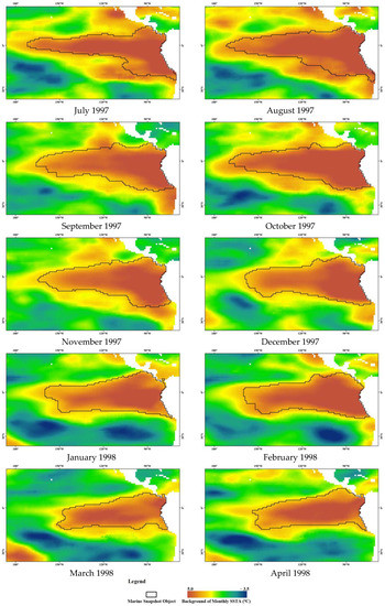
Figure 10.
Sequence object 3 develops in the Equatorial Eastern Pacific Ocean from July 1997 to April 1998. The background is the monthly SSTA.
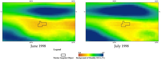
Figure 11.
Sequence object 4 continues to decrease in the Equatorial Central Pacific Ocean from June to July 1998. The background is the monthly SSTA.
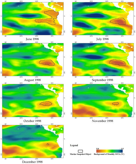
Figure 12.
Sequence object 5 continues to decrease in the Equatorial Eastern Pacific Ocean from June to December 1998. The background is the monthly SSTA.

Figure 13.
Linked object in June 1997, in which sequence object 1 and object 2 merge into sequence object 3 in the Equatorial Eastern Pacific Ocean. The background is the monthly SSTA.

Figure 14.
Linked object in May 1998, in which sequence object 3 splits sequence object 4 and object 5 in the Equatorial Eastern Pacific Ocean. The background is the monthly SSTA.
Figure 8, Figure 9, Figure 10, Figure 11 and Figure 12 show the details of space and time, in which this SSTA dynamic and its sequence objects occur, and Figure 13 and Figure 14 show the details of this SSTA dynamic and how it evolves in space and time. In February 1997, an SST abnormally increases and expands in the Eastern Pacific Ocean from March to May, which generates sequence object 1 (Figure 8). Meanwhile, in April 1997, an SST abnormally increases in the Equatorial Central Pacific Ocean and expands to May, which generates sequence object 2 (Figure 9). In June, sequence object 1 and sequence object 2 merge into and generate sequence object 3 in the Equatorial Eastern Pacific Ocean (Figure 13), where sequence object 3 continues to develop from July 1997 to April 1998 (Figure 10). In May 1998, sequence object 3 splits into sequence object 4 in the Central Eastern Pacific Ocean and sequence object 5 in the Eastern Pacific Ocean. From June 1998, sequence object 4 begins to shrink and disappears in the Equatorial Central Pacific Ocean in July 1998 (Figure 11), and sequence object 5 decreases and disappears in the Equatorial Eastern Pacific Ocean in December 1998 (Figure 12).
According to the proposed PoEXES, the evolutionary structure of the specified SSTA dynamic is obtained, and its sketch with detailed information is shown in Figure 15a. Figure 15b shows the SSTA dynamic and its corresponding sequence objects in space, and Figure 15c shows the evolutionary structure of the SSTA dynamic in space and time. In Figure 15c, the centroids are used to represent the spatial locations of sequence objects, original objects, and dissipation objects.
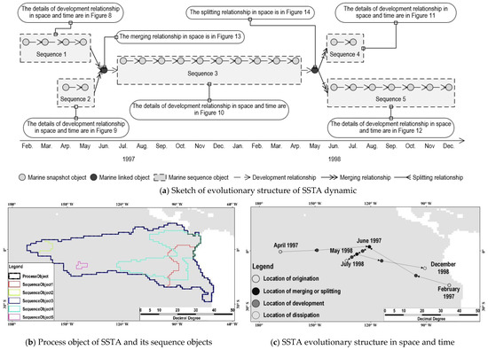
Figure 15.
Process object of SST and its evolutionary structure in space and time.
According to the definition of evolutionary structure type, this evolutionary structure is type IV. From such an evolutionary structure, we not only obtain when and where the SSTA originates, develops, and dissipates, but also when, where, and how the SSTA evolves (merges or splits). A comparison of Figure 15 and Figure 8, Figure 9, Figure 10, Figure 11, Figure 12, Figure 13 and Figure 14 shows that Figure 15 provides as much key spatiotemporal information of SSTA dynamics as Figure 8, Figure 9, Figure 10, Figure 11, Figure 12, Figure 13 and Figure 14. Moreover, the splitting or merging of this specified SSTA dynamic closely relates to the variation of ENSO intensity. Figure 16 shows the relationship between the merging and splitting of this SSTA dynamic with the strength and weakness of El Niño intensities, which occurred during the period of April 1997 to July 1998.
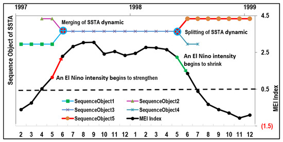
Figure 16.
Relationship between the evolutionary of SSTA dynamic and an El Niño event.
4. Conclusions
This paper follows our publication path of references [6,7,9,10,31,50] to track and connect ocean surface anomalies, which aims at describing ocean dynamics in a scale of evolutionary process. Compared to previous approaches, PoEXES designs the SLOA graph construction algorithm to identify evolutionary structures in a single- or multiple-linked graph.
The evolutionary structure of ocean dynamics identifies when, where, and how the marine abnormal variation evolves from origination through development to dissipation, which helps to better understand the changing mechanisms of marine environmental parameters. To explore such evolutionary structures from time series of raster-formatted SST datasets, we obtained five types of evolutionary structure of SSTA dynamics in global oceans using a 40-year SSTA dataset retrieved from remote sensing products, which proves the effectiveness and feasibility of PoEXES. The main conclusions drawn from this study and its contributions are summarized as follows.
(1) PoEXES was designed at a scale of dynamic evolution to explore the evolutionary structures of ocean dynamics, which ensures their evolutionary relationships are as optimal as possible. Generally, an evolutionary scale, which is from origination through development to death, is different from a scale of data observation. When taken directly from a time series of a dataset, the evolutionary relationships among time snapshots are too numerous to identify evolutionary structures when the evolutionary scale is greater than the data observation scale; when the evolutionary scale is smaller than the data observation scale, the key evolutionary relationships will be lost, and the evolutionary structure is incomplete.
(2) According to the merging, splitting, and splitting–merging relationships occurring or not, and the order of occurrence in a lifespan of ocean dynamics, this paper used the SLOA algorithm to identify five types of evolutionary structure. Type I is the simplest evolutionary structure, with only development relationships; type II to type IV consist of development and splitting relationships, development and merging relationships, and development, splitting, and merging relationships, respectively; and type V is the most complex, with a ring form, simultaneously consisting of merging, splitting, and splitting–merging relationships.
(3) We obtained 417 evolutionary structures of SSTA from remote sensing datasets in global oceans during the period of January 1982 to December 2021 and found that among them, 85% are type I, while the other types, especially type II to type IV, are more related to global climate changes, e.g., ENSO events.
The evolutionary structure consisting of origination nodes, linked nodes, and dissipation nodes not only identifies when and where marine environments change but also how they change, which helps to explore why they change. Five types of evolutionary structure not only refer to the theoretically possible structures derived from our designed SLOA, but also to those detected when applying the real dataset. Although only a real SST dataset is used as a case study to evaluate the PoEXES performance, PoEXES will achieve similar capabilities when dealing with sea surface salinity, sea level anomaly, etc. PoEXES takes an evolutionary scale to concentrate on a method of processing time series of remote sensing datasets, which contributes to time series of remote sensing data treatment and helps to find their dynamic patterns. In addition, PoEXES provides a new way to simultaneously analyze the spatial, temporal, and thematic characteristics of ocean dynamics, which contributes to GIScience research concerned with a spatiotemporal mining model for addressing geographical dynamics.
PoEXES includes a promising temporal scale for analyzing ocean dynamics; however, one limitation should be pointed out, which is that by taking the evolutionary sequence to simplify the oceanic dynamics, PoEXES will lose some spatial and temporal information when dealing with the successive multiple alternating merging and splitting oceanic dynamics. A large number of evolutionary structures of SSTA have been found in global oceans. Some of them are known, and some of them are less known, e.g., interrelationships with IOD and PDO; these relationships are in need of further research. Additionally, this study only adopts SSTA as one case to evaluate PoEXES; such highly dynamic processes (e.g., mesoscale eddy, oceanic front) should be further examined and tracked by the proposed PoEXES.
Author Contributions
Conceptualization, C.X. and F.S.; methodology, C.X. and C.N.; software, Y.X. and C.N.; data curation, C.N. and Y.X.; writing—original draft preparation, C.X. and Y.X.; writing—review and editing, C.X. and F.S.; supervision, F.S.; project administration, C.X.; funding acquisition, C.X. All authors have read and agreed to the published version of the manuscript.
Funding
This research was supported by the Strategic Priority Research Program of the Chinese Academy of Sciences (No. XDA19060103) and by the Innovative Research Program of the International Research Center of Big Data for Sustainable Development Goals (No. CBAS2022IRP05). The APC was funded by XDA19060103.
Data Availability Statement
Not applicable.
Acknowledgments
We thank the NASA/JPL/PO.DAAC for providing the research data.
Conflicts of Interest
The authors declare no conflict of interest.
References
- Yi, J.W.; Du, Y.Y.; Liang, F.Y.; Zhou, C.H.; Wu, D.; Mo, Y. A representation framework for studying spatiotemporal changes and interactions of dynamic geographic phenomena. Int. J. Geogr. Inf. Sci. 2014, 28, 1010–1027. [Google Scholar] [CrossRef]
- Yuan, M. Why are events important and how to compute them in geospatial research? J. Spat. Inf. Sci. 2020, 21, 47–61. [Google Scholar] [CrossRef]
- Zhu, R.; Guilbert, E.; Wong, M.D. Object-oriented tracking of the dynamic behavior of urban heat islands. Int. J. Geogr. Inf. Sci. 2017, 31, 405–424. [Google Scholar] [CrossRef]
- Atluri, G.; Karpatne, A.; Kumar, V. Spatio-Temporal Data Mining: A Survey of Problems and Methods. ACM Comput. Surv. 2018, 51, 1–41. [Google Scholar] [CrossRef]
- Khiali, L.; Ndiath, M.; Alleaume, S.; Lenco, D.; Ose, K.; Teisseire, M. Detection of spatio-temporal evolutions on multi-annual satellite image time series: A clustering-based approach. Int. J. Appl. Earth Obs. Geoinf. 2019, 74, 103–119. [Google Scholar] [CrossRef]
- Xue, C.J.; Su, F.Z.; He, Y.W. Process:A new view of geographical spatiotemporal dynamic analysis. Adv. Earth Sci. 2022, 37, 65–79. (In Chinese) [Google Scholar]
- Xue, C.J.; Dong, Q.; Xie, J. Marine spatio-temporal process semantics and its application-taking the El Nino Southern Oscilation process and Chinese rainfall anomaly as an example. Acta Oceanol. Sin. 2012, 31, 16–24. [Google Scholar] [CrossRef]
- McPhaden, M.J.; Stephen, E.; Zebia, K.; Michael, H. Glantz. ENSO as an integrating concept in earth science. Science 2006, 314, 1740–1745. [Google Scholar] [CrossRef] [PubMed]
- Xue, C.J.; Wu, C.; Liu, J.; Su, F. A novel process-oriented graph Storage for dynamic geographic phenomena. ISPRS Int. J. Geo-Inf. 2019, 8, 100. [Google Scholar] [CrossRef]
- Liu, J.Y.; Xue, C.J.; Dong, Q.; Wu, C.B.; Xu, Y.F. A Process-Oriented Spatiotemporal Clustering Method for Complex Trajectories of Dynamic Geographic Phenomena. IEEE Access 2019, 23, 155951–155964. [Google Scholar] [CrossRef]
- Fang, F.; Morrow, R. Evolution, movement and decay of warmcore Leeuwin Current eddies. Deep-Sea Res. Part II 2003, 50, 2245–2261. [Google Scholar] [CrossRef]
- Rodríguez, R.; Viudez, A.; Ruiz, S. Vortex Merger in Oceanic Tripoles. J. Phys. Oceanogr. 2011, 41, 1239–1251. [Google Scholar] [CrossRef]
- Yang, J.; Gong, P.; Fu, R.; Zhang, M.H.; Chen, J.M.; Liang, S.L.; Xu, B.; Shi, J.C.; Dickinson, R. The role of satellite remote sensing in climate change studies. Nat. Clim. Chang. 2013, 3, 875–883. [Google Scholar] [CrossRef]
- Guttler, F.; Lenco, D.; Nin, J.; Teisseire, M.; Poncelet, P. A graph-based approach to detect spatiotemporal dynamics in satellite image time series. ISPRS J. Photogramm. Remote Sens. 2017, 130, 92–107. [Google Scholar] [CrossRef]
- Chen, K.S. Principles of Synthetic Aperture Radar Imaging: A System Simulation Approach (Signal and Image Processing of Earth Observations); CRC Press, Inc.: Boca Raton, FL, USA, 2015. [Google Scholar]
- Jackson, C. Synthetic Aperture Radar Marine User’s Manual; United States Government Printing Office: Washington, DC, USA, 2004. [Google Scholar]
- Xue, C.J.; Song, W.J.; Qin, L.J.; Dong, Q.; Wen, X.Y. A spatiotemporal mining framework for abnormal association patterns in marine environments with a time series of remote sensing images. Int. J. Appl. Earth Obs. Geoinf. 2015, 38, 105–114. [Google Scholar] [CrossRef]
- Li, L.W.; Xu, Y.; Xue, C.J.; Fu, Y.; Zhang, Y. A Process-Oriented Approach to Identify Evolutions of sea surface salinity Temperature Anomalies with a Time-Series of a Raster Dataset. ISPRS Int. J. Geo-Inf. 2021, 10, 500. [Google Scholar] [CrossRef]
- Yuan, M.; Mark, D.M.; Egenhofer, M.J.; Peuquet, D.J. Extensions to Geographic Representation: A Research Agenda for Geographic Information Science; CRC Press: Boca Raton, FL, USA, 2004; pp. 129–156. [Google Scholar]
- Shaw, S.-L.; Ye, X. Capturing Spatiotemporal Dynamics in Computational Modeling. In The Geographic Information Science & Technology Body of Knowledge (1st Quarter 2019 Edition); Wilson, J.P., Ed.; University Consortium for Geographic Information Science: Washington, DC, USA, 2019. [Google Scholar] [CrossRef]
- Worboys, M.F. Event-oriented approaches to geographic phenomena. Int. J. Geogr. Inf. Sci. 2005, 19, 1–28. [Google Scholar] [CrossRef]
- Hornsby, K.; Egenhofer, M. Identity-based change: A foundation for spatio-temporal knowledge representation. Int. J. Geogr. Inf. Sci. 2000, 3, 207–224. [Google Scholar] [CrossRef]
- Nixon, V.; Hornsby, K.S. Using geolifespans to model dynamic geographic domains. Int. J. Geogr. Inf. Sci. 2010, 24, 1289–1308. [Google Scholar] [CrossRef]
- Wu, B.; Yu, B.; Shu, S.; Wu, Q.; Zhao, Y.; Wu, J. A spatiotemporal structural graph for detecting land cover changes. Int. J. Geogr. Inf. Sci. 2021, 35, 397–425. [Google Scholar] [CrossRef]
- Fichera, C.R.; Modica, G.; Pollino, M. Land Cover classification and change-detection analysis using multi-temporal remote sensed imagery and landscape metrics. Eur. J. Remote Sens. 2012, 45, 1–18. [Google Scholar] [CrossRef]
- Yan, J.; Wang, L.; Song, W.; Chen, Y. A time-series classification approach based on change detection for rapid land cover mapping. ISPRS J. Photogramm. Remote Sens. 2019, 158, 249–262. [Google Scholar] [CrossRef]
- Liu, W.B.; Li, X.G.; Rahn, D.A. Storm event representation and analysis based on a directed spatiotemporal graph model. Int. J. Geogr. Inf. Sci. 2016, 30, 1–22. [Google Scholar] [CrossRef]
- Muñoz, C.; Wang, L.P.; Willems, P. Enhanced object-based tracking algorithm for convective rainstorms and cells. Atmos. Res. 2018, 201, 144–158. [Google Scholar] [CrossRef]
- Xue, C.J.; Liu, J.Y.; Yang, G.H.; Wu, C.B. A process-oriented method for tracking rainstorms with a time-series of raster datasets. Appl. Sci. 2019, 9, 2468. [Google Scholar] [CrossRef]
- Yuan, M. Representing complex geographic phenomena in GIS. Cartogr. Geogr. Inf. Sci. 2001, 28, 83–96. [Google Scholar] [CrossRef]
- Liu, J.; Xue, C.; He, Y.; Dong, Q.; Kong, F.; Hong, Y. Dual-constraint Spatiotemporal Clustering Approach for Exploring Marine Anomaly Patterns using Remote Sensing Products. IEEE J. Sel. Top. Appl. Earth Obs. Remote Sens. 2018, 11, 3963–3976. [Google Scholar] [CrossRef]
- Long, J.A.; Nelson, T.A. A review of quantitative methods for movement data. Int. J. Geogr. Inf. Sci. 2013, 27, 292–318. [Google Scholar] [CrossRef]
- Kwan, M.P.; Neutens, T. Space-Time Research in GIScience. Int. J. Geogr. Inf. Sci. 2014, 25, 851–854. [Google Scholar] [CrossRef]
- Anthony, J.; Suzana, D. Towards a voxel-based geographic automata for the simulation of geospatial processes. Isprs. J. Photogramm. 2016, 117, 206–216. [Google Scholar]
- Reitsma, F.; Albrecht, J. Implementing a new data model for simulating processes. Int. J. Geogr. Inf. Sci. 2005, 10, 19,1073–1090. [Google Scholar] [CrossRef]
- He, Y.F.; Sheng, Y.H.; Hofer, B.; Huang, Y.; Qin, J.R. Processes and events in the centre: A dynamic data model for representing spatial change. Int. J. Digit. Earth 2022, 15, 276–295. [Google Scholar] [CrossRef]
- Campelo, C.E.C.; Bennett, B.; Dimitrova, V. Identifying Geographical Processes from Time-Stamped Data. In GeoSpatial Semantics, GeoS 2011; Lecture Notes in Computer Science; Claramunt, C., Levashkin, S., Bertolotto, M., Eds.; Springer: Berlin/Heidelberg, Germany, 2011; p. 6631. [Google Scholar]
- Dixon, M.; Wiener, G. TITAN: Thunderstorm identification, tracking, analysis, and nowcasting—A radar-based methodology. J. Atmos. Ocean. Technol. 1993, 10, 785–797. [Google Scholar] [CrossRef]
- Debusscher, B.; Coillie, F.M.B.V. Object-Based Flood Analysis Using a Graph-Based Representation. Remote Sens. 2019, 11, 1883. [Google Scholar] [CrossRef]
- Yu, M.; Yang, C.; Jin, B. A Framework for Natural Phenomena Movement Tracking–Using 4D Dust Simulation as an Example. Comput. Geosci. 2018, 121, 53–66. [Google Scholar] [CrossRef]
- Wang, H.; Du, Y.; Yi, J.; Sun, Y.; Liang, F. A new method for measuring topological structure similarity between complex trajectories. IEEE Trans. Knowl. Data Eng. 2019, 31, 1836–1848. [Google Scholar] [CrossRef]
- Lo, S.H.; Chen, C.T.; Russo, S.; Huang, W.R.; Shih, M.F. Tracking heatwave extremes from an event perspective. Weather Clim. Extrem. 2021, 34, 100371. [Google Scholar] [CrossRef]
- Mondo, G.D.; Rodríguez, M.A.; Claramunt, C.; Bravo, L.; Thibaud, R. Modelling consistency of spatio-temporal graphs. Data Knowl. Eng. 2013, 84, 59–80. [Google Scholar] [CrossRef]
- Mondo, G.D.; Stell, J.G.; Claramunt, C.; Thibaud, R. A graph model for spatio-temporal evolution. J. UCS 2010, 16, 1452–1477. [Google Scholar]
- Chen, G.X.; Hou, Y.J.; Chu, X.Q.; Qi, P. Vertical structure and evolution of the Luzon Warm Eddy. Chin. J. Oceanol. Limnol. 2010, 28, 955–961. [Google Scholar] [CrossRef]
- Yu, M.; Bambacus, M.; Cervone, G.; Clarke, K.; Duffy, D.; Huang, Q.; Li, J.; Li, W.; Li, Z.; Liu, Q.; et al. Spatiotemporal event detection: A review. Int. J. Digit. Earth 2020, 13, 1–27. [Google Scholar] [CrossRef]
- Reynolds, R.W.; Rayner, N.A.; Smith, T.M.; Stokes, D.C.; Wang, W. An Improved In Situ and Satellite SST Analysis for Climate. J. Clim. 2002, 15, 1609–1625. [Google Scholar] [CrossRef]
- Zhang, P.; Steinbach, M.; Kumar, V.; Shekhar, S.; Tan, P.-N.; Klooster, S.; Potter, C. Discovery of patterns of Earth Science Data Using Data Mining. In Next Generation of Data Mining Applications; Zurada, J., Kantardzic, M., Eds.; IEEE Press: Piscataway, NJ, USA, 2005; pp. 167–188. [Google Scholar]
- Wolter, K.; Timlin, M.S. El Nino/Southern Oscillation behavior since 1871 as diagnosed in an extended multivariate ENSO index (MEI.ext). Int. J. Climatol. 2011, 31, 1074–1087. [Google Scholar] [CrossRef]
- Xue, C.J.; Xu, Y.F.; He, Y.W. A global process-oriented sea surface temperature anomaly dataset retrieved from remote sensing products. Big Earth Data 2022, 6, 179–195. [Google Scholar] [CrossRef]
Disclaimer/Publisher’s Note: The statements, opinions and data contained in all publications are solely those of the individual author(s) and contributor(s) and not of MDPI and/or the editor(s). MDPI and/or the editor(s) disclaim responsibility for any injury to people or property resulting from any ideas, methods, instructions or products referred to in the content. |
© 2023 by the authors. Licensee MDPI, Basel, Switzerland. This article is an open access article distributed under the terms and conditions of the Creative Commons Attribution (CC BY) license (https://creativecommons.org/licenses/by/4.0/).