Abstract
Although many machine learning methods have been successfully applied for the object-based classification of high resolution (HR) remote sensing imagery, current methods are highly dependent on the spectral similarity between segmented objects and have disappointingly poor performance when dealing with different segmented objects that have similar spectra. To overcome this limitation, this study exploited a knowledge graph (KG) that preserved the spatial relationships between segmented objects and has a reasoning capability that can assist in improving the probability of correctly classifying different segmented objects with similar spectra. In addition, to assist the knowledge graph classifications, an image segmentation method generating segmented objects that closely resemble real ground objects in size was used, which improves the integrity of the object classification results. Therefore, a novel HR remote sensing image classification scheme is proposed that involves a knowledge graph and an optimal segmentation algorithm, which takes full advantage of object-based classification and knowledge inference. This method effectively addresses the problems of object classification integrity and misclassification of objects with the same spectrum. In the evaluation experiments, three QuickBird-2 images and over 15 different land cover classes were utilized. The results showed that the classification accuracy of the proposed method is high, with overall accuracies exceeding 0.85. These accuracies are higher than the K Nearest Neighbors (KNN), Support Vector Machine (SVM), Decision Tree (DT), and Random Forest (RF) methods. The evaluated results confirmed that the proposed method offers excellent performance in HR remote sensing image classification.
1. Introduction
In recent decades, with increasing advances in remote sensing technology and the growing demand for remote sensing applications, high resolution (HR) remote sensing (RS) imagery (approximately 1–3 m) has gradually emerged and seen wide adoption [1]. Pixel-based methods were first used for land cover analyses using HR remote sensing imagery. However, pixel-based methods easily fail to exploit the relationships within neighboring pixels, which leads to unsatisfactory classification results, such as the appearance of salt and pepper noise [2]. Geographic object-based image analysis (GEOBIA) can fully consider the spatial relationships between adjacent pixels and address numerous problems appearing in pixel-based analysis [3]. Therefore, since its introduction, GEOBIA has been gradually favored by researchers [4,5,6].
GEOBIA methods consider the image object as the basic analysis unit, rather than a single pixel [7]. The goal of GEOBIA is to address the complex spatial and hierarchical relationships between image pixels and reduce the classification error rate for HR remote sensing imagery [8]. Due to GEOBIA outputs, image classification has become a crucial element in the overall analytical process; the results of which impact the decisions of remote sensing analysts and determine how remote sensing data is ultimately used [9].
Numerous classifiers for HR remote sensing imagery have been applied in GEOBIA [10,11,12]. For example, the K Nearest Neighbors (KNN) method [13], Decision Tree (DT) method [14], Random Forest (RF) method [15], and Support Vector Machine (SVM) method [16] have already seen widespread adoption in classification tasks. These methods construct a multidimensional feature classifier by selecting a number of training samples to generate a multidimensional membership function, which is used to calculate the probability that each classification object belongs to each class before outputting the maximum classification probability as the result. These methods essentially use the statistical relation between the training sample and the object to be classified to perform the classification., i.e., the spectral response and shape similarities between the training sample and the object to be classified are the main dependencies for these methods. Some misclassifications frequently occur because the spatial and contextual relationships between neighboring objects are ignored. Therefore, how to completely utilize the various spatial and contextual relationships between neighboring image objects to assist in image classification is also a fundamental problem that it is crucial to solve.
Google introduced the knowledge graph in 2012 and it has since seen rapid use and adoption [17,18,19]. A knowledge graph is a multirelational graph composed of nodes and various types of directed edges that preserve numerous spatial and contextual relationships inherent in remote sensing imagery [20]. Previous classification methods, which ignore the relationships between image segmented objects in the process, are inconsistent with Tobler’s First Law of Geography, which considers the relationships between the neighbors instead of the objects themselves [21]. The large set of relationships within the knowledge graph endows the knowledge graph with the ability of knowledge reasoning. Therefore, a better classification result could be procured by employing a knowledge graph that fully incorporates the relationships between segmented objects and integrates these relationships into the object recognition process within GEOBIA. Current existing works consider knowledge graphs as a semantic representational database by constructing a natural language model to provide knowledge reasoning capability for remote sensing image interpretation. For example, Li et al. (2021) [18] constructed a new remote sensing knowledge graph from scratch to support the inference recognition of unseen remote sensing images. In [22], the authors demonstrated the promising capability of remote sensing semantic reasoning in the intelligent remote sensing image interpretation field by constructing a semantic knowledge graph. However, as a relational database, both the data query (query matching using similarity of attributes of image objects) and knowledge inference capabilities of the knowledge graph are advantages worth investigating in remote sensing image interpretation.
The purpose of this study is to make full use of the data query and knowledge inference capabilities of knowledge graphs to classify imagery and address some misclassification problems caused by ignoring the spatial and contextual relationships between image segmented objects. To achieve this goal, a novel knowledge graph-based classification method for HR remote sensing imagery is proposed. To consider the benefit of both data query and knowledge inference in the knowledge graph, after building the knowledge graph, we divide the knowledge graph-based object recognition approaches into two categories. One is to classify objects by using the similarity of attributes between segmented objects and objects in the knowledge graph directly to perform object query and matching. The other category is to determine the affiliation class of segmented objects based on the spatial and contextual relationships stored in the knowledge graph. Notably, the image segmentation method proposed by [23] is employed in our work, which produces two main types of segmented objects, one with a size close to the real ground objects (named a significant object) and another oversegmented object with a size much smaller than the real ground objects. Therefore, these two types of objects apply to each of the two object recognition approaches mentioned above. Accordingly, we complete the whole classification process in the following steps. First, we construct the knowledge graph by manually vectorizing image objects to extract object attributes and spatial relationships. In addition, to facilitate the query and matching of segmented objects, an unidentified object graph that has the same data storage structure as the knowledge graph has been established based on segmented objects. Second, we have managed to recognize significant objects using the established rules defining the similarity of objects found in the knowledge graph and the unidentified object graph. Then, to improve the completeness of the significant objects, a merging process is performed involving the significant object and surrounding unidentified objects. Third, we integrate the contextual relationships to recognize smaller objects with inconspicuous characteristics and iterate the above steps as needed. Finally, a robust classification result was derived by integrating the spatial relationships to adjust the misclassifications. The proposed method has made two main contributions. First, knowledge graphs, which were utilized to store various relationships between image objects, have been used to successfully classify HR remote sensing imagery. Second, unlike classifying oversegmented objects in terms of their characteristics, this study aims to leverage the data query and knowledge inference capabilities of knowledge graphs to recognize land covers, which provides a novel approach of remote sensing image classification. Experimental results show that a satisfactory classification result can be attained via the proposed method for various types of land cover.
2. Methodology
The objective of our work was to investigate a classification method for high-resolution (HR) remote sensing imagery using a remote sensing knowledge graph. Figure 1 illustrates the systematic process of the classification method. First, HR remote sensing imagery with typical feature objects was selected for data preprocessing and image vectorization to construct reference imagery, and then the typical feature objects in the reference imagery were extracted to construct a knowledge graph composed of the object tree. Second, the established knowledge graph was used to match and identify the classes of objects within the segmentation graph that are produced by the segmentation image derived from the image segmentation algorithm. Finally, the final classification results were output based on the probability that the matched and inferred objects are affiliated with a class.
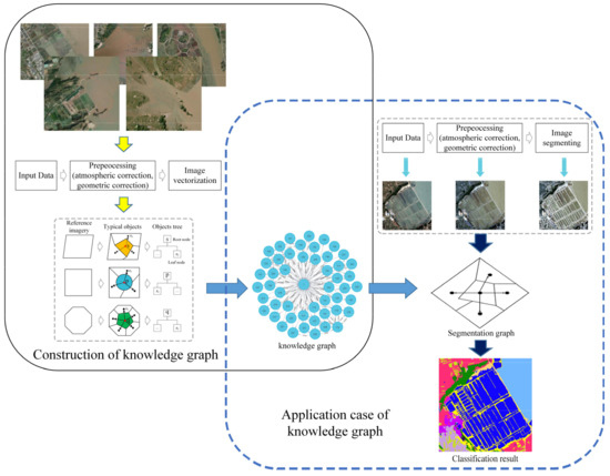
Figure 1.
Systematic process of the proposed method. s, p, and q represent the oversegmented objects, while symbolizes the neighbors of the oversegmented object.
Note that the proposed method combines the segmentation algorithm and knowledge graph to achieve classification; thus, the segmentation algorithm is crucial as well. This segmentation algorithm, proposed by [23], generates two main types of segmented objects: one with a size close to the real ground objects (named significant objects) and another oversegmented object with a size much smaller than the real ground objects. To achieve the desired classification effect in these two types of segmented objects, this study developed five steps. Figure 2 depicts the framework of the proposed method. First, knowledge graphs are constructed based on the reference imagery established from the original HR remote sensing imagery. In addition, to facilitate the matching of objects to be classified with objects in the knowledge graph, an unidentified object graph with the same data storage structure as a knowledge graph was constructed based on the segmentation algorithm from [23]. Second, significant objects in the unidentified object graph were recognized by comparing the spectral and shape similarity of objects between the knowledge graph and the unidentified object graph. Third, the significant object and its smaller neighboring unidentified objects were merged if the difference between the merged significant object and the reference object decreased. Fourth, contextual relationships are utilized to identify smaller oversegmented objects that are difficult to match directly. Then, the second, third, and fourth steps are iterated until all objects have been completely identified. Finally, the ultimate classification result can be derived by integrating the graph showing the spatial relationships to adjust the misclassifications.
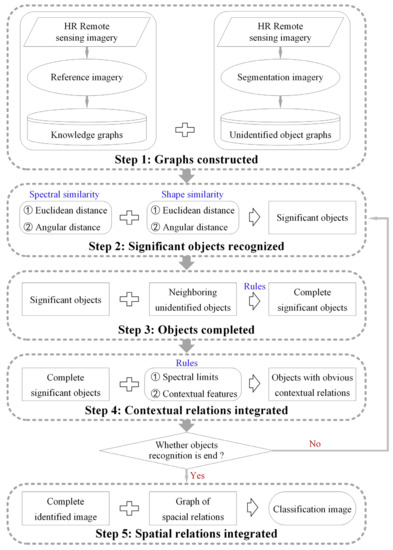
Figure 2.
Flowchart of the proposed classification method.
2.1. Knowledge Graph Construction
Due to the advantage of storing large ontologies and relationships in the knowledge graph [24,25], we can construct a knowledge repository simulating the human brain to better understand the world [26]. However, unlike the extraordinarily large amount of data from various fields stored in the human brain, the knowledge graph built in this study is smaller in size and specific to the field of HR remote sensing. Figure 3 depicts the process of knowledge graph construction. There are three steps for knowledge graph construction:
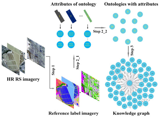
Figure 3.
Process of knowledge graph construction. HR RS imagery represents high resolution remote sensing imagery. Step 1, Step 2_1, Step 2_2, and Step 3 are the construction of the reference image, attribute extraction, ontology establishment, and integration of spatial relationships, respectively. The 1, 2, …, n in ontologies and attributes are the unique identifiers assigned to each image object, while the 1, 2, …, n in the knowledge graph represent each ontology.
- (1)
- Construction of the reference image (Step 1 in Figure 3): The reference image contains the category and contour of each real ground object, which is critical for extracting the objects and object features needed to construct a knowledge graph. Certain GIS software was applied to delineate vector objects and convert the original imagery to reference imagery. Three experts with several years of experience in the interpretation of objects in remote sensing imagery took two weeks to delineate nearly 100 HR remote sensing images for the construction of the reference image in this study.
- (2)
- Attribute extraction (Step 2_1 in Figure 3) and ontology establishment (Step 2_2 in Figure 3): An object and a feature of the object in the reference image correspond to an ontology and an attribute in the knowledge graph, respectively. Ontologies were established by assigning a unique identity to each object within the reference image, while the attributes of the ontology were obtained by extracting object features. The object features used in this study mainly include spectral features and shape features, of which the spectral features involve red, green, blue, and near-infrared band values and combinations of band indices of the remote sensing image, whereas shape features correspond to the area, perimeter, bar coefficient, etc. Table 1 depicts the detailed description of the object features.
- (3)
- Integration of spatial relationships (Step 3 in Figure 3): It is essential to consider the strong spatial relationships between adjacent objects in the reference image for subsequent classification. Relationships between the objects and their neighbors were separated into three categories in this work: adjacent, containing, and inside. Figure 4 illustrates these relationship categories. Each relationship is a direct line of connection in the knowledge graph. Therefore, by integrating all the ontologies and their direct connecting lines, the knowledge graph of a specific HR remote sensing image can be constructed. NEO4j was used as a knowledge graph database in this study. Unlike conventional databases that store data in tables, NEO4j is a graphic database that stores data in terms of nodes and node relationships. This provides a visual graphical interface and a specific data query language, which allows it to manage data more naturally and rapidly respond to queries while offering deeper context for analytics. The graphic storage and data processing capabilities of NEO4j ensure high data readability and integrity [27].
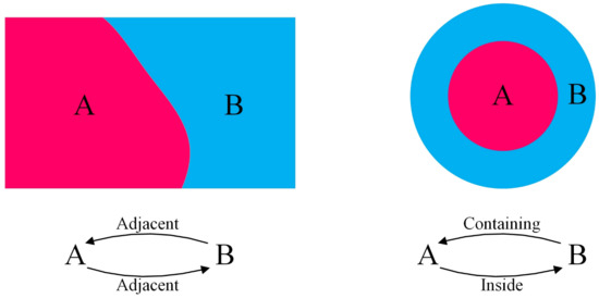 Figure 4. Diagram of the spatial relationships between neighboring objects. A and B represent different land covers. There are three types of relationships between objects: containing, inside, and adjacent.

Table 1.
Object features and their descriptions.
Table 1.
Object features and their descriptions.
| Features Type | Features | Description |
|---|---|---|
| Spectral | Red | Object pixels values that average in the red band |
| Green | Object pixels values that average in the green band | |
| Blue | Object pixels values that average in the blue band | |
| Near-infrared | Object pixels values that average in the near-infrared band | |
| NDWI | ||
| NDVI | ||
| Shape | Area (A) | Area of object |
| Perimeter (P) | Perimeter of object | |
| Long Axis Length (LAL) | Long axis length of the minimum outer rectangle of the object | |
| Short Axis Length (SAL) | Short axis length of the minimum outer rectangle of the object | |
| Principal Direction (PD) | The angle between the direction of the long axis and 0° of the object | |
| Rectangularity (R) | ||
| Elongation (E) | ||
| Bar (B) |
2.2. Image Segmentation and Unidentified Object Graph Construction
To facilitate the matching and inference of segmented objects, an unidentified object graph with the same data storage structure as the knowledge graph must be created. The process of constructing an unidentified object graph is comparable to that of a knowledge graph, except that a knowledge graph requires building reference imagery to obtain objects, while the unidentified object graph was supplied objects by image segmentation. Therefore, the effectiveness of the segmentation algorithm is crucial for subsequent classification. In this study, an unsupervised multiscale segmentation optimization (UMSO) method proposed by [23] was utilized as the segmentation algorithm for HR remote sensing imagery. This algorithm produced most of the objects similar in size and shape to actual objects on the ground (e.g., aquaculture pond, bare farmland, crop farmland, and road), while a few oversegmented objects were much smaller than the actual objects (e.g., embankment), which greatly reduced the error rate of subsequent object matching and the complexity of the proposed method.
UMSO was proposed based on a region-based multiscale segmentation (MSeg) algorithm, which initially generates oversegmentation results to obtain the segmentation results by merging smaller segmentation objects according to the scale parameters given by the user [28]. However, UMSO defines an optimal scale selection function via the process of merging MSeg objects for each image object, and then the optimal segmentation result of the image is derived by fusing each optimal segmentation object. The formula for the optimal scale selection function is as follows:
where is the scale parameter and . is the largest scale parameter for the segmentation. represents the interheterogeneity of object , and represents the intratumor heterogeneity of object . When increases to the highest value, object reaches the optimal segmentation scale.
As UMSO produces an optimal scale segmentation result for each object, the majority of objects in the segmentation result are closely with the real ground objects. The novel classification method proposed in our work relies on the matching of reference objects with segmentation objects. Therefore, the optimal scale segmentation of UMSO greatly enhanced the recognition accuracy of the proposed method and reduced the complication of merging segmentation objects.
2.3. Significant Objects Recognized
Since the unidentified object graph and the knowledge graph have been established, the remaining task is to match the unidentified objects in the unidentified object graph with the reference objects of the knowledge graph. Theoretically, as long as the segmentation objects are close enough to the actual ground object, we can successfully exploit a one-to-one matching scheme between the reference objects and the unidentified object. However, due to the complexity of the reflectance of ground objects in remote sensing imagery, no algorithm can achieve perfect image segmentation. Therefore, a hierarchy of identification approaches has been presented in this study. At the top of hierarchy are the unidentified objects with significant features in the image (significant objects). These are followed by the recognition of other insignificant unidentified objects. These significant objects with more prominent spectral features or shape features are easier to recognize. According to our experimental validation, objects with area > , rectangularity > , NDWI > , and NDVI > were relatively easy to identify directly by object matching; thus, they are considered significant objects for priority matching and recognition. Furthermore, to successfully match the significant objects, two distances (the angular distance and Euclidean distance) between the reference objects and the unidentified objects have been introduced to calculate the object similarity, which is usually utilized to calculate the similarity between two vectors [29,30,31]. The spectral and shape attributes for each object of the knowledge graph and the unidentified object graph, constitute a spectral vector and a shape vector , respectively. Thus, angular distance is used to measure the directional difference between vectors, while Euclidean distance measures the size difference between vectors. Then, the spectral and shape distances between the unidentified object and the reference object can be calculated:
where represents the spectral distance or shape distance between and . is the Euclidean distance and is the angular distance. Both and have been normalized. represents weight. is the component of a spectral vector or shape vector of the unidentified object, and corresponds to the component of a spectral vector or shape vector of the reference object. symbolizes the length of the vector. Using the spectral and shape distances, the similarity between the unidentified object and the reference object can be defined as:
where represents the spectral distance between and and represents the shape distance between and . Both and have been normalized. is the weight. Smaller values indicate increased similarity between the two objects.
Furthermore, in our matching process, which involves each object of the unidentified graph being compared to each object of the knowledge graph, a match was considered successful when the similarity between two objects reaches a minimum and the two objects are assigned the same class. However, such a matching method is overly general and easily produces false matches, even leading to misclassifications. As an example, when an unidentified object matches reference object and reference object , if = and < , might be identified as . In reality, however, the priority of spectral similarity exceeds shape similarity for the two objects of the same class; thus, should be of the same class as , rather than . Thus, the above situation would inevitably produce misclassifications. To solve this issue, a two-step matching approach has been proposed in this study to reduce this error. First, the spectral distances between the unidentified object and all reference objects were ranked in ascending order, and the top 5% of reference objects of the spectral distances were selected as candidate objects. Second, formula 5 was used to calculate the similarity between the unidentified object and these top 5% reference objects were used to identify the closest match among the reference objects. Figure 5 displays this process. Multiple experimental results demonstrated that such an approach can largely eliminate the errors caused by shape dependence and improve the matching efficiency.
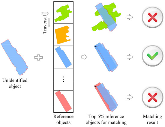
Figure 5.
The matching process for significant objects. There are two forms: shape matching and spectral matching, which are represented by the shapes and colors of objects in the figure, respectively. √ indicates successful matching, while × indicates failed matching.
2.4. Significant Object Completion
Although UMSO produces most of the segmented objects that are closer to the actual ground objects, there are unavoidably a few oversegmentation issues. Merging objects with neighboring objects to complete the significant objects can address this issue effectively and produce a result nearer to the actual ground objects. A rule named the principle of least similarity merging was defined for completing the significant object. For example, for an identified significant object , all similarities between the object merged by with its neighboring object and reference object must be calculated. When the of the merged object has decreased compared to the value of the original significant object and the minimum similarity value among all the calculated combinations has been identified, then the neighboring object was determined to be object that needs to be merged with . Thus, and this neighboring object were merged into one object . The process then iterates until all objects that satisfy the condition were merged. Figure 6 illustrates a schematic view of object merging, while Algorithm S1 details the specific process of object merging.
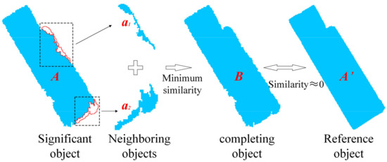
Figure 6.
Process of significant object completion. ,
and represent the identified significant
object, merged completing object, and reference object, respectively, while and are neighboring
objects of the identified significant object. The similarity in the figure is calculated from formula
5.
2.5. Integrating Contextual Relationships
The biggest preference for using a knowledge graph for classification is that it can explore the various relationships between objects, which enables the proposed method to apply logical reasoning ability to effectively deal with smaller oversegmented objects that are quite difficult to recognize. For example, when we classified a coastal zone image, the embankments around aquaculture ponds are usually segmented by the UMSO algorithm into numerous tiny objects adjacent to each other because of their narrow shape and unremarkable spectral reflectance. Misclassification often occurs if we follow the process described in Section 2.2 and Section 2.3 for embankment object matching. Therefore, the addition of contextual relationships can adequately recognize these objects. Based on years of expert experience in remote sensing image interpretation and the relationships between ground objects in actual remote sensing images, we derived a contextual relationship: aquaculture ponds are always surrounded by embankments. Thus, unidentified contiguous adjacent tiny objects around the aquaculture ponds were recognized as embankments when they are close enough in spectrum to the embankment objects of the reference image.
By following the steps of object matching, object completion, and contextual relationship integration, the majority of objects in the segmentation image were recognized. For the remaining unidentified objects, we lowered the discriminative conditions of significant objects and then repeated the process iteratively until all objects were fully recognized.
2.6. Integrating Spatial Relationships
Although steps 2 to 4 in Figure 2 have achieved relatively effective classification results for HR remote sensing imagery, there are still misclassifications. Using the spatial relationships contained in the reference imagery, many misclassified objects can be adjusted accordingly. Two graphs showing the spatial relationship between objects in the reference image and segmentation image were extracted based on the types of spatial relationships described in Section 2.1. Theoretically, the objects connected by each corresponding relationship in the two spatial graphs should be the same, which was interpreted in this study as being the same class. Therefore, the classification results were checked to adjust the misclassifications by comparing each corresponding relationship in the two spatial relation graphs.
Figure 7 depicts the process of comparing the spatial relationships using two graphs and Figure 8 depicts the process of integrating all the spatial relationships.
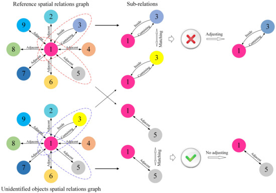
Figure 7.
Process of comparing two spatial relation graphs. The colors represent the classes of objects, while the edges represent the spatial relationships between objects in the figure. √ indicates successful matching, while × indicates failed matching.
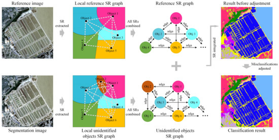
Figure 8.
Process of integrating all spatial relationships. The SR represents the spatial relation and Obj represents the object.
2.7. Quality Assessment
To reflect the performance of our proposed method, a pixel-based accuracy calculation assessment method was performed. All ground object classes in the reference image were considered positive classes, while the classes in the final classification image of the proposed method were predicted classes. A positive class may be predicted as positive (TP) or negative (FN). A negative class can likewise be predicted as being positive (FP) or negative (TN). Their combined indices included precision (also known as producer accuracy), Recall (also known as user accuracy), F1-score (F1), overall accuracy (OA), and kappa coefficient (Kappa), which were exploited to evaluate the final classification effectiveness. Precision, Recall, F1-score, OA, and Kappa are often utilized to calculate the accuracy of the classification [32,33], whose calculation formulas are as follows:
where , represents the number of ground object classes in a certain remote sensing image, is the number of samples in each class of the reference class, and corresponds to the number of samples in each class of the prediction class.
Precision represents the ratio of the number of samples correctly predicted as positive to the total number of samples predicted as positive. Recall represents the ratio of the number of samples correctly predicted as positive to the number of all positive samples. F1 is the average of the reconciliation of Precision and Recall. OA represents the ratio of the number of correctly predicted samples to the number of all predicted samples. Kappa is a classification consistency test based on the confusion matrix, and its value can represent the level of classification accuracy to a certain extent. Usually, higher values of Precision, Recall, F1-score, OA, and Kappa indicate higher classification accuracies.
3. Experimental Results
3.1. Experimental Data and Setup
The QuickBird-2 satellite was used as the source of experimental data in this study. QuickBird-2, with a 1.5-m ground sampling distance (GSD) resolution at an interval of 1.5 days, is an Earth-imaging satellite launched in October 2001 and operated by Maxar in the United States. The multispectral imagery produced by the QuickBird-2 satellite has a 2.4–2.6 m (GSD) spatial resolution and consists of four bands: blue, green, red, and NIR. Three multispectral images taken on 28 June 2008, from the QuickBird-2 satellite were utilized to assess the performance of the proposed classification method. The experimental area designated for this study is located in Qingdao, Shandong Province, which is a coastal city with a variety of geological landscapes. As shown in Figure 9a, the experimental area (Scenes A, B, and C) contains abundant land cover types, such as the sea, coastal aquaculture ponds, vegetation, buildings, farmland, etc. Scenes A, B, and C have sizes of 700 × 700 pixels, 600 × 600 pixels, and 500 × 500 pixels, respectively.
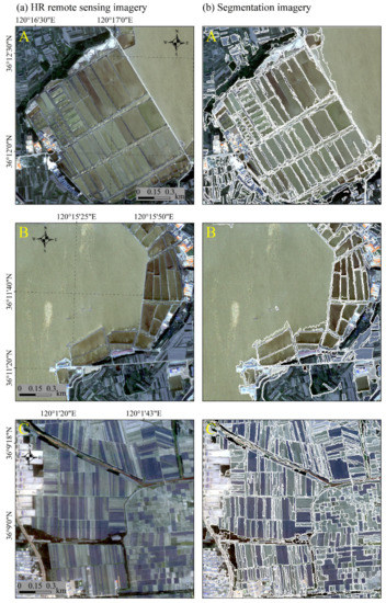
Figure 9.
Experimental imagery and segmentation imagery produced by the UMSO algorithm.
The segmentation method, UMSO, was applied in this study using MATLAB 2018b on a computer with an AMD R5-5600× CPU (3.7 GHz) and 32 G RAM. For consistency, the shape and compactness parameters required in the UMSO were set at 0.4 and 0.5, and the scale parameter was increased from 10 to 400 in increments of 10. In addition, according to repeated experiments, the weights for scenes A, B, and C in the classification process of the proposed method were all assigned a value of 0.5, while the weights were assigned 0.8, 0.6, and 0.75, respectively. The proposed novel classification method explained in Section 2 was run in Anaconda 3 on the same machine that runs Python 3.8.
3.2. Details of Knowledge Graph Construction
The knowledge graphs and unidentified object graphs were stored in the NEO4j database with ontologies, attributes, and relationships. Unidentified object graphs , , and and knowledge graphs , , and were constructed for scenes , , and , respectively. In summary, 2367 ontologies and 10,416 relationships were established, of which comprised 669 ontologies and 2927 relationships, comprised 341 ontologies and 1202 relationships, comprised 198 ontologies and 876 relationships, comprised 85 ontologies and 261 relationships, comprised 659 ontologies and 3097 relationships, and comprised 415 ontologies and 2053 relationships. Moreover, the relationships are further divided into adjacent, containing, and inside categories. Table 2 shows the details of the knowledge graph and the unidentified object graph.

Table 2.
Detailed information about ontologies and relationships in the knowledge graph and the unidentified object graph. A, B, C, , and represent the knowledge graphs and the unidentified object graphs over experimental scenes A, B, and C, respectively.
3.3. Details of the Classification Process
The proposed method, as mentioned in Section 2, was applied to the experimental scenes, and the experimental imagery was first segmented, as shown in Figure 9b. Then, the classification imagery was generated by recognizing and completing the significant objects and contextualizing and integrating the spatial relationships. Taking scene A as an example, we present the results obtained in each step of scene A processing, as shown in Figure 10, where Figure 10c–e, and f represent the recognition, completion, contextualization, and integration (or final classification), respectively. Significant changes in the results of each before and after processing step are indicated by dashed boxes of different colors in Figure 10. For example, the red dashed boxes and the black dashed boxes represent the significantly advanced parts of the classification results after significant object completion and spatial relation integration, respectively.
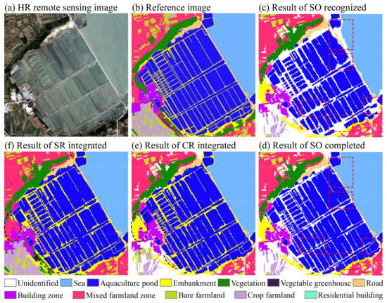
Figure 10.
Results of each processing step of scene A. The HR, SO, CR, and SR represent high resolution, significant objects, contextual relationships, and spatial relationships, respectively. Different background colors in the imagery represent different land covers. Dashed boxes in different colors represent the significant change areas from the previous result to the next result.
3.4. Classification Result Evaluated
The confusion matrices (Figure 11a,c,e) were utilized to calculate the TP, TN, FP, and FN of the classification results. Figure 11a,c,e depicts the results for scenes A, B, and C, respectively. TP was represented by the diagonal lines of the confusion matrix. FP was represented as the sum of all elements in a column of the confusion matrix subtracted from the TP of this column. FN was represented as the sum of all elements in a row of the confusion matrix subtracted from the TP of this row. TN was represented as the sum of all elements of the confusion matrix subtracted from (TP+ FP + FN). Therefore, the Precision, Recall, F1-score, overall accuracy of the classification results, and kappa coefficients calculated for each class of ground objects in scenes A, B, and C are displayed in Figure 11b,d,f, respectively.
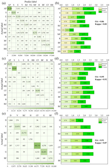
Figure 11.
Confusion matrices and evaluation indices calculated over experimental scenes. (a,c,e) are the confusion matrices for scenes A, B, and C, respectively. (b,d,f) are the calculation results of the evaluation indices for scenes A, B, and C, respectively. The AP, S, E, V, BZ, VG, MF, R, BF, CF, RB, L, B, D, H, and G represent aquaculture pond, sea, embankment, vegetation, building zone, vegetable greenhouse, mixed farmland zone, road, bare farmland, crop farmland, residential building, lawn, boat, ditch, highway, and grassland, respectively.
Overall, the classification results were satisfactory, with the overall accuracy of scenes A, B, and C all exceeding 85%. According to [34], Kappa values from 0.00 to 0.20 are only somewhat consistent, 0.21 to 0.40 are fairly consistent, 0.41 to 0.60 are moderately consistent, 0.61 to 0.80 are substantially consistent, and 0.81 to 1.00 are almost perfect. Notably, the Kappa of our proposed method exceeded 0.82 in the classification results of all three scenes, indicating that the classification effectiveness of the proposed method is considerable. Figure 12 exhibits the comparison of the reference imagery and classification results. For visual performance, obviously the reference imagery and the classification results are almost consistent in the three scenes. The overall classification presentation of the proposed method was more in line with our expectations.
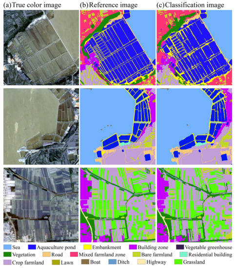
Figure 12.
Comparison of the classification result and reference image. (a) is the true color imagery of the original HR remote sensing imagery. The background colors in (b,c) represent different land covers.
Specifically, the recognition effect of out proposed method performed best on large ground objects with prominent and more obvious features, while it performed less well on smaller ground objects with irregular shapes. For example, the classification results for aquaculture ponds, sea, farmland, building zones, and roads with larger areas, larger rectangularity, and more prominent spectral features in scenes A, B, and C were nearly consistent with the ground objects in the reference image (Figure 12b,c). In particular, for the recognition of aquaculture ponds, sea areas, and building zones, the Precisions, Recalls, and F1-scores of aquaculture ponds and sea in scene A were 0.96, 0.92, 0.94, and 1.00, 0.99, 1.00, respectively (Figure 11b). The precisions, recalls, and F1-scores for aquaculture ponds and sea areas in scene B also exceeded 0.94 (Figure 11d). The recognition accuracy of the building zone in scene C was also extremely high, with Precision, Recall, and F1-score all close to approximately 0.94 (Figure 11f). In addition, apart from the high recognition accuracy of the abovementioned ground objects, there were also many other ground objects with relatively good recognition results, such as roads and crop farmland in scene A, residential buildings and crop farmland in scene B, and vegetation, highways, and crop farmland in scene C (Figure 11b,d,f). Sensitivity to significant ground objects was the main contribution to object matching using knowledge graphs, which is consistent with the process of prioritizing significant targets when our own brains recognize real ground objects. Such a classification is consistent with our perception of visual interpretation, and its recognition effect is also acceptable to researchers.
However, for several aspects, our classification results were not perfect. A large number of oversegmented objects will be generated during the segmentation process, which do not have an exact matching object in the knowledge graph. Therefore, these object classifications cannot be matched exactly but need to be fuzzy matched through the “minimum distance matching principle” (i.e., if an unidentified object has the smallest distance from a reference object of the knowledge graph, then it is assigned the class of the reference object) or via their contextual and spatial relationships. Although most objects can be accurately identified through the integration of contextual and spatial relationships, as well as spectral and shape rules, there were still misclassifications. This situation was particularly prominent in ground objects that are small in size or thin and narrow in shape. As an example, the Precision, Recall, and F1-score of the greenhouse in scene A are all only 0.36 (Figure 11b). The reason for the low recognition accuracy of the greenhouse is the small area and the less prominent spectral and shape features. The accuracy of the embankment classification in scene A, (as measured by Precision, Recall, and F1-score, which are 0.60, 0.77, and 0.67, respectively) was also not high. This was mainly due to the serious oversegmentation. Therefore, the proposed novel classification method can achieve higher accuracy if the accuracy of the previous segmentation method is advanced.
4. Discussion
4.1. Comparison with Other Methods
To evaluate the classification performance of the proposed method, the object-based KNN, SVM, DT, and RF methods [13,14,16,35,36] were compared with the proposed method. Table 3, Table 4, Table 5 and Table 6 report the details of the classification methods applied to experimental scenes. Three basic indices are shown in tables, including the harmonic score of Precision and Recall (F1-score), overall accuracy (OA), and kappa coefficient (Kappa). From the tables, we can observe that the proposed method had the highest OA and Kappa among the five methods (Table 3), which indicates that the proposed method had the best overall classification performance. For the identification of each class, the number of times that the proposed method reached the highest F1-score is significantly higher than the other four methods, with 6, 9, and 4 times for scenes A, B, and C, accounting for 55%, 90%, and 57% of the total number of highest F1 scores, respectively (Table 4, Table 5 and Table 6). SVM, DT, and RF, which are highly popular classification methods, have also shown potential use in classification tasks [14,37,38,39]. This is especially true for the RF and SVM methods in scene A. At 0.86, the OA of RF was the same as that of the proposed method (Table 3), while SVM attained the highest F1 score 4 times, second only to the 6 times reached by the proposed method (Table 4). In contrast, the performance of the KNN method was unremarkable. In addition, from the tables, we also see that the classification accuracy of the proposed method was significantly higher than that of other methods on significant ground objects, such as building zones, roads, and crop farmland (Table 4, Table 5 and Table 6), while the accuracy of ground objects with smaller areas, such as greenhouses, was lower than other methods (Table 4). The main reason was that the segmentation algorithm proposed by [40] was utilized in KNN, SVM, DT, and RF, which can still produce oversegmented objects for smaller ground objects, while the UMSO segmentation algorithm used in the proposed method tends to produce undersegmented objects for these smaller objects, thus making it easy to classify these objects into the backgrounds in the process.

Table 3.
Comparison of OAs and Kappas using the KNN, SVM, DT, RF, and proposed methods for experimental scenes A, B, and C. Bold represents the highest precision of a same class among these methods.

Table 4.
Comparison of F1 scores using the KNN, SVM, DT, RF, and proposed methods for experimental scene A. Bold represents the highest precision of a same class among these methods.

Table 5.
Comparison of F1 scores using the KNN, SVM, DT, RF, and proposed methods for experimental scene B. Bold represents the highest precision of a same class among these methods.

Table 6.
Comparison of F1 scores using the KNN, SVM, DT, RF, and proposed methods for experimental scene C. Bold represents the highest precision of a same class among these methods.
Figure 13 shows the comparison of the results of the KNN, SVM, DT, RF, and proposed methods. To better visualize the differences between the results of the five methods and the reference image, we divided the misclassified results into false negatives (FN) and false positives (FP), and the results are presented in Figure 13. Overall, we can observe that the FNs and FPs of the proposed method, DT, and RF were significantly less than those of the KNN and SVM methods. Moreover, the FNs and FPs of KNN and SVM appeared in various regions, while those values were concentrated within a small region of the imagery in the other three methods. This was especially true for the proposed method, which was the closest to the reference image with the fewest FNs and FPs (Figure 13), indicating that KNN and SVM may often misclassify ground objects more frequently than the other three methods. Specifically, the proposed method had significant advantages in object integrity extraction, especially for ground objects such as aquaculture ponds and sea areas with salient features while the objects extracted by KNN and SVM often had relatively obvious salt and pepper noise. Notably, DT and RF had the same classification performance as the proposed method due to their excellent classification ability. However, due their insensitivity to smaller objects, some detailed information will inevitably be lost in the classification process of the proposed method. For example, for the bare farmland in scene A, because of its spectral proximity to the surrounding mixed farmland zone, the UMSO algorithm easily segments the two into the same object, which will lead to the loss of classification details.
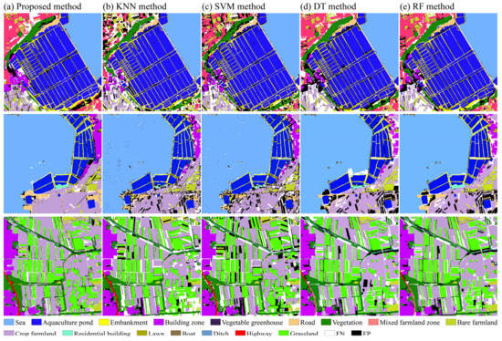
Figure 13.
Comparison of the proposed method with the KNN, SVM, DT, and RF methods. Different background colors in the imagery represent different land cover types. The FN and FP represent two types of misclassification results: false negative and false positive.
4.2. Expectations
Knowledge graphs play a crucial role in the proposed method, which, similar to the human brain, provides a reference knowledge base for humans to understand the objective world. Although the knowledge graph constructed in our work was only for a specific remote sensing scene, the proposed method has universal applicability. When the constructed knowledge graph was applied to other remote sensing image scenes with similar ground objects, it could also achieve a consistent classification result. Taking our experimental scenes as an example, scenes A and B have similar ground objects, and the knowledge graph constructed in scene A was used to classify scene B to demonstrate the universality of the proposed method. The final result is shown in Figure 14. We can observe that scenes A and B have similar classes, such as aquaculture ponds, sea, bare farmland, and roads (Figure 12a). Therefore, applying the knowledge graph constructed in scene A to execute fuzzy matching, object completion, and contextualization and the integration of spatial relationships on scene B can derive comparable classification results as using the knowledge graph constructed in scene B for classification. Due to the lack of accurate reference objects, some misclassifications will inevitably occur, as shown by the red elliptical dashed line in Figure 14. Since the unidentified object cannot match the exact object in the knowledge graph in scene A, the reference object with the smallest distance is matched according to the “minimum distance matching principle” proposed in Section 3.3. However, because the spectra of certain two classes of objects in scene A were similar, such as roads and embankments, the road in scene B was easily misclassified as an embankment (Figure 14). Of course, such a situation can be adjusted by controlling the similarity of the matching results. For example, if the similarity is greater than a certain threshold , we consider the matching to have failed and abandon this matching. Overall, our proposed method is scalable. When the established knowledge graph contains enough knowledge, achieving high accuracy recognition is quite possible. For example, if OpenStreetMap and the corresponding HR remote sensing imagery are applied to construct a large-scale remote sensing knowledge graph, combined with our proposed method, the classification task of most remote sensing image scenes can be realized, which is the primary focus of our future research.
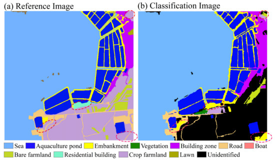
Figure 14.
Results of using the knowledge graph in scene A to classify scene B. Different background colors in the imagery represent different land covers.
The segmentation algorithm is also one of the most important components of the proposed classification method. Although UMSO produced most of the segmented objects (over 60% of the total) that are close to the real ground object in both size and shape, some oversegmented objects were produced that are much smaller than the real ground objects, or undersegmented objects were produced that are much larger than the real ground object. This will increase the misclassification rate of the results. To date, many multiscale segmentation optimization algorithms have been proposed, such as [41,42,43]. One of the main goals of our future work is to combine the method proposed in our work with different multiscale segmentation optimization algorithms and then comparing the results to achieve the best classification. Alternatively, we expect to establish a new multiscale segmentation optimization algorithm that is most suitable for the proposed method.
5. Conclusions
The use of knowledge graphs in the classification of remote sensing imagery is a highly regarded and challenging task in GEOBIA. In this study, a knowledge graph-based classification method was proposed for HR remote sensing imagery. Using the reference image and UMSO segmentation algorithm, the knowledge graph and the unidentified object graph corresponding to the specific remote sensing scene were constructed, respectively. Then, the recognition of significant objects was accomplished by calculating the similarity between the unidentified objects and the reference objects. Significant objects were completed by merging the identified significant objects and their surrounding unidentified objects. Contextual and spatial relationships were integrated to obtain a robust classification result. The proposed method has employed the capability of knowledge graphs to address many problems previously caused by disregarding object relationships. Furthermore, the combination of object matching and knowledge graphs has been proposed for the first time in our work and applied to HR remote sensing image classification, thus, providing a new idea for how to apply GEOBIA.
Three experimental HR images with different land covers, such as sea surfaces, aquaculture ponds, farmland, and buildings, were utilized to evaluate the classification accuracy. The results demonstrated that the proposed method was highly capable of identifying different landscapes. In the experimental scenes, the OAs of the proposed method all exceed 0.85, and the Kappas all exceed 0.82. Compared with the KNN, SVM, DT, and RF methods, both OA and Kappa of the proposed method were higher. Additionally, our method achieved the highest F1 score for landscapes more frequently than the other methods. However, lower classification accuracy results also occurred because the UMSO segmentation algorithm undersegments smaller objects. Overall, the proposed method can achieve satisfactory classification results. Furthermore, the proposed method is scalable and can be applied for the classification of different remote sensing imagery. In the future, we will optimize the performance of classification methods by improving the content of the knowledge graph and establishing a more suitable segmentation algorithm.
Supplementary Materials
The following supporting information can be downloaded at: https://www.mdpi.com/article/10.3390/rs15020321/s1, Algorithm S1. Significant object completion.
Author Contributions
Conceptualization, J.C. and Z.G.; methodology, J.C. and Z.G.; data analysis, J.C. and Z.G.; investigation, J.C. and Z.G.; resources, J.C. and Z.G.; writing, Z.G.; supervision, J.C.; project administration, J.C.; funding acquisition, J.C. All authors have read and agreed to the published version of the manuscript.
Funding
This research was funded by the NSFC-Zhejiang Joint Fund for the Integration of Industrialization and Informatization (Grant No. U1609202), and the National Natural Science Foundation of China (Grant Nos. 41376184 and 40976109).
Data Availability Statement
Not applicable.
Conflicts of Interest
The authors declare no conflict of interest.
References
- Zhu, Q.; Sun, X.; Zhong, Y.; Zhang, L. High-resolution remote sensing image scene understanding: A review. In Proceedings of the IGARSS 2019-2019 IEEE International Geoscience and Remote Sensing Symposium, Yokohama, Japan, 28 July–2 August 2019; pp. 3061–3064. [Google Scholar]
- Chan, R.H.; Ho, C.W.; Nikolova, M. Salt-and-pepper noise removal by median-type noise detectors and detail-preserving regularization. IEEE Trans. Image Process. 2005, 14, 1479–1485. [Google Scholar] [CrossRef]
- Ma, L.; Li, M.; Ma, X.; Cheng, L.; Du, P.; Liu, Y. A review of supervised object-based land-cover image classification. Isprs J. Photogramm. Remote Sens. 2017, 130, 277–293. [Google Scholar] [CrossRef]
- Janowski, L.; Tylmann, K.; Trzcinska, K.; Rudowski, S.; Tegowski, J. Exploration of glacial landforms by object-based image analysis and spectral parameters of digital elevation model. IEEE Trans. Geosci. Remote Sens. 2021, 60, 4502817. [Google Scholar] [CrossRef]
- Chen, G.; Weng, Q.; Hay, G.J.; He, Y. Geographic object-based image analysis (GEOBIA): Emerging trends and future opportunities. GIScience Remote Sens. 2018, 55, 159–182. [Google Scholar] [CrossRef]
- Kucharczyk, M.; Hay, G.J.; Ghaffarian, S.; Hugenholtz, C.H. Geographic object-based image analysis: A primer and future directions. Remote Sens. 2020, 12, 2012. [Google Scholar] [CrossRef]
- Aplin, P.; Smith, G. Advances in object-based image classification. Int. Arch.Photogramm. Remote Sens. Spat. Inf. Sci. 2008, 37, 725–728. [Google Scholar]
- Dronova, I. Object-based image analysis in wetland research: A review. Remote Sens. 2015, 7, 6380–6413. [Google Scholar] [CrossRef]
- Hossain, M.D.; Chen, D. Segmentation for Object-Based Image Analysis (OBIA): A review of algorithms and challenges from remote sensing perspective. ISPRS J. Photogramm. Remote Sens. 2019, 150, 115–134. [Google Scholar] [CrossRef]
- Li, M.; Zang, S.; Zhang, B.; Li, S.; Wu, C. A review of remote sensing image classification techniques: The role of spatio-contextual information. Eur. J. Remote Sens. 2014, 47, 389–411. [Google Scholar] [CrossRef]
- Martins, V.S.; Kaleita, A.L.; Gelder, B.K.; da Silveira, H.L.; Abe, C.A. Exploring multiscale object-based convolutional neural network (multi-OCNN) for remote sensing image classification at high spatial resolution. ISPRS J. Photogramm. Remote Sens. 2020, 168, 56–73. [Google Scholar] [CrossRef]
- Wahidin, N.; Siregar, V.P.; Nababan, B.; Jaya, I.; Wouthuyzen, S. Object-based image analysis for coral reef benthic habitat mapping with several classification algorithms. Procedia Environ. Sci. 2015, 24, 222–227. [Google Scholar] [CrossRef]
- Tu, B.; Wang, J.; Kang, X.; Zhang, G.; Ou, X.; Guo, L. KNN-based representation of superpixels for hyperspectral image classification. IEEE J. Sel. Top. Appl. Earth Obs. Remote Sens. 2018, 11, 4032–4047. [Google Scholar] [CrossRef]
- Charbuty, B.; Abdulazeez, A. Classification based on decision tree algorithm for machine learning. J. Appl. Sci. Technol. Trends 2021, 2, 20–28. [Google Scholar] [CrossRef]
- Belgiu, M.; Drăguţ, L. Random forest in remote sensing: A review of applications and future directions. ISPRS J. Photogramm. Remote Sens. 2016, 114, 24–31. [Google Scholar] [CrossRef]
- Chandra, M.A.; Bedi, S. Survey on SVM and their application in image classification. Int. J. Inf. Technol. 2021, 13, 1–11. [Google Scholar] [CrossRef]
- Chen, X.; Jia, S.; Xiang, Y. A review: Knowledge reasoning over knowledge graph. Expert Syst. Appl. 2020, 141, 112948. [Google Scholar] [CrossRef]
- Li, Y.; Kong, D.; Zhang, Y.; Tan, Y.; Chen, L. Robust deep alignment network with remote sensing knowledge graph for zero-shot and generalized zero-shot remote sensing image scene classification. ISPRS J. Photogramm. Remote Sens. 2021, 179, 145–158. [Google Scholar] [CrossRef]
- Pujara, J.; Miao, H.; Getoor, L.; Cohen, W. Knowledge graph identification. In Proceedings of the International Semantic Web Conference, Sydney, NSW, Australia, 21–25 October 2013; pp. 542–557. [Google Scholar]
- Zhang, D.; Cui, M.; Yang, Y.; Yang, P.; Xie, C.; Liu, D.; Yu, B.; Chen, Z. Knowledge graph-based image classification refinement. IEEE Access 2019, 7, 57678–57690. [Google Scholar] [CrossRef]
- Tobler, W.R. A computer movie simulating urban growth in the Detroit region. Econ. Geogr. 1970, 46, 234–240. [Google Scholar] [CrossRef]
- Sun, S.; Dustdar, S.; Ranjan, R.; Morgan, G.; Dong, Y.; Wang, L. Remote Sensing Image Interpretation With Semantic Graph-Based Methods: A Survey. IEEE J. Sel. Top. Appl. Earth Obs. Remote Sens. 2022, 15, 4544–4558. [Google Scholar] [CrossRef]
- Shen, Y.; Chen, J.; Xiao, L.; Pan, D. Optimizing multiscale segmentation with local spectral heterogeneity measure for high resolution remote sensing images. ISPRS J. Photogramm. Remote Sens. 2019, 157, 13–25. [Google Scholar] [CrossRef]
- Rizun, M. Knowledge graph application in education: A literature review. Acta Univ. Lodz. Folia Oeconomica 2019, 3, 7–19. [Google Scholar] [CrossRef]
- Tchechmedjiev, A.; Fafalios, P.; Boland, K.; Gasquet, M.; Zloch, M.; Zapilko, B.; Dietze, S.; Todorov, K. ClaimsKG: A knowledge graph of fact-checked claims. In Proceedings of the International Semantic Web Conference, Auckland, New Zealand, 26–30 October 2019; pp. 309–324. [Google Scholar]
- Song, Y.; Li, A.; Tu, H.; Chen, K.; Li, C. A Novel Encoder-Decoder Knowledge Graph Completion Model for Robot Brain. Front. Neurorobotics 2021, 15, 674428. [Google Scholar] [CrossRef]
- Hao, X.; Ji, Z.; Li, X.; Yin, L.; Liu, L.; Sun, M.; Liu, Q.; Yang, R. Construction and Application of a Knowledge Graph. Remote Sens. 2021, 13, 2511. [Google Scholar] [CrossRef]
- Tzotsos, A.; Argialas, D. MSEG: A generic region-based multi-scale image segmentation algorithm for remote sensing imagery. In Proceedings of the ASPRS 2006 Annual Conference, Reno, Nevada, 1–5 May 2006; pp. 1–13. [Google Scholar]
- Senoussaoui, M.; Kenny, P.; Stafylakis, T.; Dumouchel, P. A Study of the Cosine Distance-Based Mean Shift for Telephone Speech Diarization. IEEE/ACM Trans. Audio Speech Lang. Process. 2014, 22, 217–227. [Google Scholar] [CrossRef]
- Choi, H.; Som, A.; Turaga, P. AMC-loss: Angular margin contrastive loss for improved explainability in image classification. In Proceedings of the IEEE/CVF Conference on Computer Vision and Pattern Recognition Workshops, Seattle, WA, USA, 14–19 June 2020; pp. 838–839. [Google Scholar]
- Yan, L.; Cui, M.; Prasad, S. Joint euclidean and angular distance-based embeddings for multisource image analysis. IEEE Geosci. Remote Sens. Lett. 2018, 15, 1110–1114. [Google Scholar] [CrossRef]
- Harjanti, T.W.; Setiyani, H.; Trianto, J.; Rahmanto, Y. Classification of Mint Leaf Types Based on the Image Using Euclidean Distance and K-Means Clustering with Shape and Texture Feature Extraction. Tech-E 2022, 5, 115–124. [Google Scholar]
- Nair, B.B.; Sakthivel, N. A Deep Learning-Based Upper Limb Rehabilitation Exercise Status Identification System. Arabian Journal for Science and Engineering 2022, 1–35. [Google Scholar] [CrossRef]
- Wan, T.; Jun, H.; Hui Zhang, P.W.; Hua, H. Kappa coefficient: A popular measure of rater agreement. Shanghai Arch. Psychiatry 2015, 27, 62. [Google Scholar]
- Phan, T.N.; Kuch, V.; Lehnert, L.W. Land Cover Classification using Google Earth Engine and Random Forest Classifier—The Role of Image Composition. Remote Sens. 2020, 12, 2411. [Google Scholar] [CrossRef]
- Wang, P.; Fan, E.; Wang, P. Comparative analysis of image classification algorithms based on traditional machine learning and deep learning. Pattern Recognit. Lett. 2021, 141, 61–67. [Google Scholar] [CrossRef]
- Cervantes, J.; Garcia-Lamont, F.; Rodríguez-Mazahua, L.; Lopez, A. A comprehensive survey on support vector machine classification: Applications, challenges and trends. Neurocomputing 2020, 408, 189–215. [Google Scholar] [CrossRef]
- Maulik, U.; Chakraborty, D. Remote Sensing Image Classification: A survey of support-vector-machine-based advanced techniques. IEEE Geosci. Remote Sens. Mag. 2017, 5, 33–52. [Google Scholar] [CrossRef]
- Zhang, Y.; Cao, G.; Li, X.; Wang, B. Cascaded random forest for hyperspectral image classification. IEEE J. Sel. Top. Appl. Earth Obs. Remote Sens. 2018, 11, 1082–1094. [Google Scholar] [CrossRef]
- Jin, X. A segmentation-based image processing system. U.S. Patent WO2009065021 A1[P], 22 May 2009. [Google Scholar]
- Chen, J.; Pan, D.; Mao, Z. Image-object detectable in multiscale analysis on high-resolution remotely sensed imagery. Int. J. Remote Sens. 2009, 30, 3585–3602. [Google Scholar] [CrossRef]
- Li, Y.; Feng, X. A multiscale image segmentation method. Pattern Recognit. 2016, 52, 332–345. [Google Scholar] [CrossRef]
- Du, S.; Du, S.; Liu, B.; Zhang, X. Context-enabled extraction of large-scale urban functional zones from very-high-resolution images: A multiscale segmentation approach. Remote Sens. 2019, 11, 1902. [Google Scholar] [CrossRef]
Disclaimer/Publisher’s Note: The statements, opinions and data contained in all publications are solely those of the individual author(s) and contributor(s) and not of MDPI and/or the editor(s). MDPI and/or the editor(s) disclaim responsibility for any injury to people or property resulting from any ideas, methods, instructions or products referred to in the content. |
© 2023 by the authors. Licensee MDPI, Basel, Switzerland. This article is an open access article distributed under the terms and conditions of the Creative Commons Attribution (CC BY) license (https://creativecommons.org/licenses/by/4.0/).