


Study on the Regeneration Probability of Understory Coniferous Saplings in the Liangshui Nature Reserve Based on Four Modeling Techniques

 , , , and
Abstract
: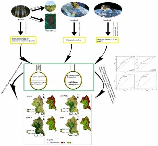
1. Introduction
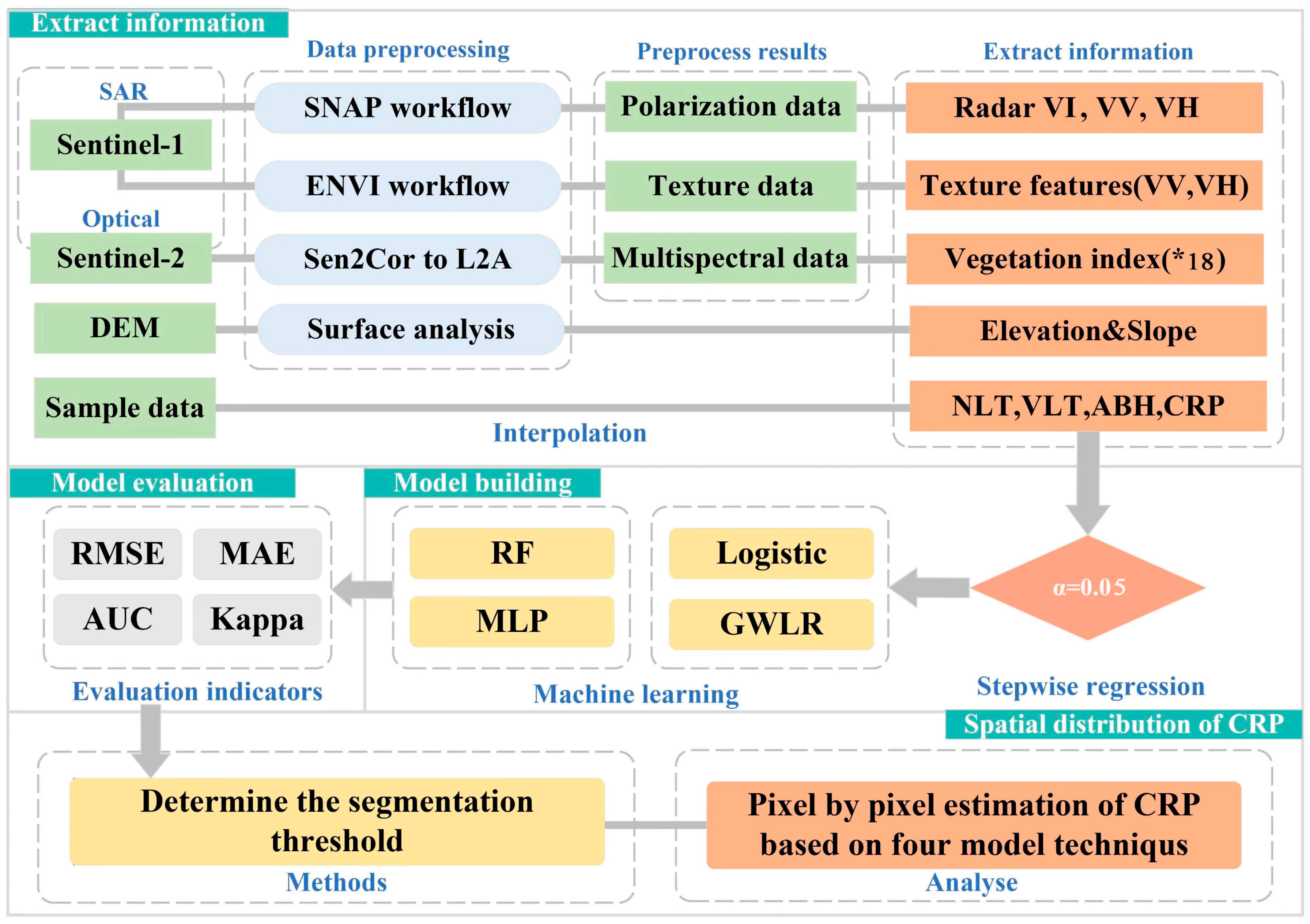
2. Materials and Methods
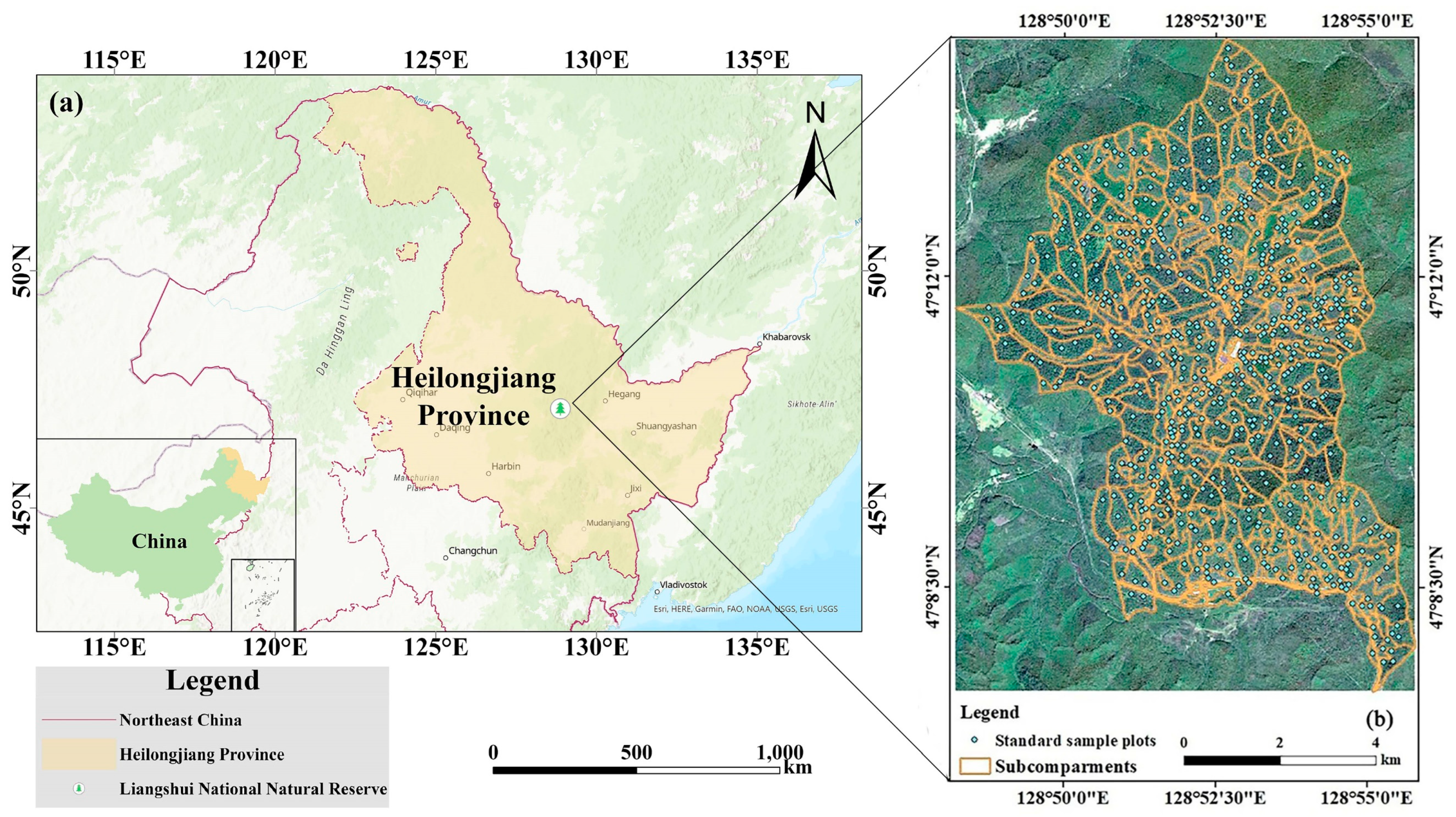
2.1. Overview of the Study Area
2.2. Data Acquisition
2.2.1. Ground Standard Land Survey
2.2.2. Remote Sensing Data Acquisition

| Vegetation Index | Abbreviation | Calculation Formula | |
|---|---|---|---|
| S2-VI | Ratio VI | RVI (S2) | B8/B4 [43] |
| Difference VI | DVI | B8–B4 | |
| Weighted Difference VI | WDVI | B8–0.5 × B4 | |
| Infrared Percentage VI | IPVI | B8/(B8 + B4) [44] | |
| Perpendicular VI | PVI | × B8–cos (45°) × B4 | |
| Normalized Difference VI | NDVI | (B8–B4)/(B8 + B4) | |
| Transformed Normalized Difference VI | TNDVI | [(B8–B4)/(B8 + B4) + 0.5]1/2 | |
| Soil-Adjusted VI | SAVI | 1.5 × (B8–B4)/8 × (B8 + B4 + 0.5) | |
| Modified Soil-Adjusted VI | MSAVI | (2–NDVI × WDVI) × (B8–B4)/8 × (B8 + B4 + 1–NDVI × WDVI) | |
| Modified Soil-Adjusted VI2 | MSAVI2 | 0.5 × (2 × (B8 + 1)) –sqrt [(2 × B8 + 1) × (2 × B8 + 1) –8 × (B8–B4)] | |
| Atmospheric Ratio VI | ARVI | [B8–(2 × B4–B2)]/[B8 + (2 × B4–B2)] | |
| Normalized Difference Water Index | NDWI | (B3–B8)/(B3 + B8) | |
| Normalized Difference Built-up Index | NDBI | (B11–B8)/(B11 + B8) | |
| Green Atmospherically Resistant Index | GARI | (B8–(B3–1.7 × (B2–B4)))/(B8 + (B3–1.7 × (B2–B4))) | |
| Optimized Soil-Adjusted VI | OSAVI | 1.5 × (B8–B4)/(B8 + B4 + 0.16) | |
| VI Green | VIG | (B3–B4)/(B3 + B4) | |
| Normalized Difference Moisture Index | NDMI | (B8–B11)/(B8 + B11) | |
| Normalized Difference Senescent VI | NDSVI | (B11–B4)/(B11 + B4) | |
| S1-Textural | Mean | VH_MEA VV_MEA | |
| Variance | VH_VAR VV_VAR | ||
| Homogeneity | VH_HOM VV_HOM | ||
| Contrast | VH_CON VV_CON | ||
| Dissimilarity | VH_DIS VV_DIS | ||
| Entropy | VH_ENT VV_ENT | ||
| Second Moment | VH_ASM VV_ASM | ||
| Correlation | VH_COR VV_COR | ||
| S1 | – | VV, VH | – |
| Radar VI | RVI (S1) | VH/VV | |
| DEM | DEM (m) | – | Composed of elevation values of points on the ground |
| Slope (°) | – | Rate of elevation change at a point on the ground |
2.2.3. Variable Screening
2.2.4. Study on CRP based on the LR Model
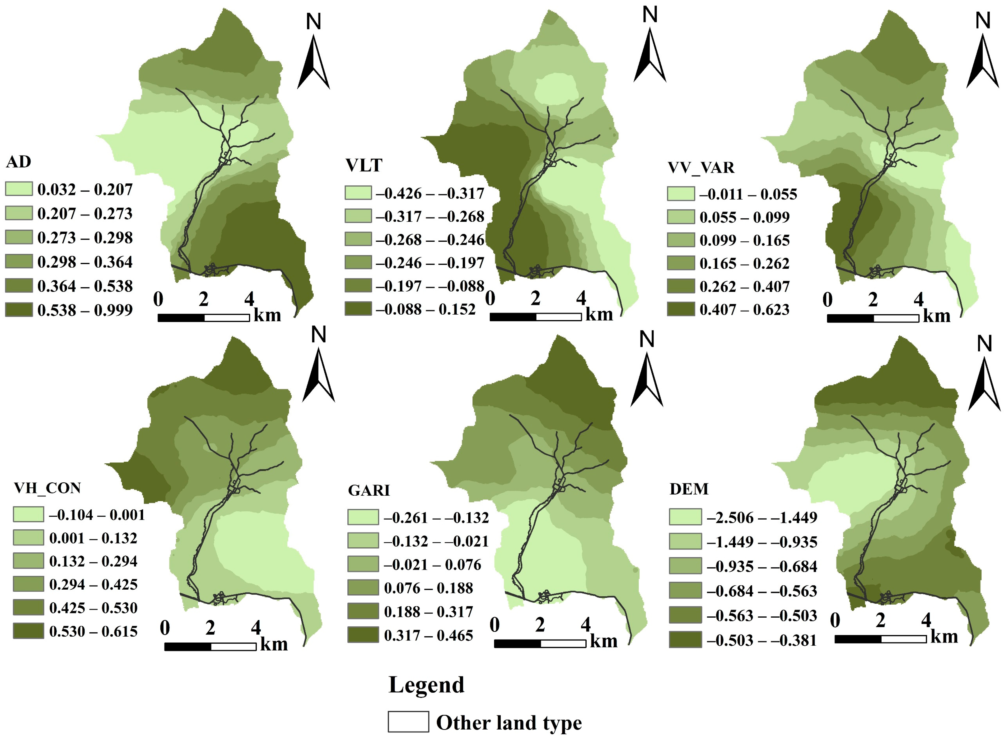
2.2.5. Study on CRP Based on the GWLR Model
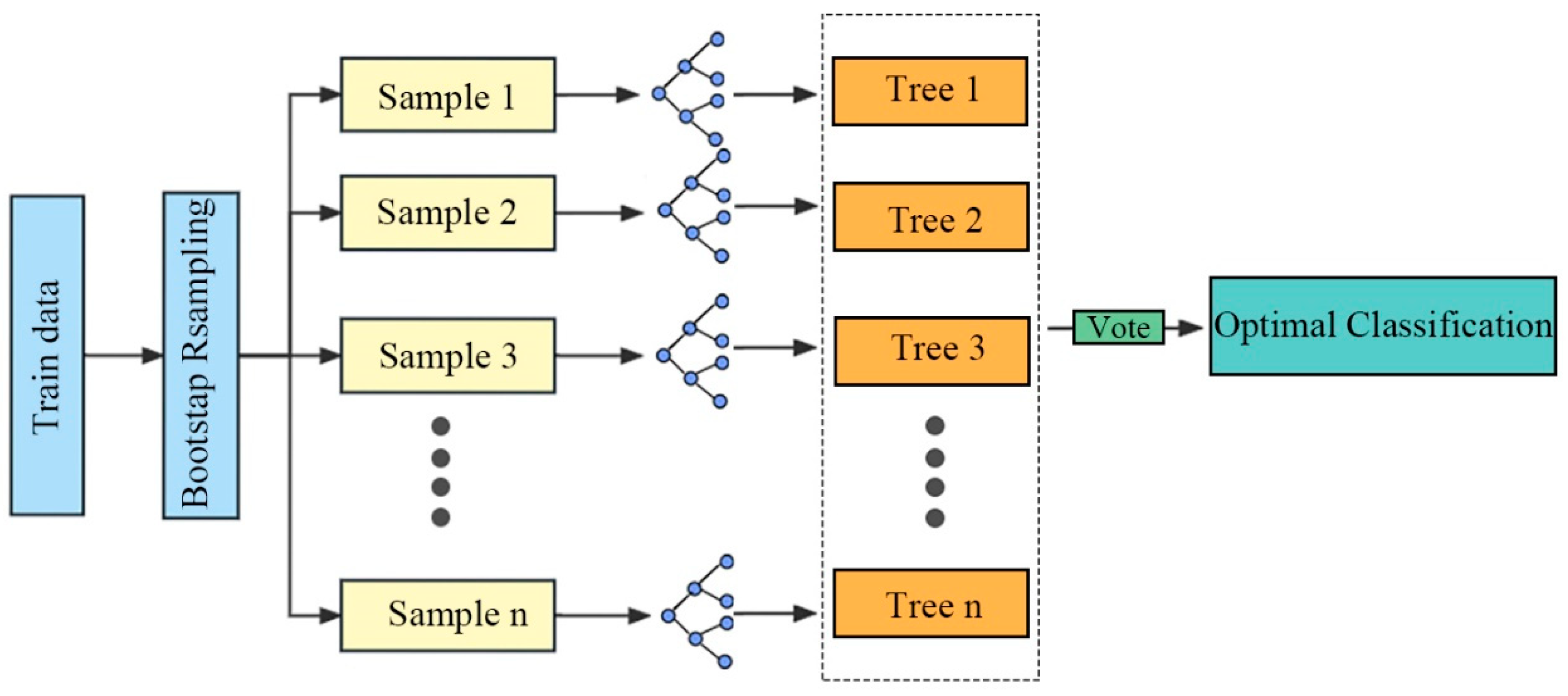
2.2.6. Study on CRP Based on the RF Model
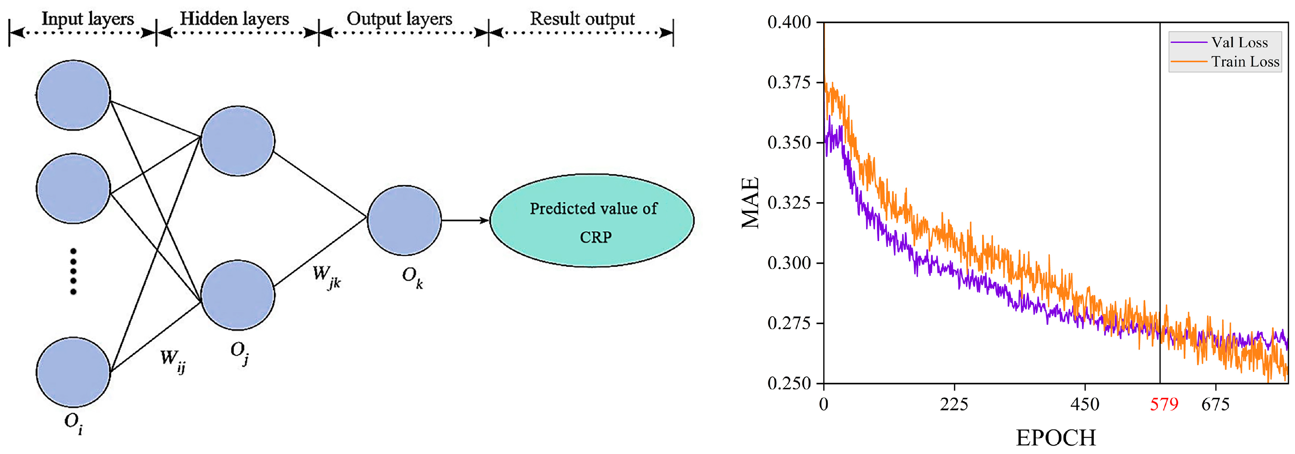
2.2.7. Study on CRP Based on the MLP Model
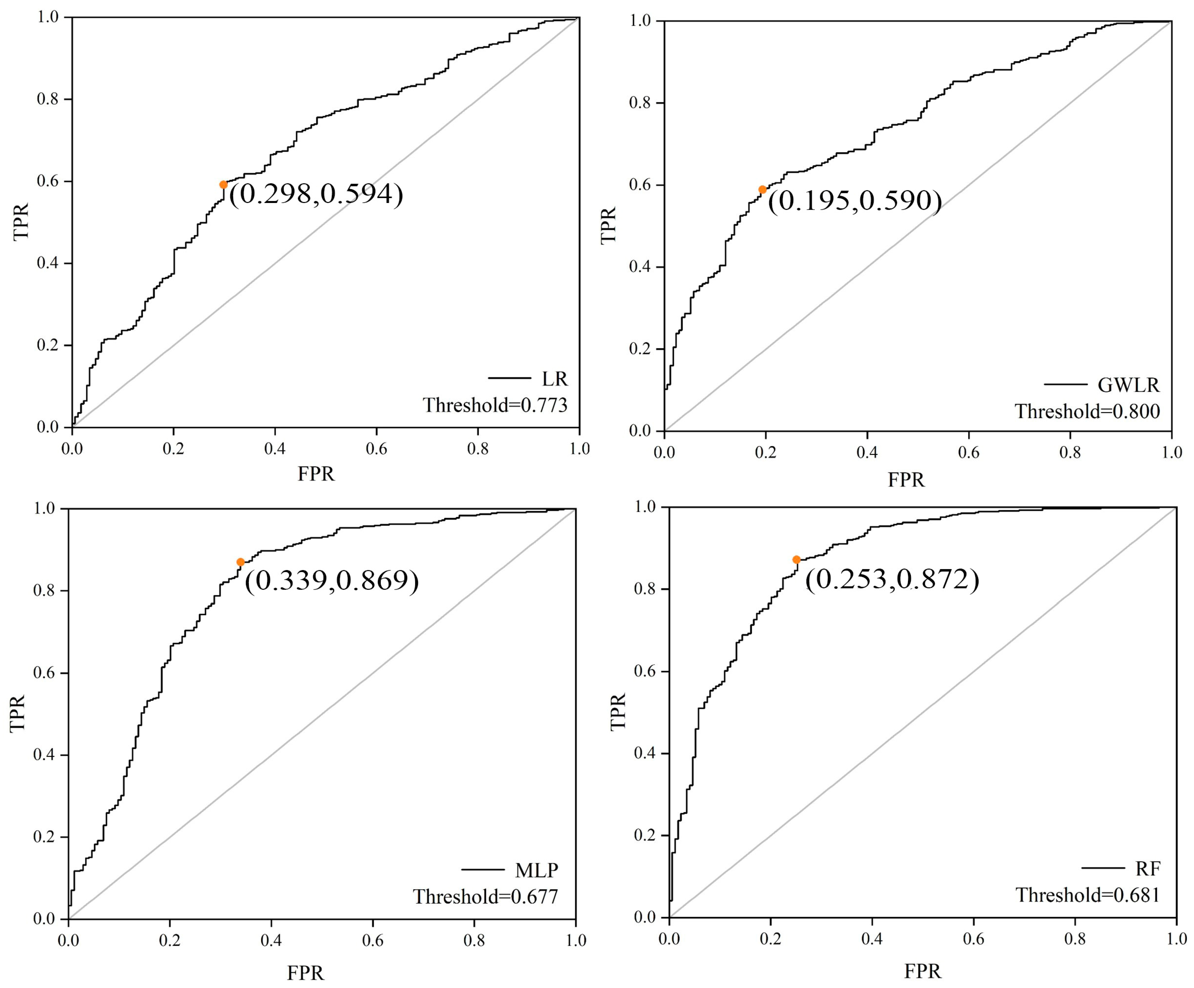
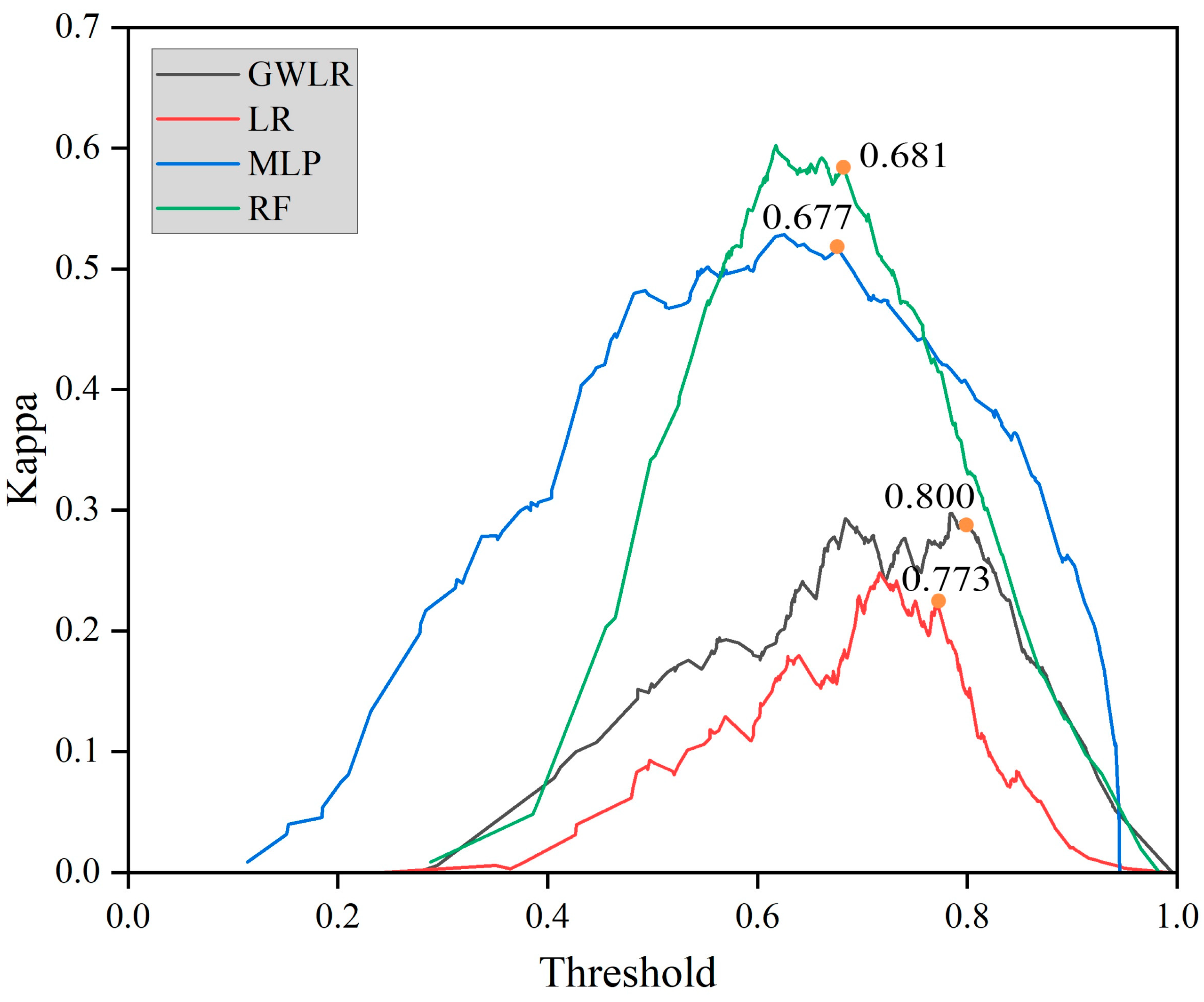
2.3. Model Evaluation
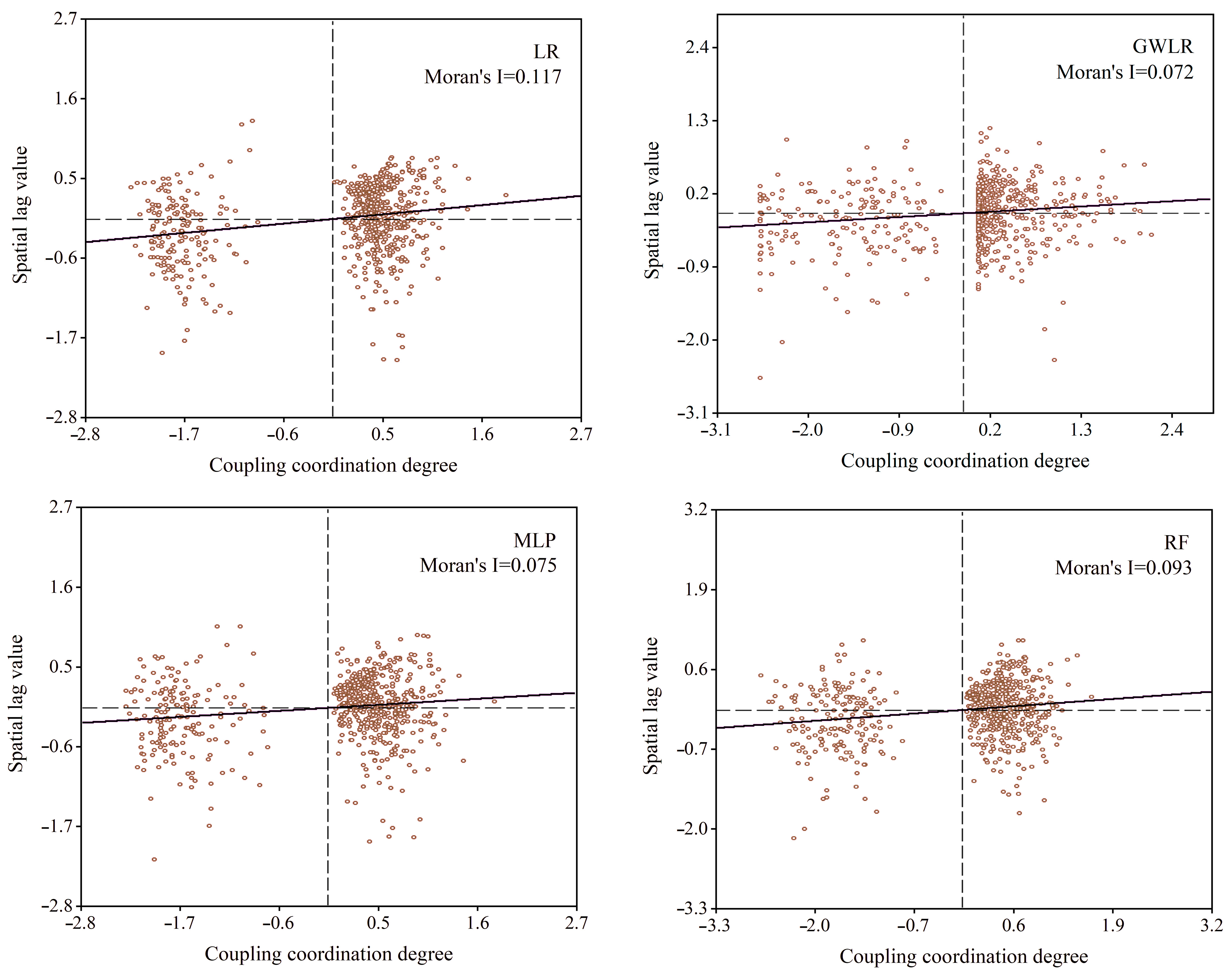
2.4. Spatial Autocorrelation Test of Model Residuals
3. Results
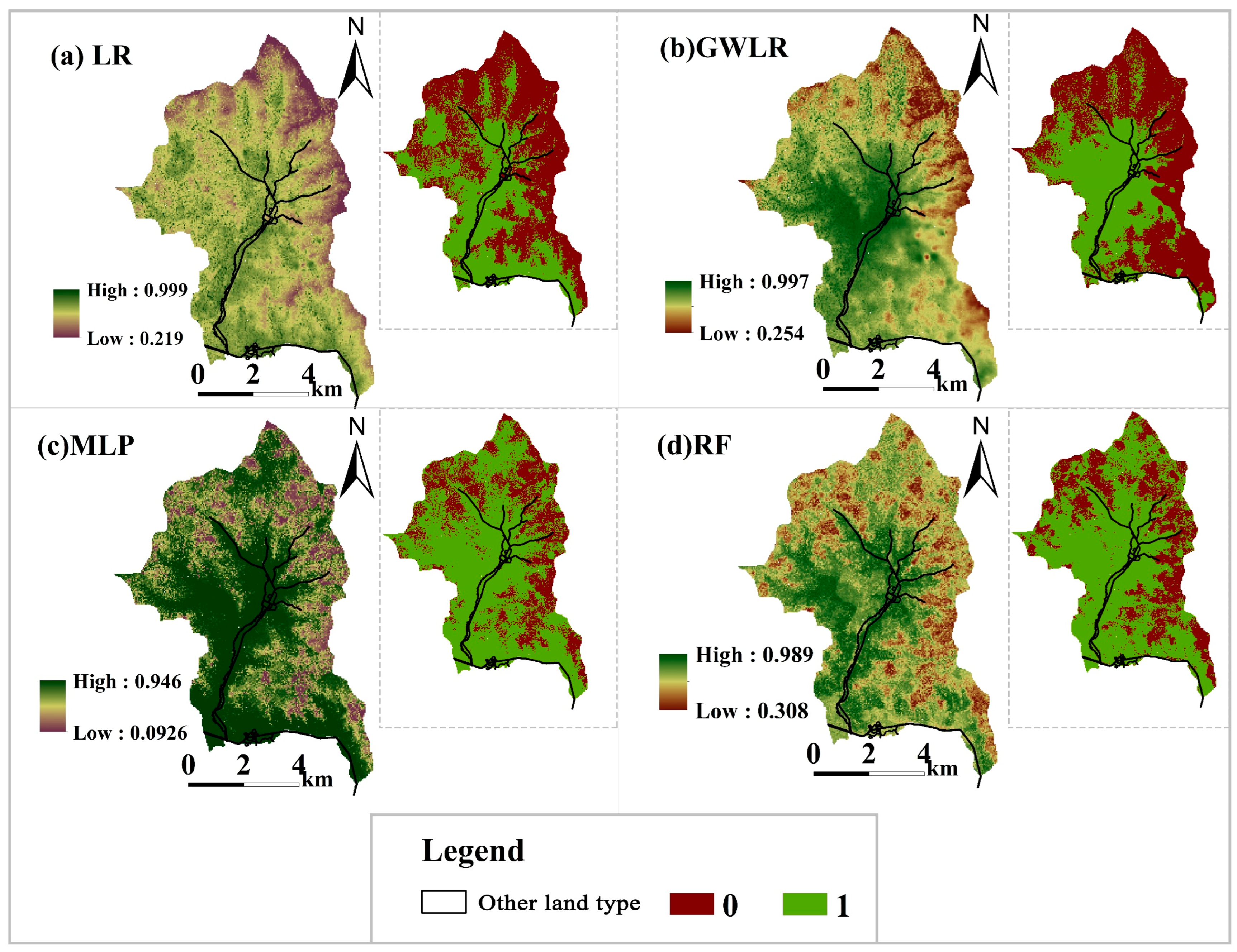
3.1. Fitting Results of Models
3.2. Model Accuracy Evaluation
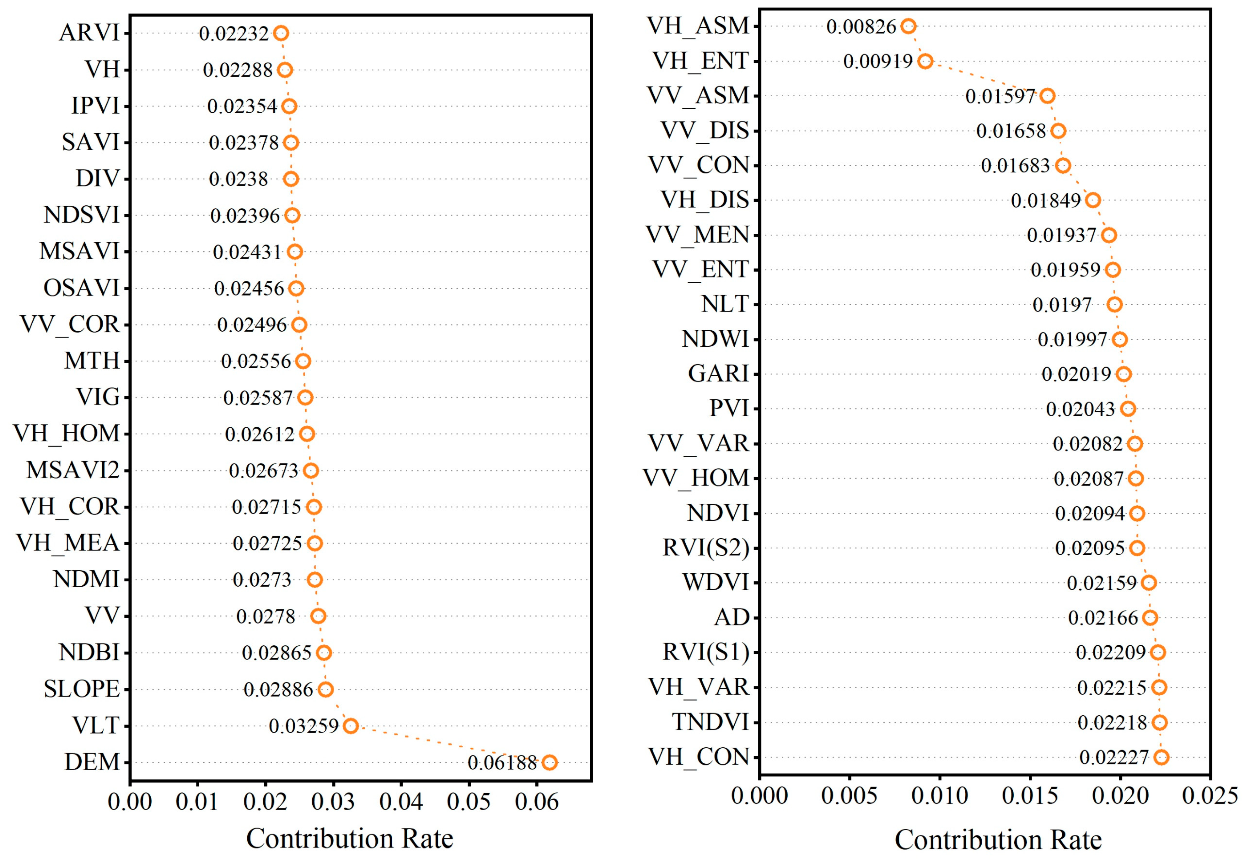
3.3. RF Model Importance Ranking
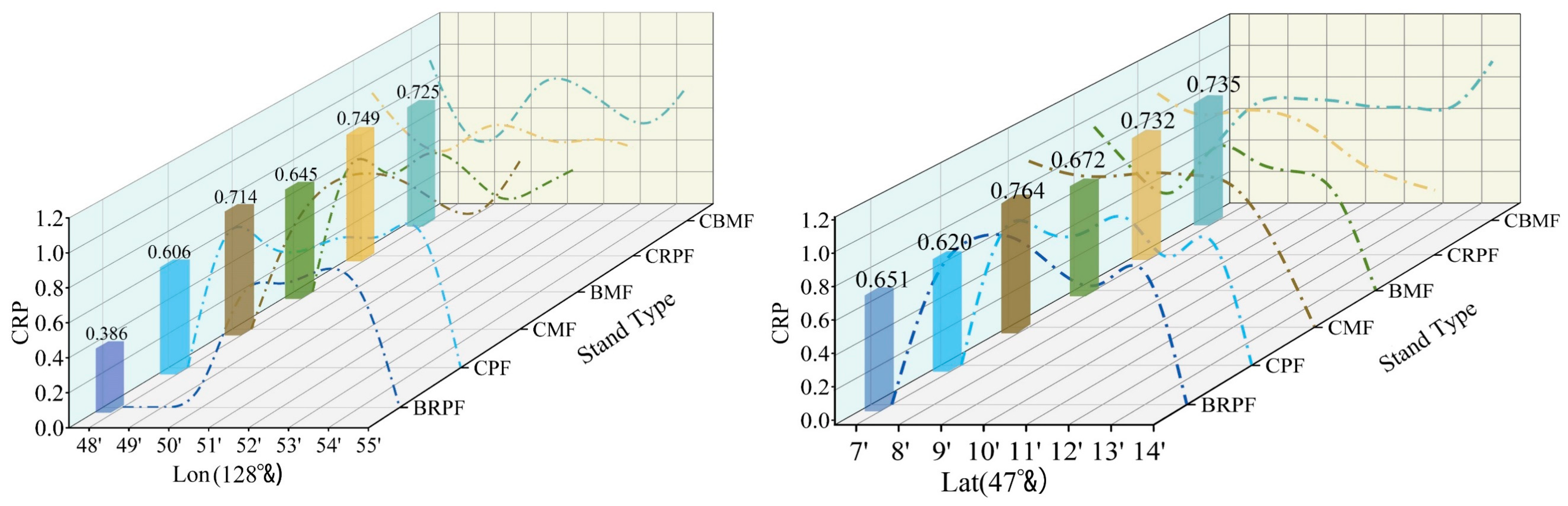
3.4. Analysis of Understory Regeneration Law
4. Discussion
4.1. Model Variable Selection
4.2. Selected Predictor Variables and Their Ecological Implications
4.3. Model Comparison
4.4. Advantages of Optimal Threshold Segmentation
5. Conclusions
- The RF model achieved the highest value of accuracy evaluation. However, the RF model has the disadvantage of neglecting the spatial autocorrelation among neighboring samples. The GWLR model, constructed by LR regression, effectively accounts for the spatial autocorrelation among neighboring samples.
- The distribution of CRP along the latitude and longitude lines exhibited spatial heterogeneity.
- The DEM variable was the most significant factor influencing CRP.
- Coniferous sapling regeneration mainly occurred in low-latitude and low-longitude regions, and most pixels in the high-latitude and high-longitude regions of the study had a CRP value of 0, indicating that no coniferous sapling regeneration occurred.
Author Contributions
Funding
Data Availability Statement
Conflicts of Interest
References
- Haq, S.M.; Amjad, M.S.; Waheed, M.; Bussmann, R.W.; Proćków, J. The floristic quality assessment index as ecological health indicator for forest vegetation: A case study from Zabarwan Mountain Range, Himalayas. Ecol. Indic. 2022, 145, 109670. [Google Scholar] [CrossRef]
- Constant, N.L.; Taylor, P.J. Restoring the forest revives our culture: Ecosystem services and values for ecological restoration across the rural-urban nexus in South Africa. For. Policy Econ. 2020, 118, 102222. [Google Scholar] [CrossRef]
- de Pater, C.; Verschuuren, B.; Elands, B.; van Hal, I.; Turnhout, E. Spiritual values in forest management plans in British Columbia and the Netherlands. For. Policy Econ. 2023, 151, 102955. [Google Scholar] [CrossRef]
- Taye, F.A.; Folkersen, M.V.; Fleming, C.M.; Buckwell, A.; Mackey, B.; Diwakar, K.C.; Le, D.; Hasan, S.; Ange, C.S. The economic values of global forest ecosystem services: A meta-analysis. Ecol. Econ. 2021, 189, 107145. [Google Scholar] [CrossRef]
- Hammond, M.E.; Pokorný, R.; Okae-Anti, D.; Gyedu, A.; Obeng, I.O. The composition and diversity of natural regeneration of tree species in gaps under different intensities of forest disturbance. J. For. Res. 2021, 32, 1843–1853. [Google Scholar] [CrossRef]
- Aide, T.M.; Zimmerman, J.K.; Pascarella, J.B.; Rivera, L.; Ecology, H.M.V.J.R. Forest Regeneration in a Chronosequence of Tropical Abandoned Pastures: Implications for Restoration Ecology. Restor. Ecol. 2000, 8, 328–338. [Google Scholar] [CrossRef]
- Maciel-Nájera, J.F.; Hernández-Velasco, J.; González-Elizondo, M.S.; Hernández-Díaz, J.C.; López-Sánchez, C.A.; Antúnez, P.; Bailón-Soto, C.E.; Wehenkel, C. Unexpected spatial patterns of natural regeneration in typical uneven-aged mixed pine-oak forests in the Sierra Madre Occidental, Mexico. Glob. Ecol. Conserv. 2020, 23, e01074. [Google Scholar] [CrossRef]
- Boag, A.E.; Ducey, M.J.; Palace, M.W.; Hartter, J. Topography and fire legacies drive variable post-fire juvenile conifer regeneration in eastern Oregon, USA. For. Ecol. Manag. 2020, 474, 118312. [Google Scholar] [CrossRef]
- Liu, F.; Tan, C.; Yang, Z.; Li, J.; Xiao, H.; Tong, Y. Regeneration and growth of tree seedlings and saplings in created gaps of different sizes in a subtropical secondary forest in southern China. For. Ecol. Manag. 2022, 511, 120143. [Google Scholar] [CrossRef]
- Chen, H.H.; Zhu, X.; Zhu, G.Y.; Liu, F.H. Effects of stand structure on understory biomass of the Quercus spp secondary forests in Hunan Province, China. J. Appl. Ecol. 2020, 31, 349–356. [Google Scholar]
- Hu, T.; Sun, Y.; Jia, W.; Li, D.; Zou, M.; Zhang, M. Study on the Estimation of Forest Volume Based on Multi-Source Data. Sensors 2021, 21, 7796. [Google Scholar] [CrossRef] [PubMed]
- Lee, L.X.; Whitby, T.G.; Munger, J.W.; Stonebrook, S.J.; Friedl, M.A. Remote sensing of seasonal variation of LAI and fAPAR in a deciduous broadleaf forest. Agric. For. Meteorol. 2023, 333, 109389. [Google Scholar] [CrossRef]
- Iglseder, A.; Immitzer, M.; Dostálová, A.; Kasper, A.; Pfeifer, N.; Bauerhansl, C.; Schöttl, S.; Hollaus, M. The potential of combining satellite and airborne remote sensing data for habitat classification and monitoring in forest landscapes. Int. J. Appl. Earth Obs. Geoinf. 2023, 117, 103131. [Google Scholar] [CrossRef]
- Puliti, S.; Breidenbach, J.; Schumacher, J.; Hauglin, M.; Klingenberg, T.F.; Astrup, R. Above-ground biomass change estimation using national forest inventory data with Sentinel-2 and Landsat. Remote Sens. Environ. 2021, 265, 112644. [Google Scholar] [CrossRef]
- Persson, H.J.; Ekström, M.; Ståhl, G. Quantify and account for field reference errors in forest remote sensing studies. Remote Sens. Environ. 2022, 283, 113302. [Google Scholar] [CrossRef]
- Tariq, S.; Nawaz, H.; Mehmood, U.; ul Haq, Z.; Pata, U.K.; Murshed, M. Remote sensing of air pollution due to forest fires and dust storm over Balochistan (Pakistan). Atmos. Pollut. Res. 2023, 14, 101674. [Google Scholar] [CrossRef]
- Stahl, A.T.; Andrus, R.; Hicke, J.A.; Hudak, A.T.; Bright, B.C.; Meddens, A.J.H. Automated attribution of forest disturbance types from remote sensing data: A synthesis. Remote Sens. Environ. 2023, 285, 113416. [Google Scholar] [CrossRef]
- Kumar, R.; Nandy, S.; Agarwal, R.; Kushwaha, S.P.S. Forest cover dynamics analysis and prediction modeling using logistic regression model. Ecol. Indic. 2014, 45, 444–455. [Google Scholar] [CrossRef]
- Basu, T.; Das, A.; Pereira, P. Exploring the drivers of urban expansion in a medium-class urban agglomeration in India using the remote sensing techniques and geographically weighted models. Geogr. Sustain. 2023, 4, 150–160. [Google Scholar] [CrossRef]
- Fotheringham, A.S.; Charlton, M.E.; Brunsdon, C. Geographically Weighted Regression: A Natural Evolution of the Expansion Method for Spatial Data Analysis. Environ. Plan. A Econ. Space 2016, 30, 1905–1927. [Google Scholar] [CrossRef]
- Sun, Y.; Ao, Z.; Jia, W.; Chen, Y.; Xu, K. A geographically weighted deep neural network model for research on the spatial distribution of the down dead wood volume in Liangshui National Nature Reserve (China). Iforest-Biogeosci. For. 2021, 14, 353–361. [Google Scholar] [CrossRef]
- Brunsdon, C.; Fotheringham, A.S.; Charlton, M.E. Geographically Weighted Regression: A Method for Exploring Spatial Nonstationarity. Geogr. Anal. 2010, 28, 281–298. [Google Scholar] [CrossRef]
- Cui, Y.; Pan, C.; Liu, C.; Luo, M.; Guo, Y. Spatiotemporal variation and tendency analysis on rainfall erosivity in the Loess Plateau of China. Hydrol. Res. 2020, 51, 1048–1062. [Google Scholar] [CrossRef]
- Liu, D.; Clarke, K.C.; Chen, N. Integrating spatial nonstationarity into SLEUTH for urban growth modeling: A case study in the Wuhan metropolitan area. Comput. Environ. Urban Syst. 2020, 84, 101545. [Google Scholar] [CrossRef]
- Ali, M.R.; Nipu, S.M.A.; Khan, S.A. A decision support system for classifying supplier selection criteria using machine learning and random forest approach. Decis. Anal. J. 2023, 7, 100238. [Google Scholar] [CrossRef]
- Ghosh, A.; Dey, P. Flood Severity assessment of the coastal tract situated between Muriganga and Saptamukhi estuaries of Sundarban delta of India using Frequency Ratio (FR), Fuzzy Logic (FL), Logistic Regression (LR) and Random Forest (RF) models. Reg. Stud. Mar. Sci. 2021, 42, 101624. [Google Scholar] [CrossRef]
- Billah, M.; Islam, A.K.M.S.; Mamoon, W.B.; Rahman, M.R. Random forest classifications for landuse mapping to assess rapid flood damage using Sentinel-1 and Sentinel-2 data. Remote Sens. Appl. Soc. Environ. 2023, 30, 100947. [Google Scholar] [CrossRef]
- Zermane, A.; Mohd Tohir, M.Z.; Zermane, H.; Baharudin, M.R.; Mohamed Yusoff, H. Predicting fatal fall from heights accidents using random forest classification machine learning model. Saf. Sci. 2023, 159, 106023. [Google Scholar] [CrossRef]
- Karimi, B.; Hashemi, S.H.; Aghighi, H. Development of the best retrieval models of non-optically active parameters for an artificial shallow lake by random forest algorithm. Remote Sens. Appl. Soc. Environ. 2023, 29, 100926. [Google Scholar] [CrossRef]
- Ghazvini, M.; Varedi-Koulaei, S.M.; Ahmadi, M.H.; Kim, M. Optimization of MLP neural network for modeling flow boiling performance of Al2O3/water nanofluids in a horizontal tube. Eng. Anal. Bound. Elem. 2022, 145, 363–395. [Google Scholar] [CrossRef]
- Martínez-Comesaña, M.; Ogando-Martínez, A.; Troncoso-Pastoriza, F.; López-Gómez, J.; Febrero-Garrido, L.; Granada-Álvarez, E. Use of optimised MLP neural networks for spatiotemporal estimation of indoor environmental conditions of existing buildings. Build. Environ. 2021, 205, 108243. [Google Scholar] [CrossRef]
- Wang, F.; Sun, Y.; Jia, W.; Zhu, W.; Li, D.; Zhang, X.; Tang, Y.; Guo, H. Development of Estimation Models for Individual Tree Aboveground Biomass Based on TLS-Derived Parameters. Forests 2023, 14, 351. [Google Scholar] [CrossRef]
- Li, H.; Zhang, G.; Zhong, Q.; Xing, L.; Du, H. Prediction of Urban Forest Aboveground Carbon Using Machine Learning Based on Landsat 8 and Sentinel-2: A Case Study of Shanghai, China. Remote Sens. 2023, 15, 284. [Google Scholar] [CrossRef]
- Meng, X.; Li, F. Forest Mensuration, 3rd ed.; China Forestry Publishing House: Beijing, China, 2006; pp. 28, 59, 61, 63, 67. [Google Scholar]
- Vanderhoof, M.K.; Alexander, L.; Christensen, J.; Solvik, K.; Nieuwlandt, P.; Sagehorn, M. High-frequency time series comparison of Sentinel-1 and Sentinel-2 satellites for mapping open and vegetated water across the United States (2017–2021). Remote Sens. Environ. 2023, 288, 113498. [Google Scholar] [CrossRef]
- Liu, X.; Frey, J.; Munteanu, C.; Still, N.; Koch, B. Mapping tree species diversity in temperate montane forests using Sentinel-1 and Sentinel-2 imagery and topography data. Remote Sens. Environ. 2023, 292, 113576. [Google Scholar] [CrossRef]
- Sandhini Putri, A.F.; Widyatmanti, W.; Umarhadi, D.A. Sentinel-1 and Sentinel-2 data fusion to distinguish building damage level of the 2018 Lombok Earthquake. Remote Sens. Appl. Soc. Environ. 2022, 26, 100724. [Google Scholar] [CrossRef]
- Collins, M.J.; Wiebe, J.; Clausi, D.A. The effect of speckle filtering on scale-dependent texture estimation of a forested scene. IEEE Trans. Geosci. Remote Sens. 2000, 38, 1160–1170. [Google Scholar] [CrossRef]
- Prasad, T.S.; Gupta, R.K. Texture based classification of multidate SAR images—A case study. Geocarto Int. 1998, 13, 53–62. [Google Scholar] [CrossRef]
- Desloires, J.; Ienco, D.; Botrel, A. Out-of-year corn yield prediction at field-scale using Sentinel-2 satellite imagery and machine learning methods. Comput. Electron. Agric. 2023, 209, 107807. [Google Scholar] [CrossRef]
- Eskandari, S.; Ali Mahmoudi Sarab, S. Mapping land cover and forest density in Zagros forests of Khuzestan province in Iran: A study based on Sentinel-2, Google Earth and field data. Ecol. Inform. 2022, 70, 101727. [Google Scholar] [CrossRef]
- Yang, X.; Qiu, S.; Zhu, Z.; Rittenhouse, C.; Riordan, D.; Cullerton, M. Mapping understory plant communities in deciduous forests from Sentinel-2 time series. Remote Sens. Environ. 2023, 293, 113601. [Google Scholar] [CrossRef]
- Baret, F.; Guyot, G. Potentials and limits of vegetation indices for LAI and APAR assessment. Remote Sens. Environ. 1991, 35, 161–173. [Google Scholar] [CrossRef]
- Crippen, R.E. Calculating the vegetation index faster. Remote Sens. Environ. 1990, 34, 71–73. [Google Scholar] [CrossRef]
- Li, W.; Li, C.; Jiang, L. Learning from crowds with robust logistic regression. Inf. Sci. 2023, 639, 119010. [Google Scholar] [CrossRef]
- Karabadji, N.E.I.; Amara Korba, A.; Assi, A.; Seridi, H.; Aridhi, S.; Dhifli, W. Accuracy and diversity-aware multi-objective approach for random forest construction. Expert Syst. Appl. 2023, 225, 120138. [Google Scholar] [CrossRef]
- Dong, Y.-H.; Peng, F.-L.; Li, H.; Men, Y.-Q. Spatial autocorrelation and spatial heterogeneity of underground parking space development in Chinese megacities based on multisource open data. Appl. Geogr. 2023, 153, 102897. [Google Scholar] [CrossRef]
- Hoyos, N.; Escobar, J.; Restrepo, J.C.; Arango, A.M.; Ortiz, J.C. Impact of the 2010–2011 La Niña phenomenon in Colombia, South America: The human toll of an extreme weather event. Appl. Geogr. 2013, 39, 16–25. [Google Scholar] [CrossRef]
- Young, S.G.; Jensen, R.R. Statistical and visual analysis of human West Nile virus infection in the United States, 1999–2008. Appl. Geogr. 2012, 34, 425–431. [Google Scholar] [CrossRef]
- Moran, P.A.P. The Interpretation of Statistical Maps. J. R. Stat. Soc. Ser. B Methodol. 1948, 10, 243–251. [Google Scholar] [CrossRef]
- Yang, H.; Pan, C.; Wu, Y.; Qing, S.; Wang, Z.; Wang, D. Response of understory plant species richness and tree regeneration to thinning in Pinus tabuliformis plantations in northern China. For. Ecosyst. 2023, 10, 100105. [Google Scholar] [CrossRef]
- Erdozain, M.; Bonet, J.A.; Martínez de Aragón, J.; de-Miguel, S. Forest thinning and climate interactions driving early-stage regeneration dynamics of maritime pine in Mediterranean areas. For. Ecol. Manag. 2023, 539, 121036. [Google Scholar] [CrossRef]
- Bruun, H.H.; Moen, J.; Virtanen, R.; Grytnes, J.A.; Oksanen, L.; Angerbjörn, A. Effects of altitude and topography on species richness of vascular plants, bryophytes and lichens in alpine communities. J. Veg. Sci. 2010, 17, 37–46. [Google Scholar] [CrossRef]
- Qin, Y.; He, X.; Lei, X.; Feng, L.; Zhou, Z.; Lu, J. Tree size inequality and competition effects on nonlinear mixed effects crown width model for natural spruce-fir-broadleaf mixed forest in northeast China. For. Ecol. Manag. 2022, 518, 120291. [Google Scholar] [CrossRef]
- Birungi, V.; Dejene, S.W.; Mbogga, M.S.; Dumas-Johansen, M. Carbon stock of Agoro Agu Central Forest reserve, in Lamwo district, Northern Uganda. Heliyon 2023, 9, e14252. [Google Scholar] [CrossRef] [PubMed]
- Basyuni, M.; Wirasatriya, A.; Iryanthony, S.B.; Amelia, R.; Slamet, B.; Sulistiyono, N.; Pribadi, R.; Sumarga, E.; Eddy, S.; Al Mustaniroh, S.S.; et al. Aboveground biomass and carbon stock estimation using UAV photogrammetry in Indonesian mangroves and other competing land uses. Ecol. Inform. 2023, 77, 102227. [Google Scholar] [CrossRef]
- Salete Capellesso, E.; Cequinel, A.; Marques, R.; Luisa Sausen, T.; Bayer, C.; Marques, M.C.M. Co-benefits in biodiversity conservation and carbon stock during forest regeneration in a preserved tropical landscape. For. Ecol. Manag. 2021, 492, 119222. [Google Scholar] [CrossRef]
- Hart, E.; Sim, K.; Kamimura, K.; Meredieu, C.; Guyon, D.; Gardiner, B. Use of machine learning techniques to model wind damage to forests. Agric. For. Meteorol. 2019, 265, 16–29. [Google Scholar] [CrossRef]
- Dobrini, D.; Gaparovi, M.; Medak, D.J.R.S. Sentinel-1 and 2 Time-Series for Vegetation Mapping Using Random Forest Classification: A Case Study of Northern Croatia. Remote Sens. 2021, 13, 2321. [Google Scholar] [CrossRef]

| Tree Species Type | Volume Formula |
|---|---|
| Korean pine | 0.00010339412 × (−0.005162178 + 0.975389083 × DBH)^ (2.5550714) |
| Spruce | 0.000097559294 × (−0.023269474 + 0.979033877 × DBH)^ (2.6082001) |
| Fir | 0.00012553802 × (−0.14050637 + 0.976669654 × DBH)^ (2.5301655) |
| Camphor pine | 0.0002380777 × (−0.1661345 + 0.983825482 × DBH)^ (2.3888099) |
| Larch | 0.00005016824 × (−0.1661345 + 0.983825482 × DBH)^1.7582894 × (1.6504613 + 0.78031609 × (−0.1661345 + 0.983825482 × DBH) −0.0076188678 × (−0.1661345 + 0.983825482×DBH)^2)^ (1.1496653) |
| Pinus densiflora | 0.00016773252 × (0.1539054215 + 0.981705489 × DBH)^ (2.2855543) |
| Fraxinus mandshurica Rupr. | 0.000041960698 × (−0.0283700973 + 0.969811198 ×DBH)^ (1.9094595) × (5.6382753 + 0.64085 × (−0.0283700973 + 0.969811198 × DBH) −0.0056371339 × (−0.0283700973 + 0.969811198 ×DBH)^2)^ (1.0413892) |
| Juglans mandshurica | 0.000041960698 × (−0.1068104174 + 0.975403018×DBH)^ (1.9094595) × (6.5706028 + 0.51071923 × (−0.1068104174 + 0.975403018 × DBH) −0.0034904923 × (−0.1068104174 + 0.975403018 × DBH)^2)^ (1.0413892) |
| Phellodendron | 0.00018200258 × (−0.2516967596 + 0.972900665 × DBH)^ (2.3187749) |
| Linden tree | 0.000041960698 × (0.2250730369 + 0.964592149 × DBH)^ (1.9094595) × (5.2592429 + 0.5670384 × (0.2250730369 + 0.964592149 × DBH) −0.0038177352 × (0.2250730369 + 0.964592149 × DBH)^2)^ (1.0413892) |
| Oak | 0.00025462482 × (0.1751205585 + 0.986711062 × DBH)^ (2.1935242) |
| Elm | 0.00013344177 × (−0.120162996 + 0.971592141 × DBH)^ (2.4489629) |
| Maple birch | 0.000041960698 × (0.040314124 + 0.957532468 × DBH)^ (1.9094595) × (7.0086039 + 0.6791334 × (0.040314124 + 0.957532468 × DBH) −0.0063965703 × (0.040314124 + 0.957532468 × DBH)^ (2))^ (1.0413892) |
| Black birch | 0.000052786451 × (−0.4899312906 + 0.995171441 × DBH)^ (1.7947313) × (6.2804214 + 0.46824315 × (−0.4899312906 + 0.995171441 × DBH) −0.0046635886 × (−0.4899312906 + 0.995171441 × DBH)^2)^ (1.0712623) |
| Sapling Height | Min | SD | Mean | Max | |
|---|---|---|---|---|---|
| <130 cm | Basal diameter (BD, cm) | 0.5 | 0.645 | 1.476 | 3.963 |
| Diameter breast height (DBH, cm) | – | – | – | – | |
| Age | 5 | 2.796 | 9.411 | 16 | |
| Height (H, cm) | 5 | 28.204 | 84.263 | 129 | |
| ≥130 cm | Basal diameter (BD, cm) | 0.7 | 1.522 | 3.635 | 7.512 |
| Diameter breast height (DBH, cm) | 0.1 | 1.080 | 0.532 | 2.360 | |
| Age | 10 | 2.274 | 14.115 | 17 | |
| Height (H, cm) | 132 | 97.831 | 286.825 | 610 |
| Variable | Min | SD | Mean | Max |
|---|---|---|---|---|
| CRP | 0 | 0.431 | 0.755 | 1 |
| NLT (n/ha) | 200 | 356.158 | 805.590 | 3083.333 |
| AD (cm) | 9.85 | 4.210 | 19.653 | 40.85 |
| VLT (m3/ha) | 31.081 | 59.34893 | 193.807 | 402.243 |
| MTH (m) | 8.8 | 4.899 | 20.913 | 39.117 |
| Stand Type | Number of Sample Plots | Percentage |
|---|---|---|
| Broadleaf Mixed Forest (BMF) | 106 | 15.9% |
| Broadleaf Relatively Pure Forest (BRPF) | 20 | 3.01% |
| Coniferous Broadleaved Mixed Forest (CBMF) | 244 | 36.7% |
| Coniferous Pure Forest (CPF) | 26 | 3.91% |
| Coniferous Mixed Forest (CMF) | 152 | 22.9% |
| Coniferous Relatively Pure Forest (CRPF) | 117 | 17.6% |
| 47°& | 7′ | 8′ | 9′ | 10′ | 11′ | 12′ | 13′ | 14′ | CRP Mean | |
|---|---|---|---|---|---|---|---|---|---|---|
| Stand Type | ||||||||||
| Broadleaf Mixed Forest (BMF) | 1 | 0.724 | 0.478 | 1 | 0.75 | 0.727 | 0.7 | 0 | 0.672 | |
| Broadleaf Relatively Pure Forest (BRPF) | 0 | 0.833 | 1 | 1 | 0.75 | 0.625 | 1 | 0 | 0.651 | |
| Coniferous Broadleaved Mixed Forest (CBMF) | 0.5 | 0.794 | 0.759 | 0.759 | 0.696 | 0.725 | 0.643 | 1 | 0.735 | |
| Coniferous Pure Forest (CPF) | 0 | 1 | 0.75 | 0.75 | 1 | 0.462 | 1 | 0 | 0.620 | |
| Coniferous Mixed Forest (CMF) | 1 | 0.909 | 0.9 | 0.941 | 0.911 | 0.909 | 0.542 | 0 | 0.764 | |
| Coniferous Relatively Pure Forest (CRPF) | 1 | 0.833 | 0.905 | 0.895 | 0.794 | 0.565 | 0.467 | 0.4 | 0.732 | |
| 128°& | 48′ | 49′ | 50′ | 51′ | 52′ | 53′ | 54′ | 55′ | CRP Mean | |
|---|---|---|---|---|---|---|---|---|---|---|
| Stand Type | ||||||||||
| Broadleaf Mixed Forest (BMF) | 0 | 1 | 0.6 | 0.905 | 0.769 | 0.5 | 0.636 | 0.750 | 0.645 | |
| Broadleaf Relatively Pure Forest (BRPF) | 0 | 0 | 0 | 0.8 | 0.667 | 0.818 | 0.800 | 0 | 0.386 | |
| Coniferous Broadleaved Mixed Forest (CBMF) | 1 | 0.444 | 0.5 | 0.929 | 0.868 | 0.686 | 0.541 | 0.833 | 0.725 | |
| Coniferous Pure Forest (CPF) | 0 | 1 | 0.667 | 0.667 | 0.8 | 0.714 | 1 | 0 | 0.606 | |
| Coniferous Mixed Forest (CMF) | 0 | 0.625 | 0.889 | 0.944 | 0.897 | 0.72 | 0.636 | 1 | 0.714 | |
| Coniferous Relatively Pure Forest (CRPF) | 1 | 0.714 | 0.583 | 0.833 | 0.786 | 0.667 | 0.739 | 0.667 | 0.749 | |
| Variable | Estimate | Standard Error | p Value | Exp—(Est) |
|---|---|---|---|---|
| Intercept | 1.219 | 0.094 | 0.000 | 3.385 |
| AD (cm) | 0.313 | 0.121 | 0.010 | 1.367 |
| VLT (m3/ha) | −0.180 | 0.099 | 0.030 | 0.835 |
| VV_VAR | 0.173 | 0.106 | 0.031 | 1.189 |
| VH_CON | 0.311 | 0.132 | 0.018 | 1.365 |
| GARI | 0.073 | 0.099 | 0.046 | 1.076 |
| DEM (m) | −0.557 | 0.107 | 0.000 | 0.573 |
| Variable | Min | Lower Quartile | Mean | Median | Upper Quartile | Max |
|---|---|---|---|---|---|---|
| Intercept | 0.884 | 1.162 | 1.271 | 1.262 | 1.386 | 1.709 |
| AD (cm) | 0.032 | 0.207 | 0.347 | 0.287 | 0.384 | 0.999 |
| VLT (m3/ha) | −0.426 | −0.308 | −0.203 | −0.250 | −0.103 | 0.152 |
| VV_VAR | −0.011 | 0.075 | −0.182 | 0.135 | 0.257 | 0.623 |
| VH_CON | −0.104 | 0.029 | 0.232 | 0.209 | 0.423 | 0.615 |
| GARI | −0.261 | −0.093 | 0.050 | 0.055 | 0.174 | 0.466 |
| DEM (m) | −2.506 | −0.926 | −0.819 | −0.659 | −0.545 | −0.381 |
| Model | AUC | Threshold | KAPPA | RMSE | MAE |
|---|---|---|---|---|---|
| LR | 0.684 | 0.772 | 0.225 | 0.416 | 0.346 |
| GWLR | 0.751 | 0.811 | 0.277 | 0.400 | 0.315 |
| MLP | 0.843 | 0.677 | 0.463 | 0.350 | 0.260 |
| RF | 0.867 | 0.633 | 0.561 | 0.332 | 0.240 |
Disclaimer/Publisher’s Note: The statements, opinions and data contained in all publications are solely those of the individual author(s) and contributor(s) and not of MDPI and/or the editor(s). MDPI and/or the editor(s) disclaim responsibility for any injury to people or property resulting from any ideas, methods, instructions or products referred to in the content. |
© 2023 by the authors. Licensee MDPI, Basel, Switzerland. This article is an open access article distributed under the terms and conditions of the Creative Commons Attribution (CC BY) license (https://creativecommons.org/licenses/by/4.0/).
Share and Cite
Zhao, H.; Sun, Y.; Jia, W.; Wang, F.; Zhao, Z.; Wu, S. Study on the Regeneration Probability of Understory Coniferous Saplings in the Liangshui Nature Reserve Based on Four Modeling Techniques. Remote Sens. 2023, 15, 4869. https://doi.org/10.3390/rs15194869
Zhao H, Sun Y, Jia W, Wang F, Zhao Z, Wu S. Study on the Regeneration Probability of Understory Coniferous Saplings in the Liangshui Nature Reserve Based on Four Modeling Techniques. Remote Sensing. 2023; 15(19):4869. https://doi.org/10.3390/rs15194869
Chicago/Turabian StyleZhao, Haiping, Yuman Sun, Weiwei Jia, Fan Wang, Zipeng Zhao, and Simin Wu. 2023. "Study on the Regeneration Probability of Understory Coniferous Saplings in the Liangshui Nature Reserve Based on Four Modeling Techniques" Remote Sensing 15, no. 19: 4869. https://doi.org/10.3390/rs15194869
APA StyleZhao, H., Sun, Y., Jia, W., Wang, F., Zhao, Z., & Wu, S. (2023). Study on the Regeneration Probability of Understory Coniferous Saplings in the Liangshui Nature Reserve Based on Four Modeling Techniques. Remote Sensing, 15(19), 4869. https://doi.org/10.3390/rs15194869