Article

Ecosystem Evapotranspiration Partitioning and Its Spatial–Temporal Variation Based on Eddy Covariance Observation and Machine Learning Method

1
Remote Sensing Information and Digital Earth Center, College of Computer Science and Technology, Qingdao University, Qingdao 266071, China
2
Key Laboratory of Digital Earth Science, Aerospace Information Research Institute, Chinese Academy of Sciences, Beijing 100094, China
*
Author to whom correspondence should be addressed.
Remote Sens. 2023, 15(19), 4831; https://doi.org/10.3390/rs15194831
Submission received: 14 August 2023 / Revised: 17 September 2023 / Accepted: 29 September 2023 / Published: 5 October 2023
(This article belongs to the Section Remote Sensing for Geospatial Science)

Abstract

:
Partitioning evapotranspiration (ET) into vegetation transpiration (T) and soil evaporation (E) is challenging, but it is key to improving the understanding of plant water use and changes in terrestrial ecosystems. Considering that the transpiration of vegetation at night is minimal and can be negligible, we established a machine learning model (i.e., extreme gradient boosting algorithm (XGBoost)) for soil evaporation estimation based on night-time evapotranspiration observation data from eddy covariance towers, remote sensing data, and meteorological reanalysis data. Daytime T was consequently calculated as the difference between the total evapotranspiration and predicted daytime soil evaporation. The soil evaporation estimation model was validated based on the remaining night-time ET data (i.e., model test dataset), the non-growing season ET data of the natural ecosystem, and ET data during the fallow periods of croplands. The validation results showed that XGBoost had a better performance in E estimation, with the average overall accuracy of NSE 0.657, R 0.806, and RMSE 11.344 W/m2. The average annual T/ET of the examined ten ecosystems was 0.50 ± 0.08, with the highest value in deciduous broadleaf forests (0.68 ± 0.11), followed by mixed forests (0.61 ± 0.04), and the lowest in croplands (0.40 ± 0.08). We further examined the impact of the leaf area index (LAI) and vapor pressure deficit (VPD) on the variation in T/ET. Overall, at the interannual scale, LAI contributed 28% to the T/ET variation, while VPD had a small (5%) influence. On a seasonal scale, LAI also exerted a stronger impact (1~90%) on T/ET compared to VPD (1~77%). Our study suggests that the XGBoost machine learning model has good performance in ET partitioning, and this method is mainly data-driven without prior knowledge, which may provide a simple and valuable method in global ET partitioning and T/ET estimation.

1. Introduction

Evapotranspiration (ET), consisting of soil evaporation (E) and plant transpiration (T), is a complex eco-hydrological process of terrestrial ecosystems. It plays a vital role in the global carbon–water exchange and land–atmosphere interactions [1]. As a key component of ET, transpiration accounts for the majority of ET with range of 20–95% at the global scale [2,3]. Transpiration reflects vegetation water use directly, and accurate estimation of T is of great significance for understanding the global water cycle and the coupling relationship between carbon and water cycles [4]. However, it is highly challenging to accurately partition ET into T and E or directly estimate T, especially in the ecosystem scale.
At the ecosystem scale, there are no satisfied techniques to directly and quickly observe ecosystem transpiration. Traditional measurement techniques, such as sap flow sensors [5] and stable isotopes [6,7], which can determine E and T components by direct measurements, are considered reliable methods for partitioning ET, but these methods are laborious, costly, and time-consuming. Meanwhile, the eddy covariance (EC) method [8,9,10] has become widely used in global ecosystem ET observation; however, unfortunately, it only obtains the net water flux of the ecosystem, instead of plant T and soil evaporation independently. Given that plant T and soil evaporation from one ecosystem are generally driven by the same climatic and environmental drivers (e.g., solar radiation (SR), VPD, and soil moisture), they are somewhat covariant and increase the difficulty in partitioning ET at the ecosystem scale.
Various empirical or physical models have been proposed to estimate T, which can be broadly classified into four categories. The first ET partitioning method is based on the ET model, including the Priestly–Taylor jet propulsion laboratory model [11], the Shuttleworth–Wallace two-source evapotranspiration model [12], and the diagnostic biophysical model (e.g., PML-V2) [13]. These models entail unobserved parameters and require a lot of input variables, making their application relatively cumbersome. The second ET partitioning method takes into account the coupling relationship between ecosystem carbon and water cycles, and indirectly estimates ecosystem T through vegetation photosynthesis. This method includes using solar-induced fluorescence (SIF) [14], gross primary production (GPP), or the canopy conductance model [15] to achieve ET partitioning. However, these methods only work when the SIF, GPP or CO2 flux is observed. The third ET partitioning method is based on water use efficiency (WUE), including the underlying water use efficiency (uWUE) method [10], the transpiration estimation algorithm (TEA) [16], and a new method with leaf WUE and a unified stomatal conductance model [17]. Although these methods are relatively simple, some prior assumptions in them are not well tested at the global scale, which restricts their wider application. For instance, the uWUE method and TEA algorithm require there are some periods in which soil evaporation can be negligible and T is equal to ET [16].
Most of the abovementioned ET partitioning methods are relatively complicated or have intrinsic limitations, a simple and reliable ET partitioning method without any prior knowledge is needed. Recently, machine learning (ML) has been increasingly used in ecosystem ET and T estimation [18,19,20,21], owing to its ability to capture complex nonlinear relationships between environmental variables and ecosystem carbon and water fluxes [22,23], and the simple application process. Eichelmann et al. [24] trained an Artificial Neural Networks (ANN) to predict E using climatic data such as VPD, relative humidity (RH), water depth, and net radiation. And this method had been validated to have good performance at the wetland sites in USA. Similarly, Whitley et al. [25] and Xu et al. [26] also used the ANN model to estimate daily T in Australian native forests and China desert shrubs, respectively. Both of them demonstrated that the ANN model performed better than the Penman–Monteith (PM) and modified Jarvis–Stewart (MJS) models. Additionally, Fan [27] further compared the applicability of support vector machine (SVM), extreme gradient boosting (XGBoost), ANN and deep neural network (DNN) in daily T estimation of summer maize in Northwest China. Based on the field experiments, they confirmed the ML models (especially for DNN) had acceptable accuracy in daily maize T estimation. All of those studies revealed ML algorithms were more effective for ET or T estimation, especially for the heterogeneous sites with complex relationship between ET (or T) and its driving factors. Compared with the existing ET partitioning models, ML models are data-driven with little assumption and hypothesis, and they are easily to be applied which reduce the complexity of the application process. Nevertheless, there is a lack of studies on ET partitioning of EC observations using ML models.
In this study, our objective is to provide insights on the ET partitioning of EC observations based on the ML method (i.e., XGBoost model). We combine several climatic and environmental variables with the XGBoost model to predict daytime soil evaporation from night-time ET measurement, so as to partition ET for different ecosystems. The specific aims of our research are: (1) to construct an XGBoost model to estimate E values for different ecosystems, and validate its accuracy through the ET data during the night-time, the non-growing season and, the crop fallow period; (2) to analyze the spatial and temporal variation in T/ET so as to examine the accuracy of the ET partitioning; (3) to explore the effects of two key drivers (i.e., VPD and LAI) on T/ET variations.

2. Materials and Methods

2.1. Data

2.1.1. FLUXNET2015 Dataset

In this study, the ET observations and meteorological variables are from the FLUXNET2015 dataset, which is quality controlled and processed by uniform methods and is widely used to develop ecosystem models [28]. The variables used in this study are collected at a half-hour scale. The meteorological factors include vapor pressure deficit (VPD_F_MDS), air temperature (TA_F_MDS), net radiation (NETRAD), friction velocity (USTAR), wind speed (WS_F), relative humidity (RH), CO2 mole fraction (CO2_F_MDS), soil temperature (TS_F_MDS), and incoming shortwave radiation (SW_IN_F_MDS). In addition, the variables in ecosystem respiration (RECO_NT_VUT_REF), and sensible heat flux (H_F_MDS) are also applied to estimate evapotranspiration (i.e., latent heat flux (LE_F_MDS)). Similar to previous studies, we performed filtering and quality control procedures during the data processing [10,29,30]. Moreover, the data within the growing season are selected to train the model. The growing season for each site is determined as the period when the GPP is at least 10% of the 95th percentile of all the half-hourly GPP for that site [10]. After the data filtering and quality control, there are 55 sites remaining for ET partitioning in this study (Table A1), which are mainly distributed in the USA, Europe, and East Asia (Figure 1). Based on the International Geosphere-Biosphere Programme (IGBP) classification system, the fifty-five sites are divided into ten ecosystem types: evergreen needleleaf forests (ENF, fourteen sites), evergreen broadleaf forests (EBF, two sites), deciduous needleleaf forests (DBF, seven sites), mixed forests (MF, one site), closed shrublands (CSH, one site), open shrublands (OSH, two sites), woody savannas (WSA, two sites), grasslands (GRA, ten sites), croplands (CRO, twelve sites), and permanent wetlands (WET, four sites).

2.1.2. Remote Sensing Data

In this research, two vegetation indices (i.e., normalized difference vegetation index (NDVI) and enhanced vegetation index (EVI)) and leaf area index (LAI) are used for ET partitioning. These data are downloaded from MODIS through the AppEEARS tool (https://appeears.earthdatacloud.nasa.gov/task/point, (accessed on 5 May 2022)), including MOD13A1, MYD13A1, MCD15A3, and MOD15A2. Among them, MOD13A1 and MYD13A1 provide 16-day NDVI and EVI data from 2000 to 2015, with a spatial resolution of 500 m. MCD15A3 and MOD15A2 provide LAI data for 2000–2015 with 4-day and 8-day temporal resolution, respectively. Both of them have the same spatial resolution of 500 m. MOD13A1 and MYD13A1 were temporally combined to obtain a temporal resolution of 8-day NDVI and EVI time series. Since MCD15A3 lacked data from 2000 and 2001, MOD15A2 was used to fill the missing period. QC screening was additionally performed on the four remote sensing data, and the value of QC ending with one was set as null. Subsequently, linear interpolation was applied to convert the data into daily time series, and then the data were smoothed. Finally, the daily time series of NDVI, EVI, and LAI were temporally resampled to a half-hourly scale in order to match the temporal resolution of the FLUXNET2015 dataset [31]. During this process, all negative values were set to zero.

2.1.3. Soil Moisture Data

Soil moisture is a key factor in controlling the temporal variations in soil evaporation and plant transpiration. Because the soil moisture data provided by the FLUXNET2015 dataset are insufficient to support soil evaporation modeling, the soil moisture data utilized in this study were obtained from the ERA5-LAND dataset for model establishment. ERA5-LAND dataset is a reanalyzed dataset with a constant perspective of the land variables over several decades. Compared to ERA5, ERA5-LAND offers a higher resolution of 10 km and a temporal resolution of hourly data [32]. The soil moisture data of the ERA5-LAND dataset are downloaded from the Google Earth Engine platform (accessed on 26 July 2022), and four layers of soil water (i.e., volumetric_soil_water_layer_1, SWC1; volumetric_soil_water_layer_2, SWC2; volumetric_soil_water_layer_3, SWC3; and volumetric_soil_water_layer_4, SWC4) are used to build the ML model of soil evaporation for each ecosystem. The soil moisture data were selected for the period between 2000 and 2015 and subsequently transformed into half-hourly intervals in order to be consistent with the timestamp of the FLUXNET2015 dataset.
In addition to the abovementioned variables, the longitude and latitude of each EC site were used as input variables to differentiate each station. Moreover, the timestamp of the FLUXNET2015 dataset was converted into the day of the year (Doy) and the number of hours on each day (Number_hour). During the process of modeling, we found that climate has a certain effect on the accuracy of soil evaporation estimation, therefore, we classified those sites into the subtropical humid climate (Cf) and the Mediterranean climate (Cs) according to the Koppen climate classification map.

2.2. Methods

2.2.1. Overview of the ET Partitioning Method

In this study, we used the NIGHT variable (provided by the FLUXNET2015 dataset) to distinguish the daytime and night-time, which is defined as 1 for night-time and 0 for daytime. Following the hypothesis proposed by Eichelmann et al. [24], it is considered that plant stomata are generally closed during the night. Therefore, ecosystem transpiration at night is very small and can be ignored. Under such circumstance, night-time ET observation data can be regarded as soil evaporation. Based on the night-time ET data (i.e., soil evaporation) and environmental driving factors, we can train an XGBoost model to predict daytime E. Daytime T was then calculated as the difference between total daytime ET and the predicted daytime soil evaporation [24]:
E T = T + E ,
T n i g h t 0
E T n i g h t = E
T d a y = E T d a y E p r e d i c t e d
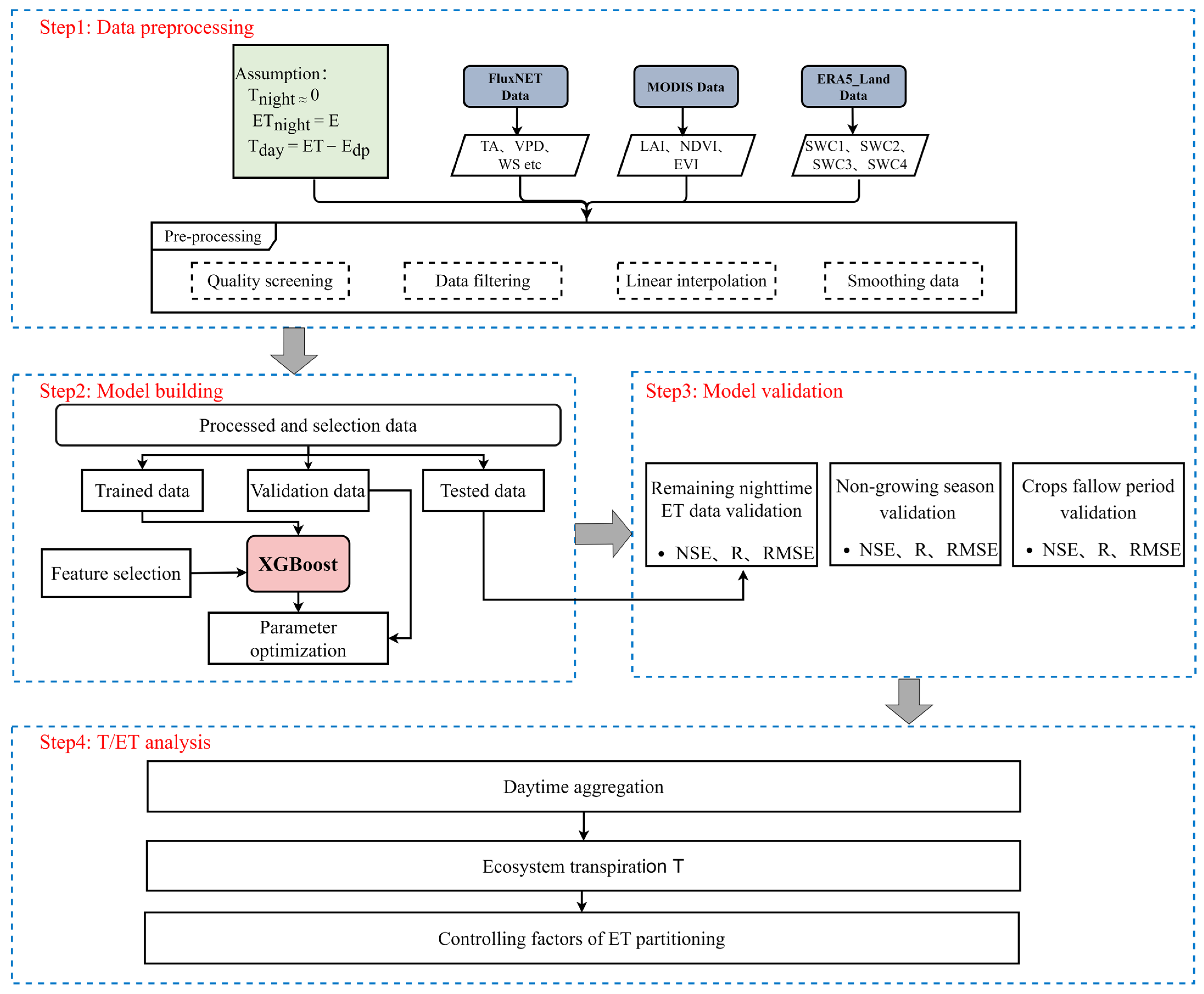
Figure 2 is the workflow of this study. Firstly, the input variables are extracted from the FLUXNET2015 dataset, MODIS dataset, and ERA5_Land dataset. Secondly, quality control is conducted on the FLUXNET2015 and MODIS data, and then data filtering is carried out on the FLUXNET2015 data. Thirdly, the MODIS data are interpolated and smoothed to be consistent with the temporal resolution of the FLUXNET2015 dataset. Finally, all of those data are separated according to their ecosystem types, and further divided into training, validation, and test datasets. After feature selection, the XGBoost model uses the training dataset for training the model. The validation dataset is used for parameter optimization to improve the model performance, and the test dataset is applied to evaluate the accuracy of the model. The T predicted by the XGBoost model is aggregated hourly to daily, and then the T/ET results are analyzed. Finally, the ET and estimated T data convert their units from W/m2 to mm/half-hour based on the following formula, and they are then aggregated at a daily scale to examine their temporal variability [33]:
E T = L E 2.501 0.002361 × T A × 10 6 × 1800
where 1800 is the time conversion coefficient of half hour, and T A is the air temperature.

2.2.2. Extreme Gradient Boosting

XGBoost is a novel machine learning algorithm introduced by Chen and Guestrin [34] that combines multiple classification and regression trees in a gradient boosting framework. XGBoost employs a parallel processing strategy and facilitates rapid training even with large datasets. Although the relationship between trees in XGBoost is serial, nodes of the same grade can be executed in parallel, making it suitable for handling extensive datasets. The fundamental concept behind the XGBoost algorithm is constantly adding trees and expanding them through performing feature splitting. After the training is completed, a collection of n trees is received, and then the prediction is made to obtain the score of a sample. Ultimately, the scores associated with each tree are summed to obtain the predicted value for this sample. As extreme gradient boosting is based on a tree model, the model was trained multiple times, where the value of the maximum depth of each tree (max_depth) was set from 1 to 1000 to minimize overfitting during the model training process. The optimal max_depth value is determined by analyzing R values obtained from the training and test datasets.

2.2.3. Feature Selection

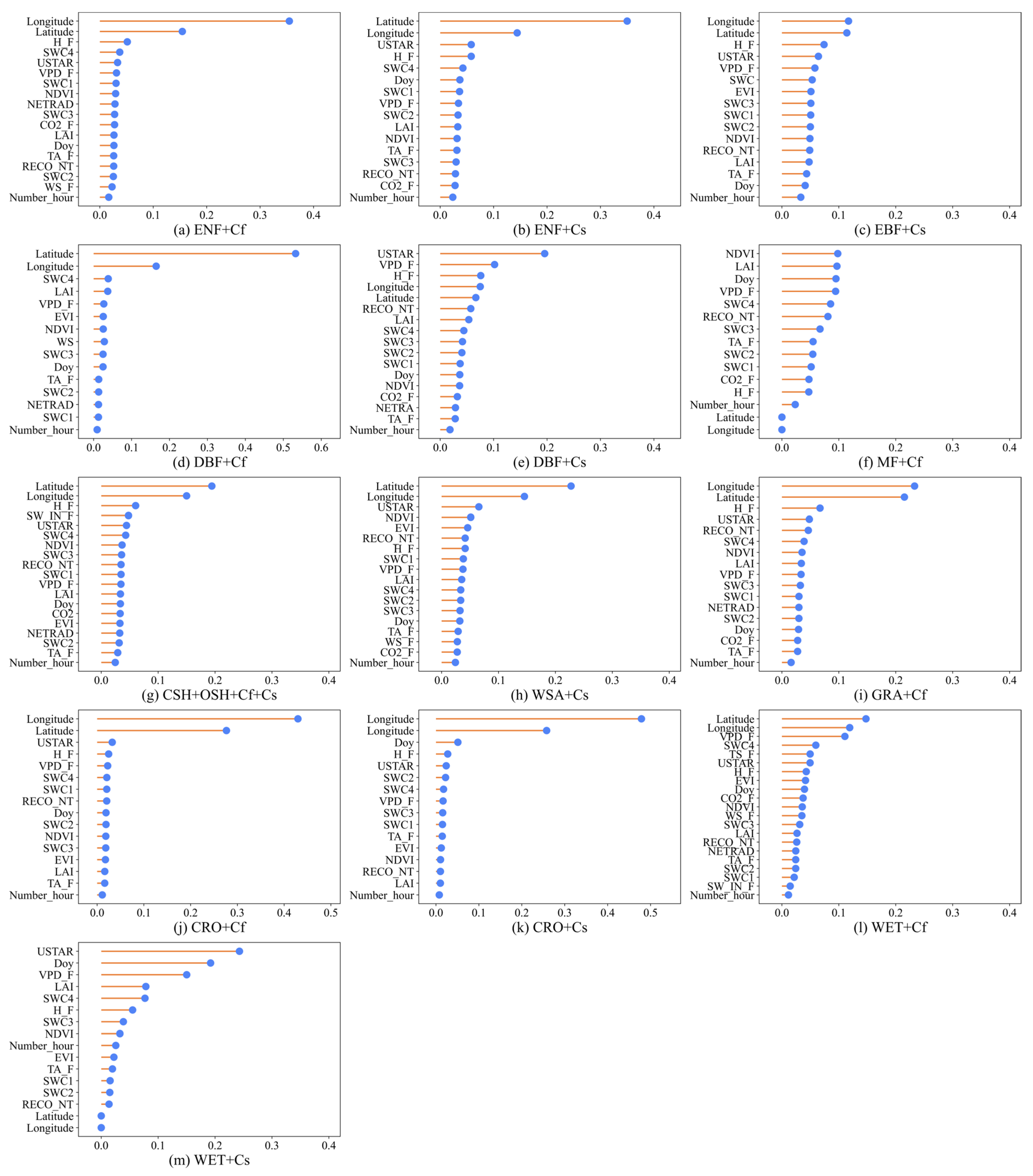
In the XGBoost algorithm, we used the feature importance to show how much each feature contributes to the model’s predictions. To obtain a better performance of the XGBoost in soil evaporation estimation, we evaluated the importance of different model input variables to find an optimal feature combination for each ecosystem. The gain value also indicates the average training loss that was decreased by using a feature [35]. Taking the feature k = 1, 2, …, K as an example, its importance can be expressed as follows:
V k = 1 2 t 1 T i 1 N t I β t , i = k G γ t , i , L 2 H γ t , i , L + λ + G γ t , i , R 2 H γ t , i , R + λ G γ t , i 2 H γ t , i + λ t = 1 T i = 1 N t I β t , i = k
where k represents a node, T represents the number of all trees, N t represents the number of non-leaf nodes in the t -th tree, β t , i represents the partition feature of the i-th non-leaf node of the t -th tree, so the β . 1 , 2 , , K . I . is the indicator function. G γ t , i and H γ t , i represent the sum of the first and second derivatives of all samples falling on the i -th non-leaf node of the t-th tree, respectively. G γ t , i , L and G γ t , i , R represent the sum of the first derivatives on the left and right nodes of the i -th non-leaf node on the t -th tree, respectively. In a similar way, H γ t , i , L and H γ t , i , R represent the sum of the second derivatives on the left and right nodes of the i -th non-leaf node on the t -th tree, respectively. λ is the hyperparameter of the regularization term.

2.2.4. Parameter Optimization

In this paper, the parameters of the XGBoost model are optimized using both random search and grid search. Random search randomly selects a set of hyperparameters from the hyperparameter space and evaluates the performance of the XGBoost model. This process is repeated multiple times to identify the optimal parameter combination. Compared with other optimization methods, random search offers the advantages of simplicity, ease of implementation, and efficient performance, mainly when dealing with a large number of hyperparameters. However, it may spend time evaluating suboptimal parameter combinations as it does not consider the interactions between hyperparameters. Grid search [36] is a traditional hyperparameter optimization method that exhaustively searches for the best hyperparameter combination by evaluating all possible combinations within the hyperparameter space.
Building a soil evaporation model with XGBoost is relatively straightforward. However, improving its accuracy through parameter tuning can be challenging. The XGBoost algorithm has multiple parameters that require optimization to enhance the model’s performance. The number of decision trees (n_estimators) and the max_depth are very important parameters of the XGBoost model. The value of n_estimators is associated with the model’s complexity, and max_depth controls the depth of the tree structure. Setting n_estimators too low may result in underfitting while setting it too high can lead to an overly complex model. Therefore, parameter adjustment requires selecting an appropriate value that strikes a balance. On the other hand, max_depth is used to avoid overfitting. A larger value allows the model to learn more specific patterns, but training deep trees in XGBoost consumes significant memory. Consequently, it is crucial to choose a suitable value for max_depth. In the XGBoost model, max_depth, n_estimators, min_child_weight (sum of minimum sample weights), and subsample (controls the proportion of random samples taken per tree) are, respectively, measured in the ranges of 1 to 1000 at intervals of 5, 1 to 1000 at intervals of 5, 1 to 10 at intervals of 1, and 0.1 to 1.0 at intervals of 0.1 for optimization using random search. Subsequently, the optimal parameter combination is finally determined through grid search based on the results obtained from the random search. The optimal parameter combinations of the ten ecosystems based on the XGBoost model are presented in Table 1.

2.3. Model Evaluation

2.3.1. Data Set Split

For model training in different ecosystem types and climate types, we divided the datasets into training, validation, and test datasets in the proportion of 70%, 15%, and 15%, respectively. The training dataset is utilized to fit the data samples to train the model, the validation is used to optimize the model parameters to improve model prediction capability, and the test dataset is used to evaluate the performance of the training model. Besides that, ten-fold cross-validation method was applied during the training to prevent overfitting. Both input and output data were standardized to mitigate the impact on the accuracy of the ML model estimation [37].

2.3.2. Model Evaluation

We use three commonly used metrics to evaluate the performance of the XGBoost model in soil evaporation estimation at different ecosystems. The three metrics are R, NSE [38], and RMSE, respectively.
R = x = 1 n K x K x ¯ O x O x ¯ x = 1 n K x K x ¯ 2 x = 1 n O x O x ¯ 2
N S E = 1 x = 1 n K x O x 2 x = 1 n K x K ¯ 2
R M S E = x = 1 n O x K 2 n
where n is the number of samples,   K x and O x are observed values and predicted values, respectively, K x ¯   and O x ¯ are the average values of the observed and the predicted data, respectively. A larger R value implies the better model performance, and R = 1 indicates the best ability of model prediction. Similarly, a higher value of NSE also indicates better model performance. The R M S E value represents the bias between the simulated and observed values [39], with a smaller R M S E indicating better performance. Therefore, higher values of R and N S E , as well as lower R M S E , correspond to superior model performance.

2.3.3. Validation of Results

One of the key challenges in the validation of ET partitioning is the scarcity of independent evaporation or transpiration data for validation [40]. Considering there is no independent measurement of ecosystem E or T at those flux sites, we selected EC measurements from certain time periods to validate the model results indirectly. During the certain time periods, soil E or ecosystem T can be distinguished and compared with the model predicted E or T data. Overall, three validation approaches were proposed in this study. The first approach uses the remaining night-time ET data (i.e., the model test data, as stated in Section 2.3.1) to validate the model. Since this portion of the data is not utilized for model training and parameter optimization, the test data are independent and can be used to validate the model accuracy.
For natural ecosystems, we additionally validated the model performance using the ET data during the non-growing season when vegetation enters into a dormant status with little photosynthesis and T. Thus, the accuracy of the predicted daytime soil evaporation can be evaluated by using the data from the non-growing season.
With regard to croplands, we can use the data from the fallow period of the crops for model validation. The fallow periods of the cropland sites are determined by the vegetation height variable recorded in the metadata data of the FLUXNET2015 dataset. To ensure the reliability of model validation, years without fallow periods in the metadata data were excluded, and the fallow periods for each site are shown in Table A2. During the fallow period, cropland ET mainly comes from the soil evaporation. Therefore, the model accuracy in croplands can be validated by comparing the predicted E-value during the fallow period with the actual E-value.

2.4. The Impacts of LAI and VPD on the Temporal Variations in T/ET

LAI and VPD are considered to be driving factors influencing the spatial and temporal variations in T/ET. To quantify their impacts on T/ET variations, the Linde-man–Merenda–Gold (LMG) method was used in this study. This method is -recommended to assess the contribution of different drivers in a linear model [41,42], which can avoid the order effect of the dependent variables in a regression [43,44]. Through the LMG method, the total R2 can be decomposed into non-negative values for each dependent variable to represent their individual contribution. We conducted this method in R software (version 4.3.1) through the “Relaimpo” package.

3. Results

3.1. Feature Selection

The optimal feature combinations of the ten ecosystems are shown in Table 2. It is evident from Table 2 that the variable combinations of the ten ecosystems all contain five variables: VPD_F_MDS, TA_F_MDS, LAI, NDVI, and SWC (SWC1, SWC2, SWC3, SWC4).
The feature importance diagrams of the ten different ecosystems are presented in Figure 3, from which we can see that in addition to the longitude and latitude coordinates, the features of VPD, LAI, and NDVI are more important. LAI is more important in DBF, MF, GRA, and WET ecosystems. Instead, VPD is more important in ENF, EBF, and CRO ecosystems. Previous studies by Feng et al. [45] and Tang et al. [46] demonstrated that incorporating vegetation variables (e.g., LAI and plant height) in the extreme learning machine model could improve the accuracy of ET estimation in maize croplands when compared to models that relied solely on meteorological data. Tu et al. [47] reported that introducing a phenological index (characterized by LAI) into the back-propagation (BP) neural network method performed better for sap flow estimation than the model without LAI. These findings collectively indicate the significance of vegetation variables, particularly the leaf area index, in accurately estimating plant transpiration. In addition to vegetation variables, air temperature, soil moisture, and VPD also contributed considerably to improving to a certain extent the accuracy of soil E estimation.

3.2. Model Results and Validation

3.2.1. Model Performance on the Remaining Night-Time Data

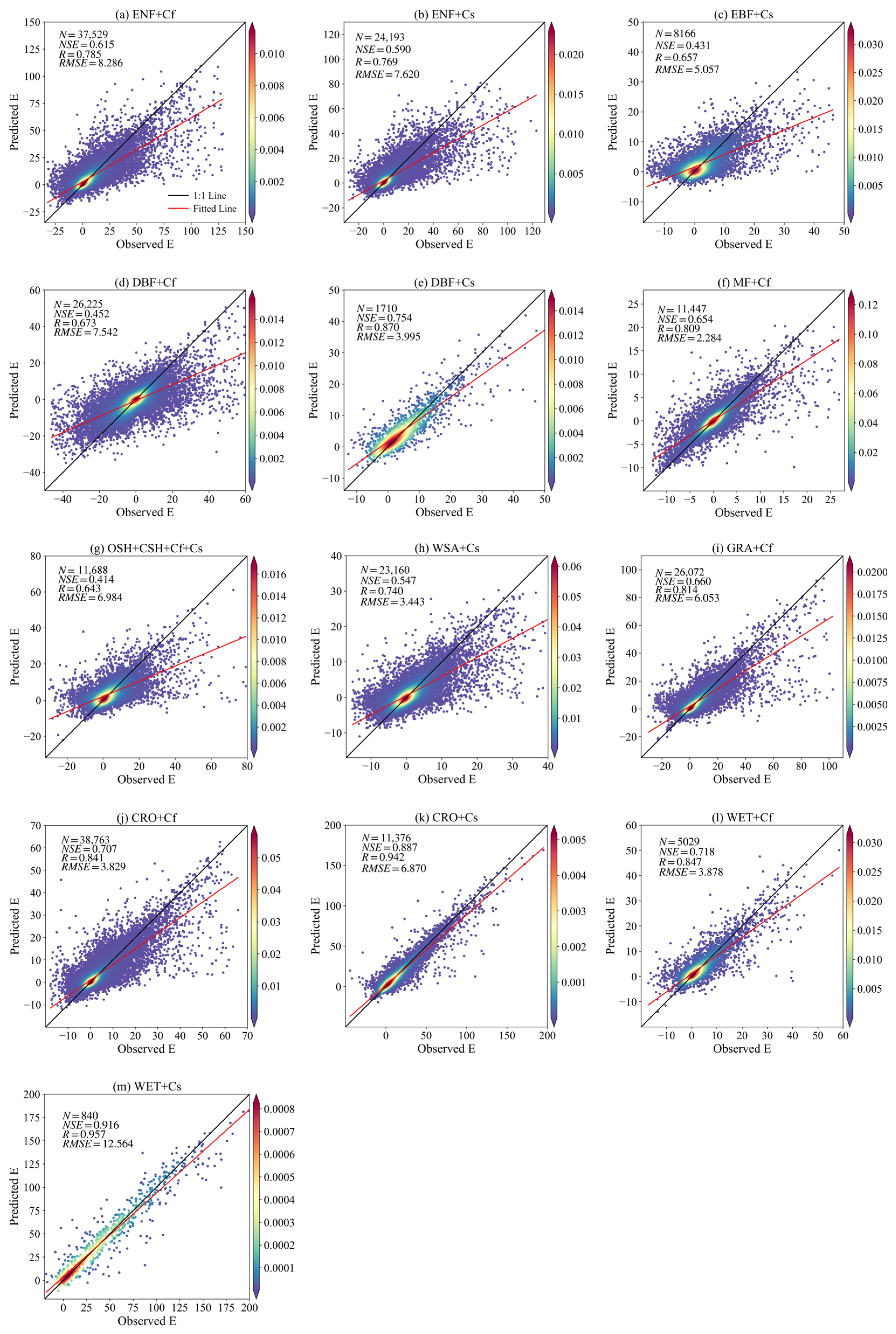
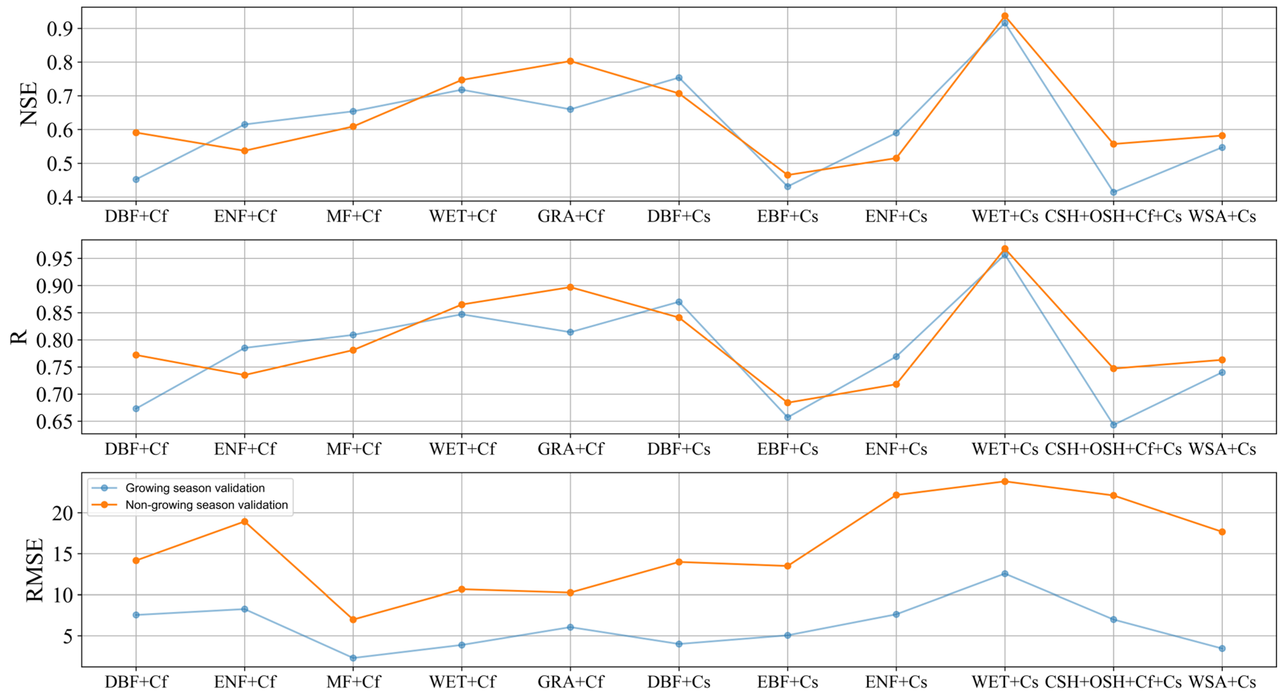
We first evaluate the accuracy of estimating E for ten different ecosystems using the remaining night-time ET data (i.e., the test dataset), and the results are presented in Figure 4 and Table 3. Notably, the prediction accuracy of different ecosystems varied considerably, with NSE values of 0.414~0.916, R values of 0.643~0.957, and RMSE values of 2.284 W/m2~12.564 W/m2. Among these, the wetland ecosystem (Figure 4l,m) generally had the best estimation accuracy with a mean NSE of 0.817, a mean R of 0.902, and a mean RMSE of 8.221 W/m2. Conversely, the shrubland ecosystem (Figure 4g) displayed the lowest estimation accuracy, with NSE of 0.414, R of 0.643, and RMSE of 6.984 W/m2. Overall, the XGBoost model could predict evaporation with acceptable accuracy for ten different ecosystems, although its accuracy could still be further enhanced in some ecosystems.

3.2.2. Validation during the Non-Growing Season

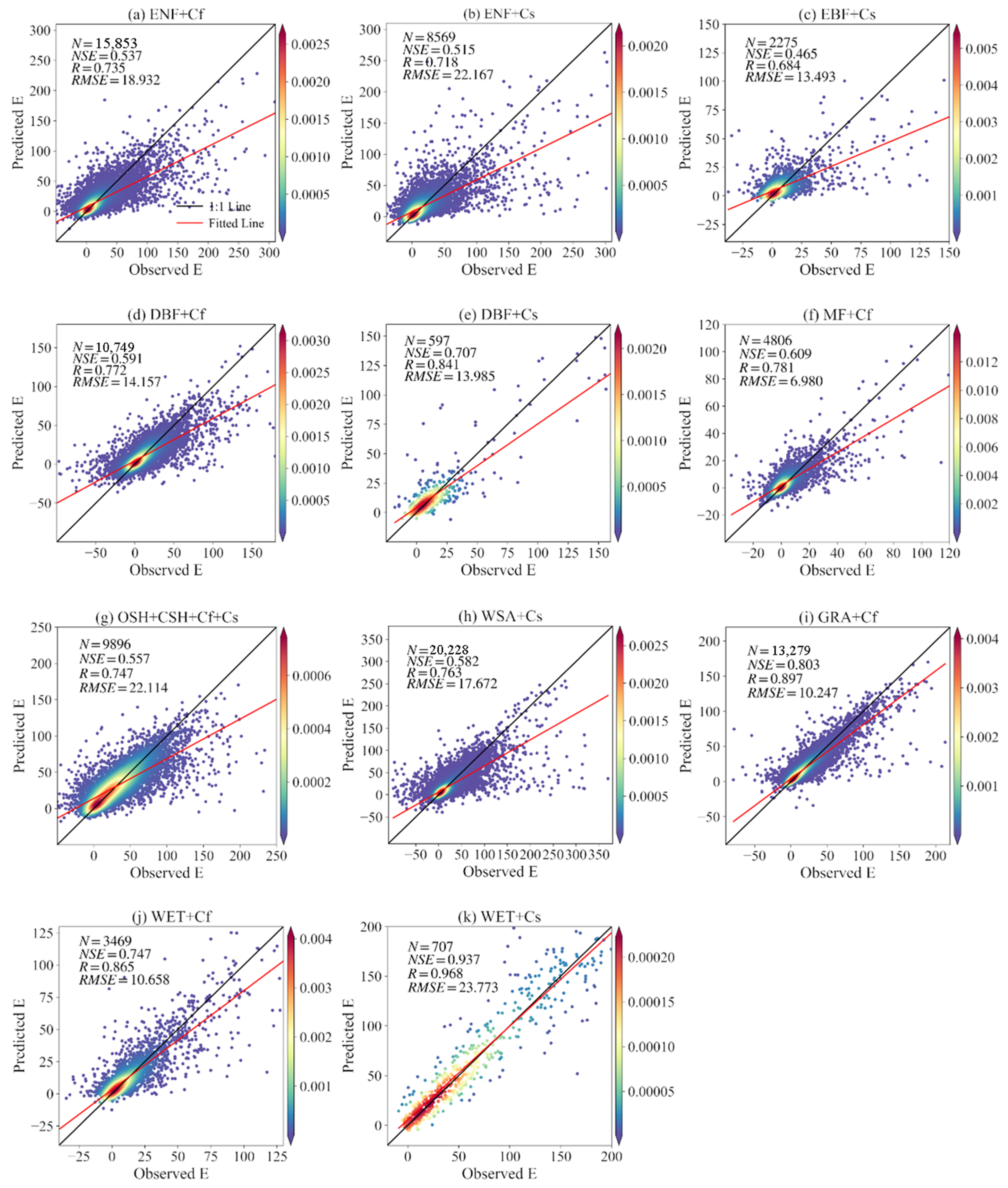
Besides validating the model using the remaining night-time ET data, we further evaluated its performance using the non-growing season ET data, and the results are presented in Figure 5. The XGBoost model exhibited notable discrepancies in performance across different ecosystems. The wetlands ecosystem still has the best model performance (Figure 5j,k), with an average NSE of 0.842, an average R of 0.917, and an average RMSE of 17.212 W/m2. However, the XGBoost model displayed a worse performance in the evergreen broadleaf forests (EBF+Cs) (Figure 5c), in which the model captured only minimal changes in E, with an average NSE of 0.465, an average R of 0.684, and an average RMSE of 13.493 W/m2. In addition, the XGBoost model performed moderately in the remaining seven ecosystems, including ENF, DBF, shrublands (OSH and CSH), MF, GRA, and WET. Compared with the accuracy from the test data, we also found that the XGBoost model demonstrated slightly better with the non-growing season data than the growing season data.

3.2.3. Validation during the Crop Fallow Period

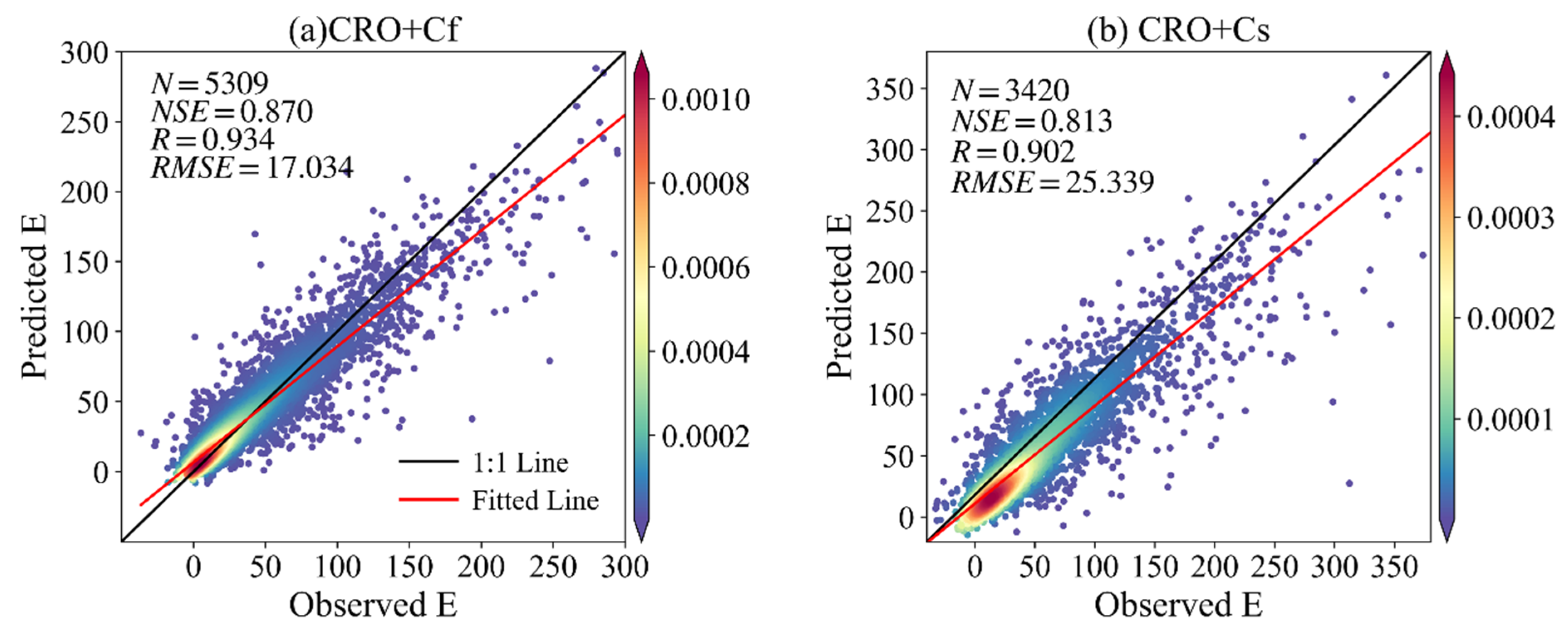
Due to the diversity and complexity of the crop rotations in the different cropland sites, its growing season for each flux site was unique and different from that of natural ecosystems. Here we mainly used its fallow period to validate the performance of the XGBoost model. In order to ensure the accuracy of the test data, years without fallow periods in the FLUXNET2015 metadata data were excluded. As shown in Figure 6, the model generally demonstrated more satisfactory performance at the cropland sites, indicated by the NSE values of 0.870–0.813, R of 0.934–0.902, and RMSE of 17.034–25.339 W/m2. Moreover, the model performed relatively better in the subtropical humid climate (Figure 6a) than in the Mediterranean climate (CRO + Cs).

3.3. Variations in ET Partitioning in Different Ecosystems

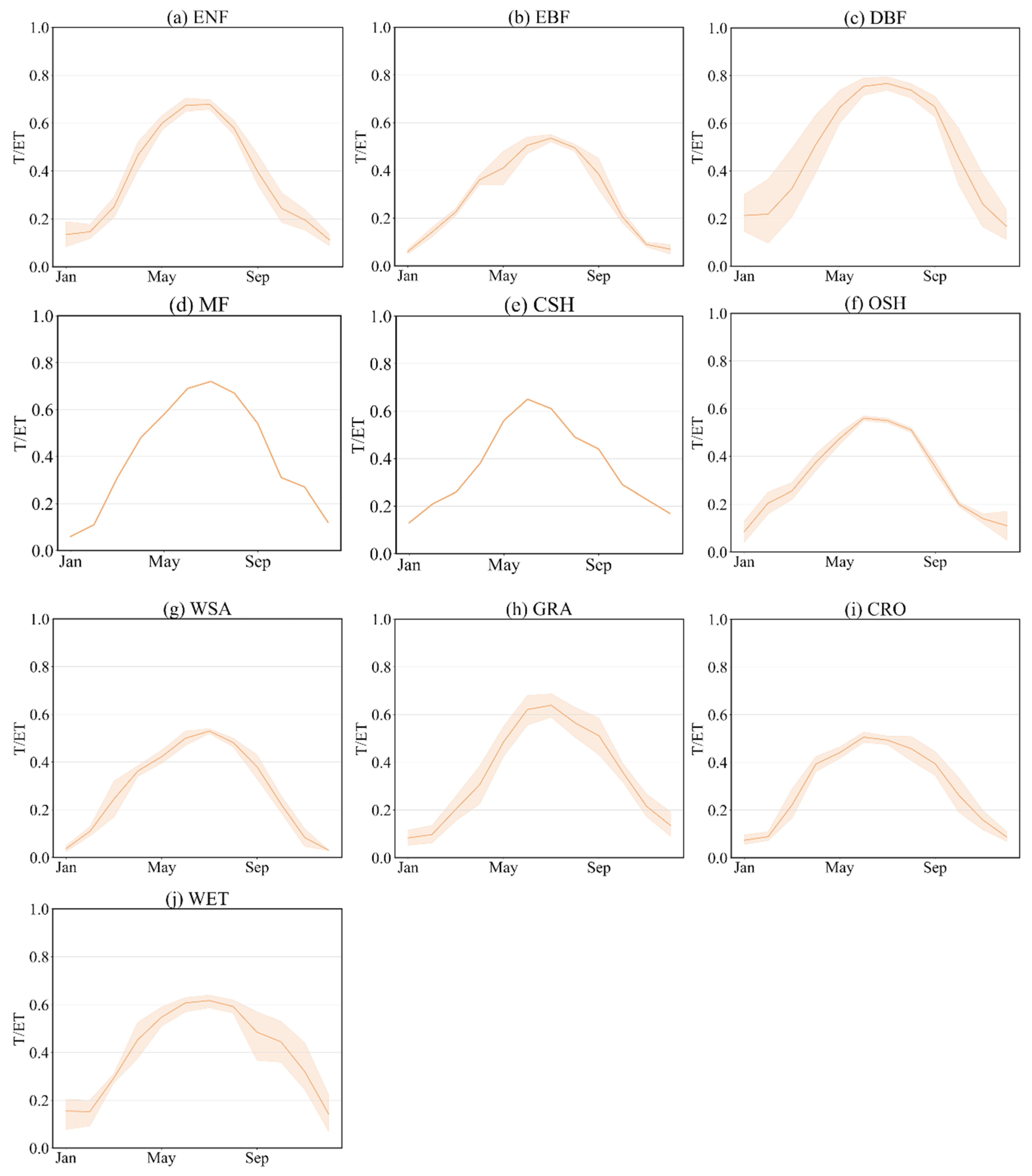
The values of T/ET between different ecosystems are presented in Figure 7. The average T/ET values among the ten ecosystems ranged from 0.4 (CRO) to 0.68 (DBF), with an average of 0.50 ± 0.08. The highest T/ET value was observed in DBF (0.68 ± 0.11), followed by MF (0.61 ± 0.04). The lowest T/ET value was found in croplands (0.40 ± 0.08), and then evergreen broadleaf forests (0.42 ± 0.04). Broadly speaking, forests generally had higher T/ET values than other ecosystems (e.g., grasslands, croplands, shrublands, and woody savannas). Among forest ecosystems, evergreen forests generally showed lower T/ET values than deciduous forests and mixed forests.
According to the ET partitioning results obtained from the XGBoost model, the seasonal variation in T/ET for the ten ecosystems is also summarized in Figure 8. As expected, T/ET in all ecosystems exhibited distinct seasonal variability, with high T/ET values during the peak of the growing season. Moreover, deciduous broadleaf forests (Figure 8c) and mixed forests (Figure 8d), showed T/ET exceeding 0.7 at the peak of the growing season. As shown in Figure 8, the growing seasons for all ten ecosystems spanned from May to August, and the peak T/ET values of evergreen needleleaf forests (Figure 8a), mixed forests (Figure 8d), and croplands (Figure 8i) were mainly observed in July and August, while the remaining ecosystems reached their peak T/ET values usually in June and July.

3.4. Effect of LAI and VPD on T/ET

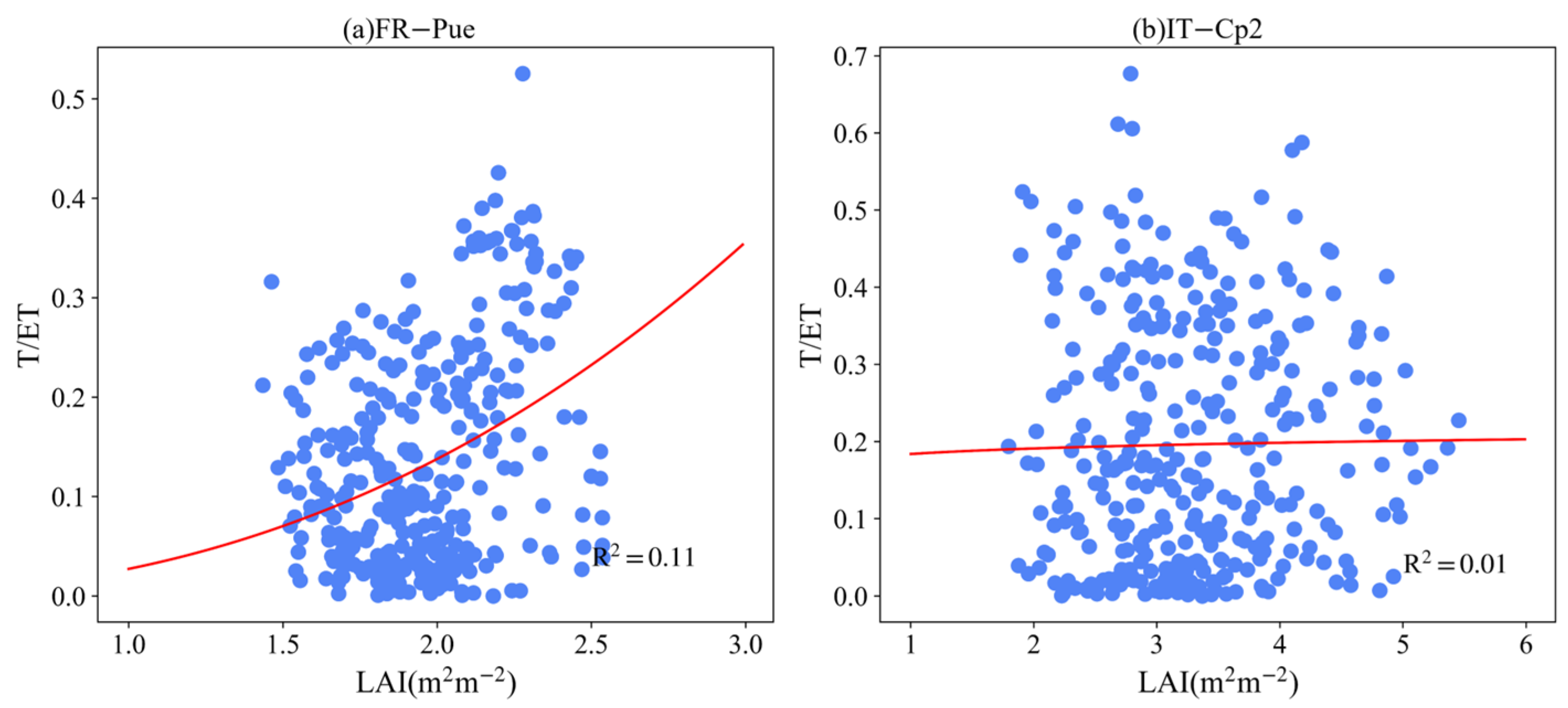
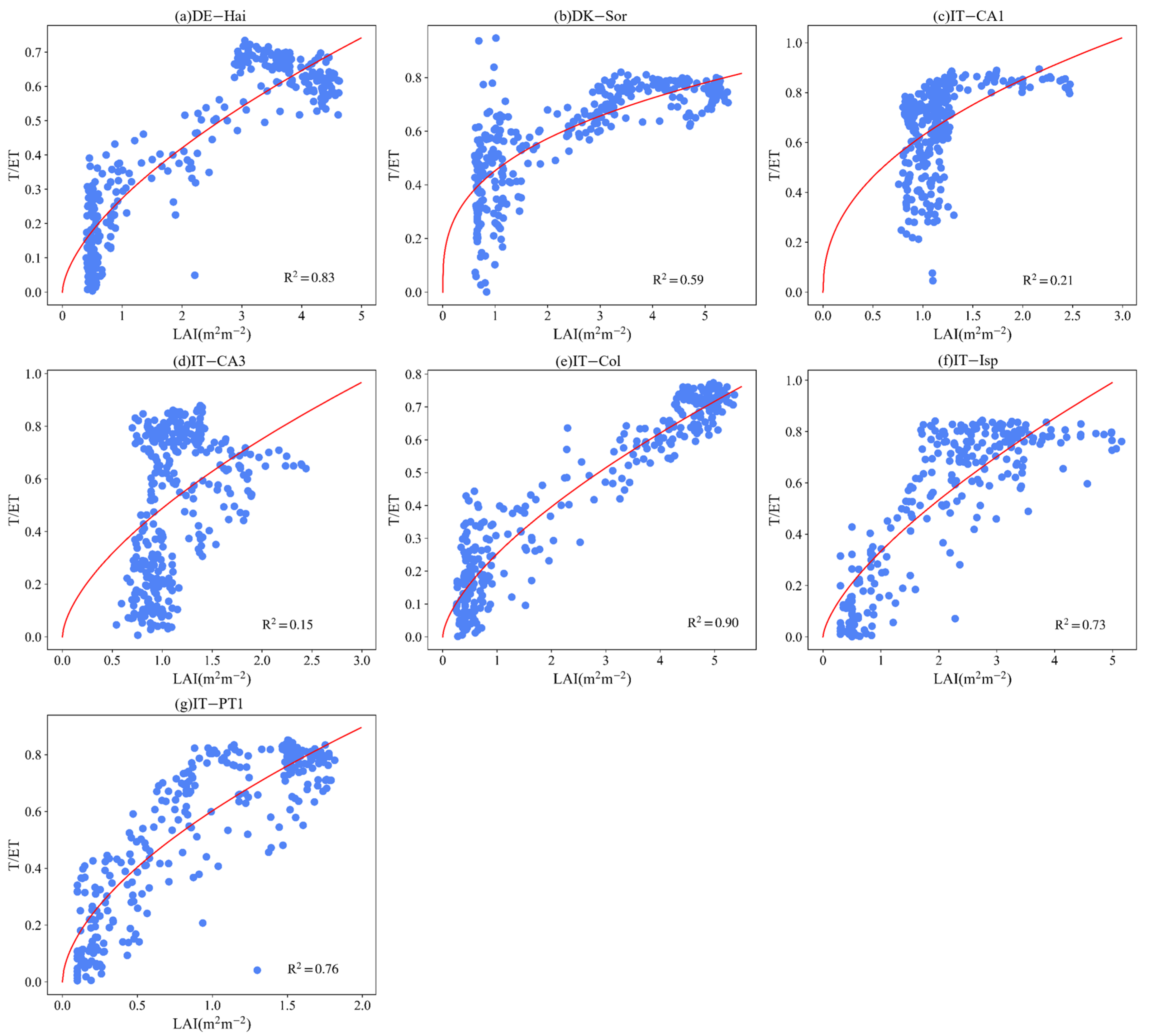
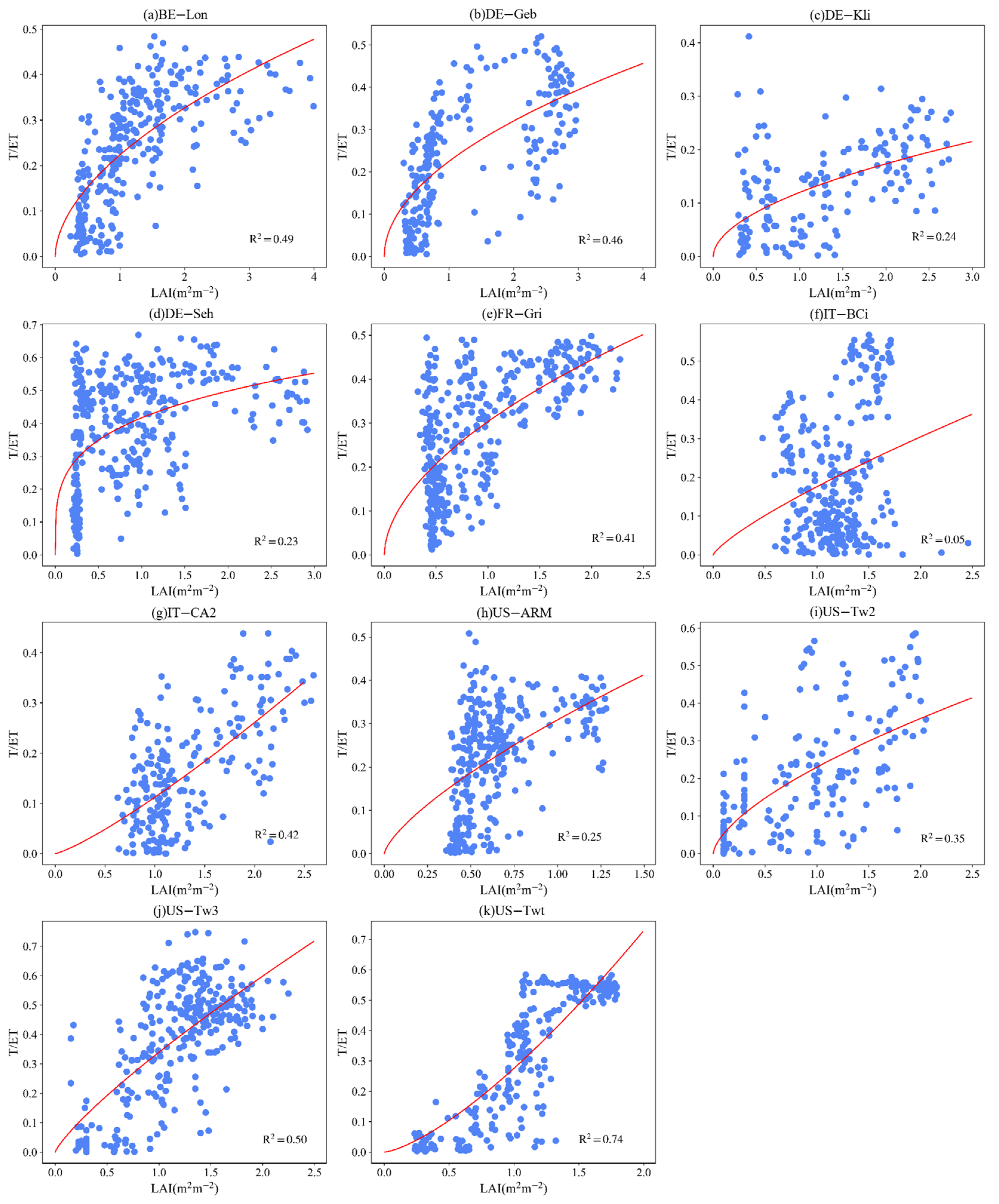
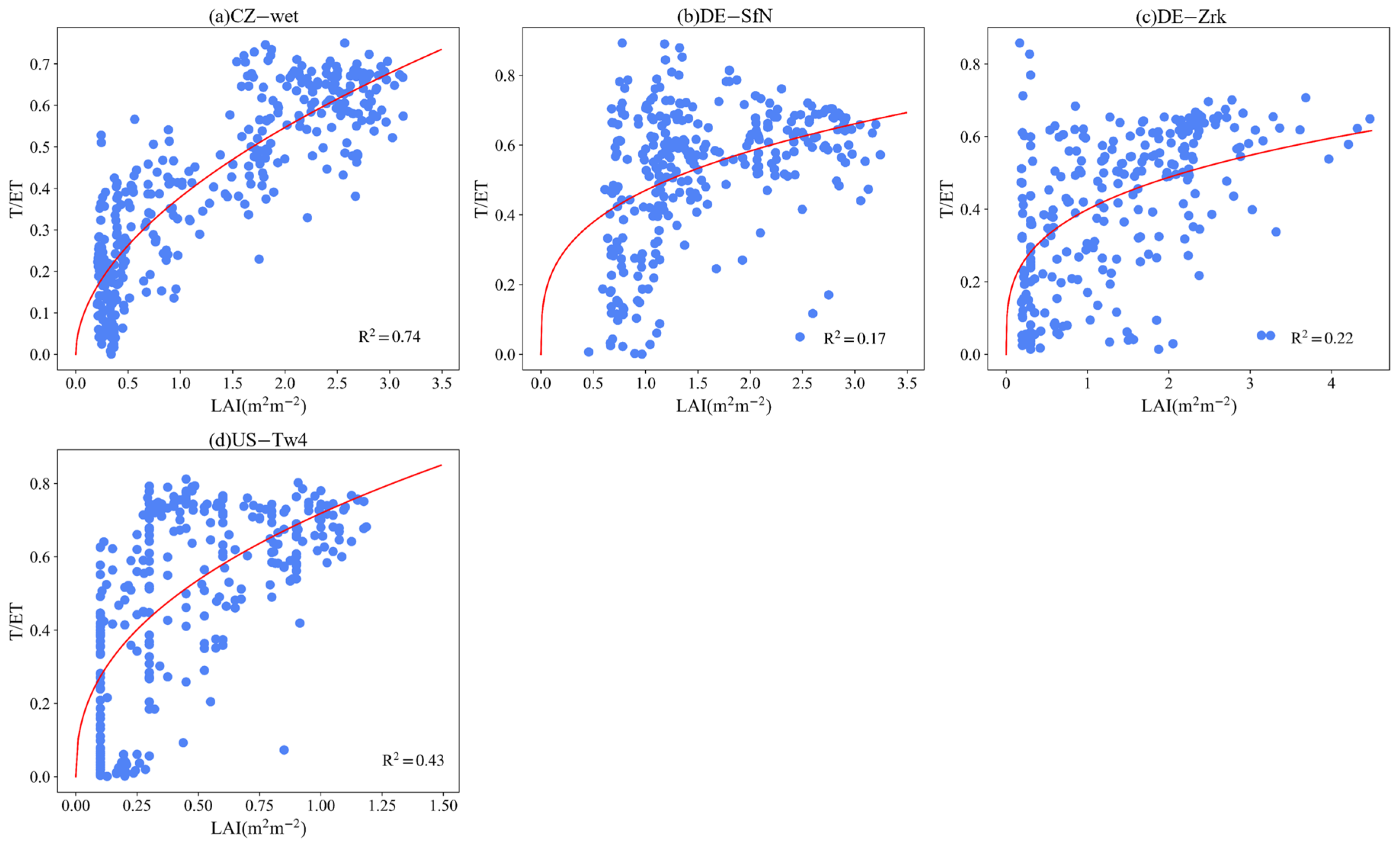
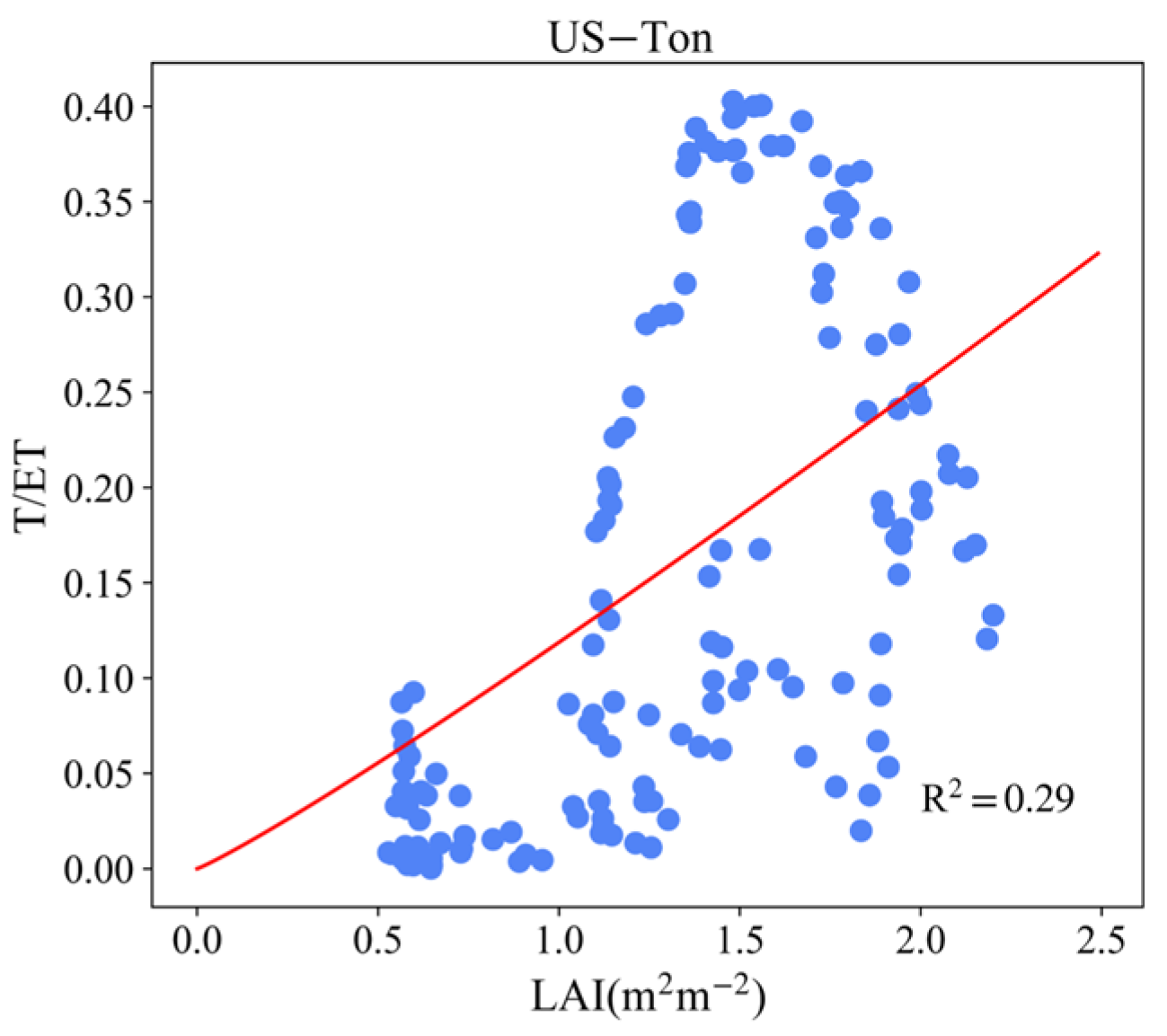
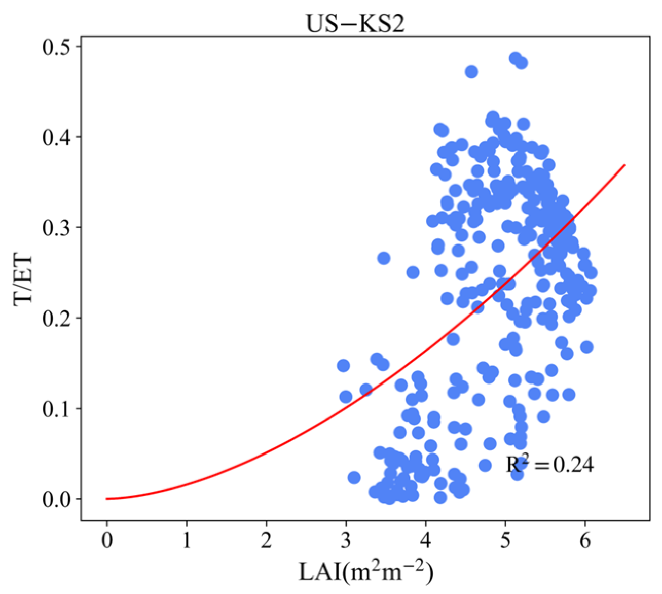
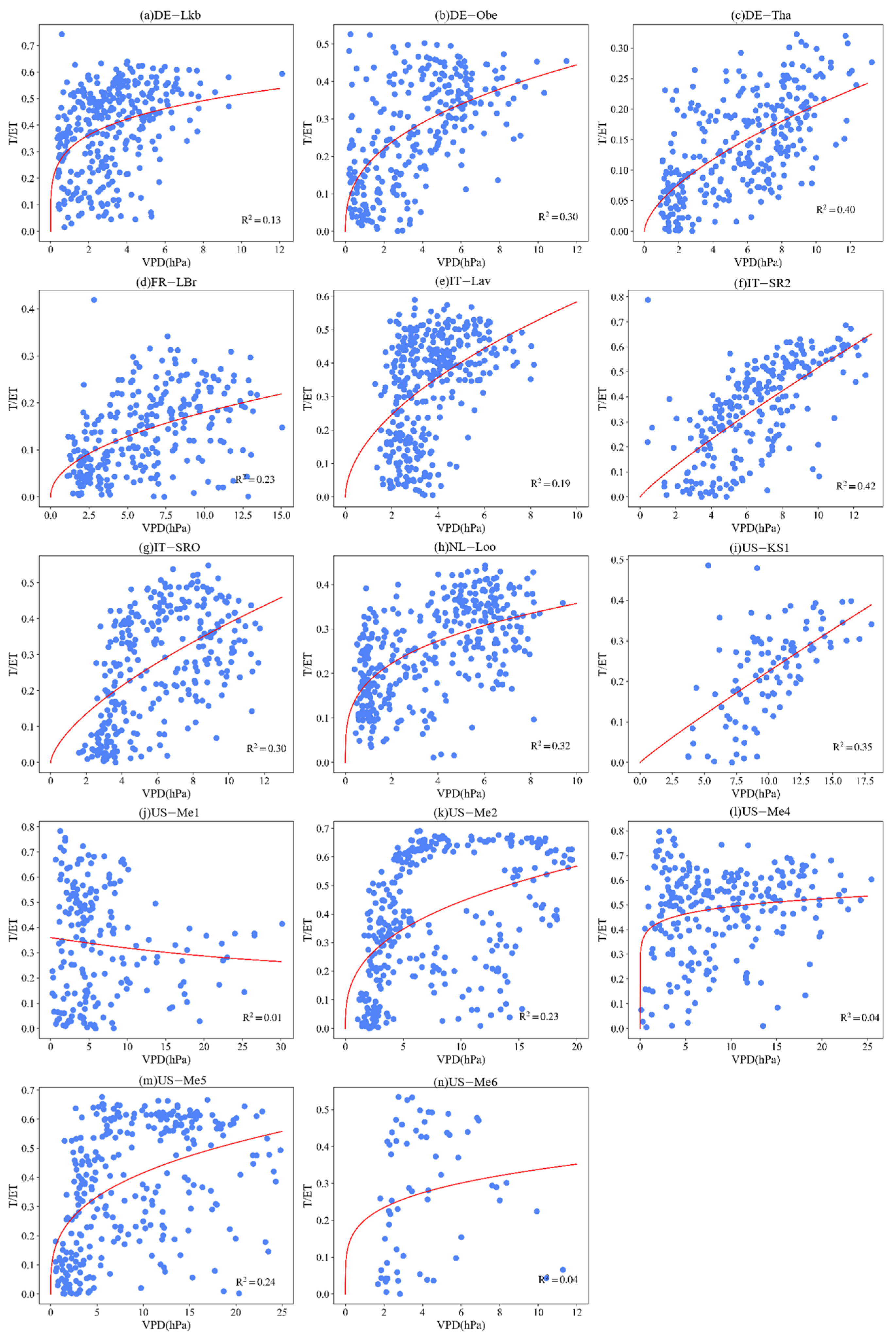
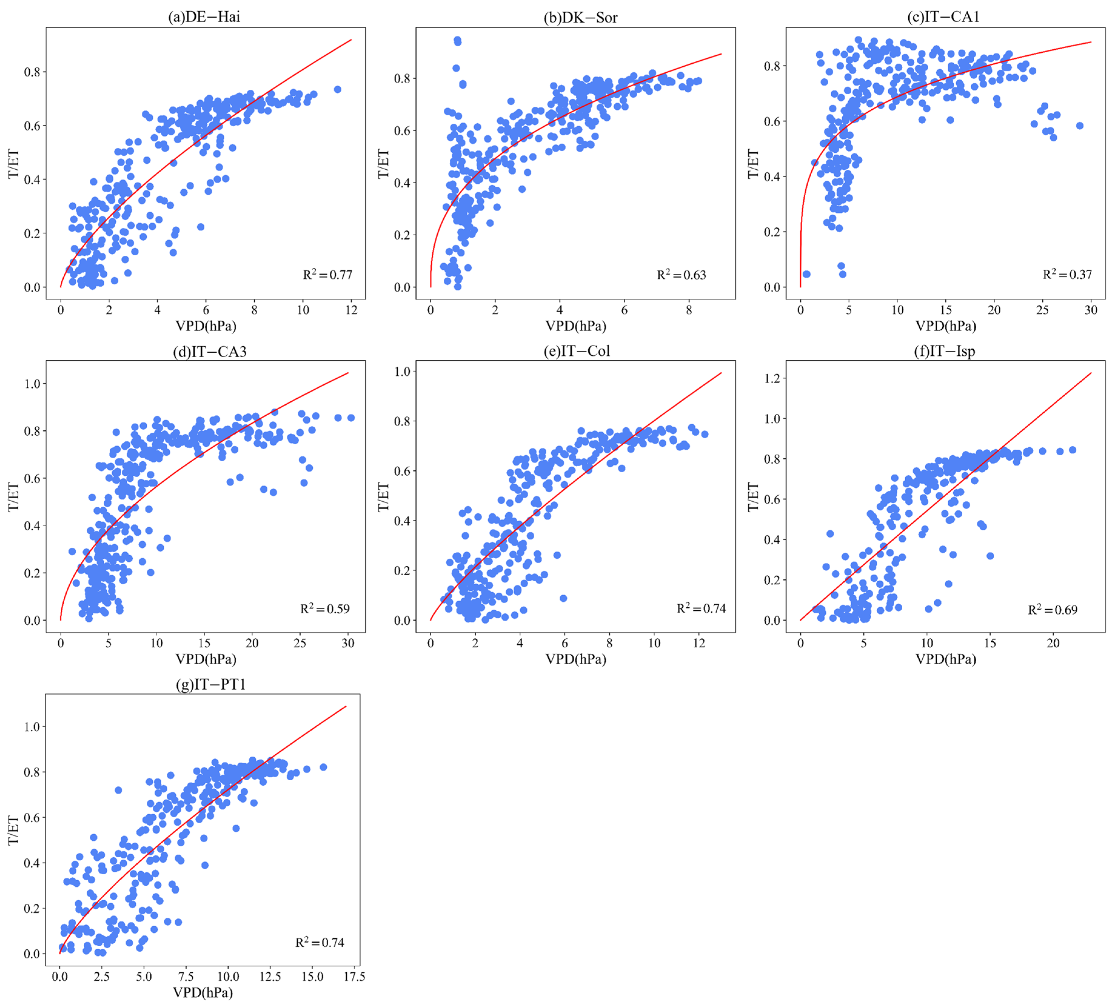
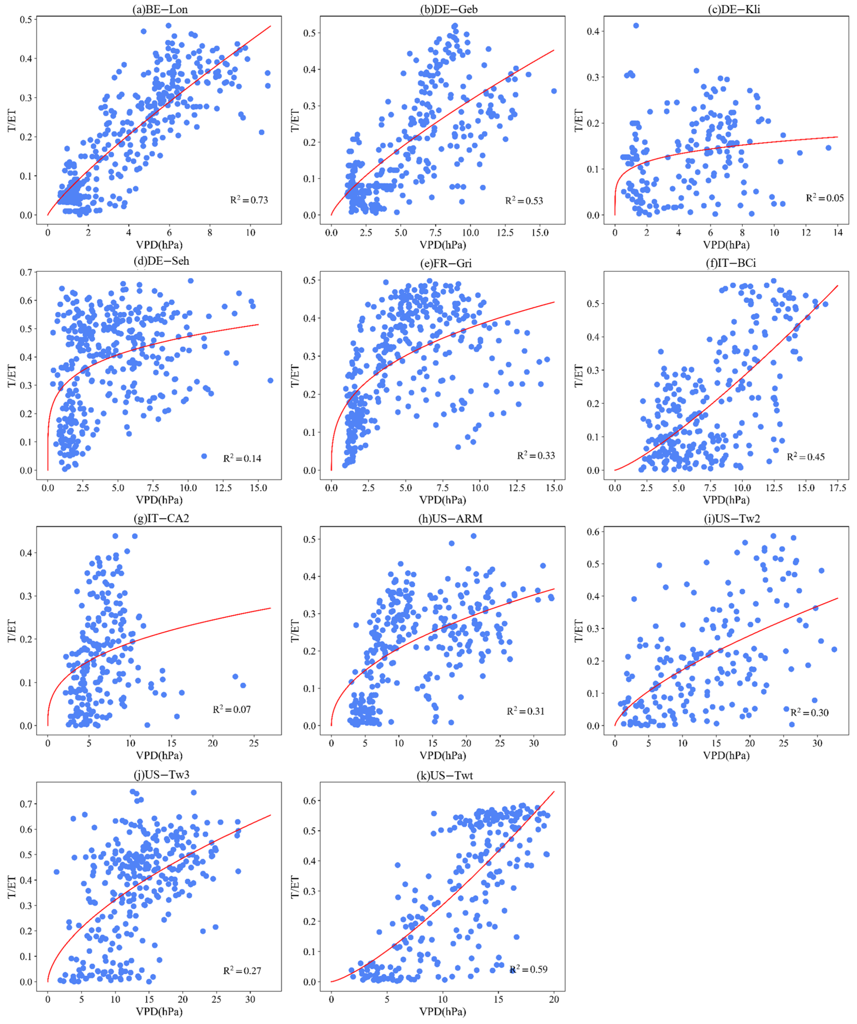
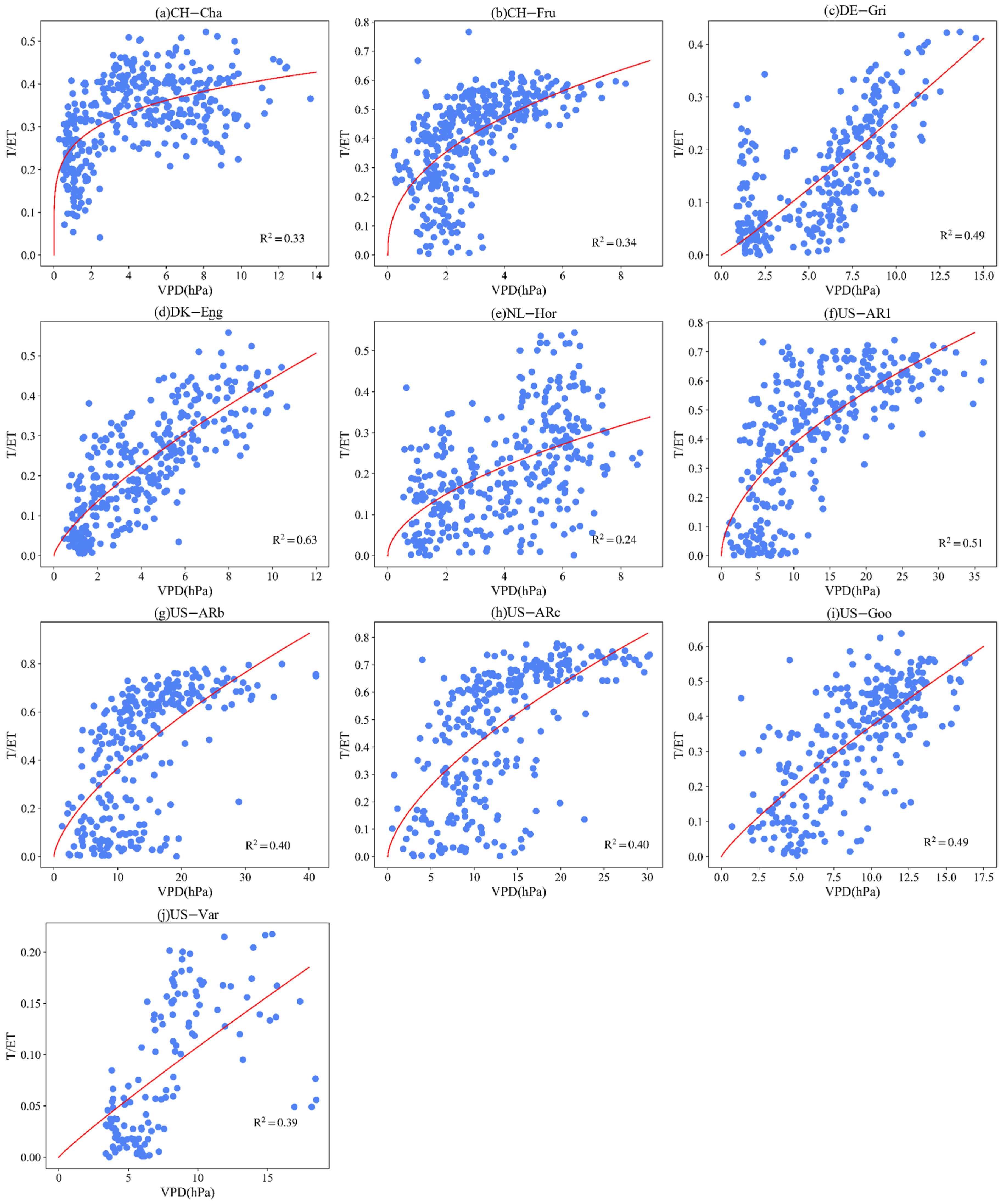
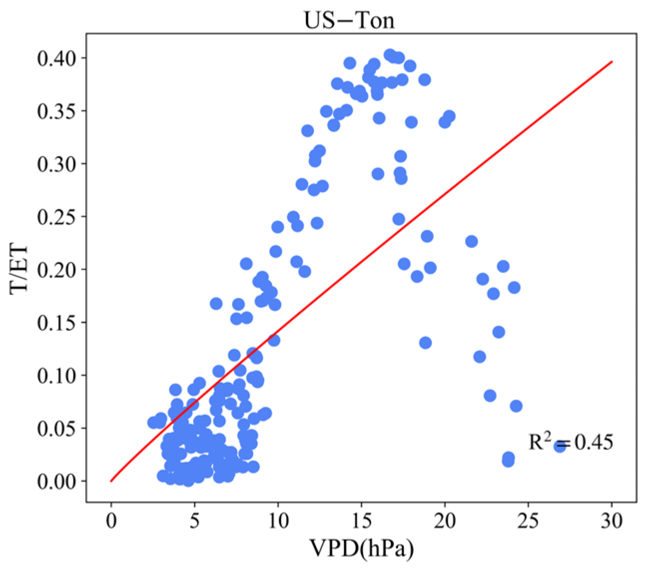
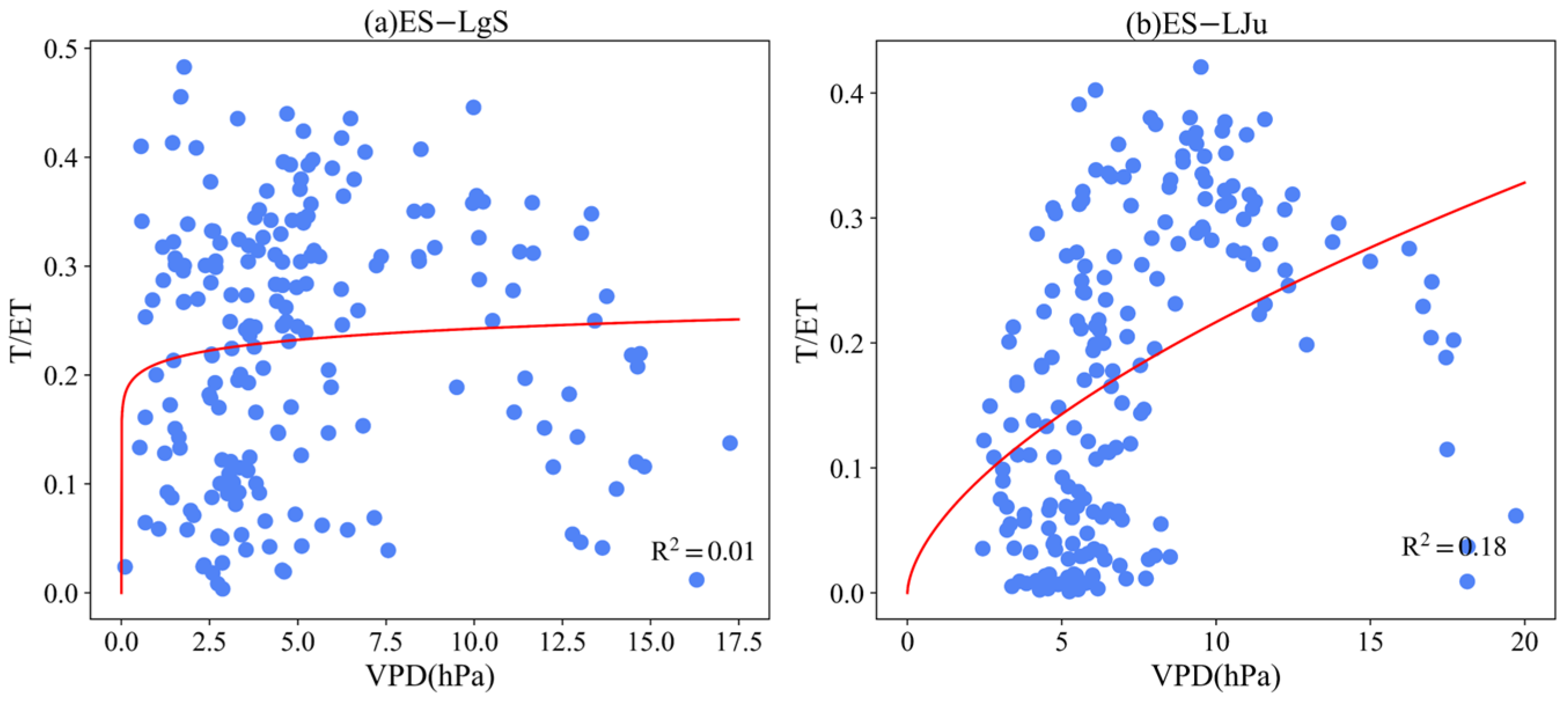
According to the analysis of feature importance shown in Section 3.1, we found that LAI and VPD had relatively greater influence on ET partitioning. Here, we furthermore examined the effects of LAI and VPD on the interannual (Figure 9) and seasonal variation in T/ET (Figure A1, Figure A2, Figure A3, Figure A4, Figure A5, Figure A6, Figure A7, Figure A8, Figure A9, Figure A10, Figure A11, Figure A12, Figure A13, Figure A14, Figure A15, Figure A16, Figure A17, Figure A18, Figure A19 and Figure A20). The results indicated that LAI played a major role in the variation in T/ET through all sites (R2 = 0.28, p < 0.001, Figure 9a), and the correlation between LAI and T/ET was stronger compared to VPD (R2 = 0.05, p < 0.001, Figure 9b). The low R2 value of 0.05 indicated that VPD had a low performance in capturing the interannual variation in T/ET, which means that VPD was not a major factor affecting T/ET variability on the interannual scale, while LAI played a more significant role. To confirm this conclusion, we further quantified the relative importance of LAI and VPD to the interannual variation in T/ET based on the LMG method (Table A3). The total explanation rate of LAI and VPD for the interannual variation in T/ET was 27%, and the explanation rates of LAI and VPD were 22% and 5%, respectively. The contribution of VPD was lower than that of LAI, which was consistent with the conclusion obtained using the regression function. We further examined the relationship between LAI (or VPD) and T/ET on the seasonal scale (Figure A1, Figure A2, Figure A3, Figure A4, Figure A5, Figure A6, Figure A7, Figure A8, Figure A9, Figure A10, Figure A11, Figure A12, Figure A13, Figure A14, Figure A15, Figure A16, Figure A17, Figure A18, Figure A19 and Figure A20) and found that T/ET increases with LAI and VPD nonlinearly. From low to middle LAI, T/ET changed dramatically, and evaporation was the main contributing factor to total ET (Figure A1, Figure A2, Figure A3, Figure A4, Figure A5, Figure A6, Figure A7, Figure A8, Figure A9 and Figure A10). After that, with the increase in LAI, T/ET increased and remained stable after reaching the maximum value, indicating that vegetation coverage controls T/ET on the seasonal scale. It was worth noting that even when LAI was at its highest, T/ET did not reach 1. For VPD, during the low-value period (Figure A11, Figure A12, Figure A13, Figure A14, Figure A15, Figure A16, Figure A17, Figure A18, Figure A19 and Figure A20), T/ET decreased rapidly, likely attributed to post-rainfall or dew periods when the surface is moist and the evaporative component of evapotranspiration is comparatively high. Similar to LAI, T/ET also increased with increasing VPD. However, after reaching a certain threshold, T/ET plateaued and exhibited a declining trend. Furthermore, when comparing the influences of LAI and VPD on T/ET at the seasonal scale (Figure A1, Figure A2, Figure A3, Figure A4, Figure A5, Figure A6, Figure A7, Figure A8, Figure A9, Figure A10, Figure A11, Figure A12, Figure A13, Figure A14, Figure A15, Figure A16, Figure A17, Figure A18, Figure A19 and Figure A20), we found that LAI also (R2 = 0.01~R2 = 0.90) had a relatively stronger impact on T/ET compared to VPD (R2 = 0.01~R2 = 0.77).

4. Discussion

4.1. Model Performances in Different Ecosystems

We observed significant differences in the performance of the XGBoost model among different ecosystems. As illustrated in Figure 10, the model exhibited the best validation results during the non-growing season (mean NSE = 0.641, mean R = 0.797, mean RMSE = 15.834 W/m2), followed by the growing season (mean NSE = 0.614, mean R = 0.779, mean RMSE = 6.155 W/m2). Specifically, in the cropland ecosystem, as shown in Table 4, the XGBoost model performed better in the fallow period (mean R = 0.918, mean NSE = 0.842, mean RMSE = 21.187 W/m2), followed by the performance in the growing season (mean R = 0.892, mean NSE = 0.797, mean RMSE = 5.350 W/m2). For the test dataset, non-growing season dataset, and fallow period dataset, excluding croplands in the Mediterranean climate, the XGBoost model tended to overestimate E when the E value was small and underestimate E when it was large (Figure 4, Figure 5 and Figure 6). The XGBoost model worked better on wetlands, deciduous broadleaf forests, and croplands, accurately modeling E with less bias, while in evergreen broadleaf forests and shrublands, the modeling results were poor. There are two possible reasons for the results. Firstly, the model may have overfitted the two ecosystems (i.e., evergreen broadleaf forests and shrublands) due to the linear interpolation of some of the data during our data processing, which resulted in excessive sample noise interference and disruption of the model learning process [48]. We set the number of iterations of the model and the number of cross-validations too high during the training of the model, which led to over-training of the model, and the model learned some noise-implicit characteristics that reduced the performance of the model. Secondly, we may have deficiencies in the feature selection process. Proper feature selection will make the model more generalizable and reduce overfitting [49], while unsuitable feature selection will lead to lower model performance. In the feature selection process of evergreen broadleaf forests and the shrublands ecosystem, the features were not selected appropriately and may have been selected to features with a low correlation with the target variable E, resulting in the reduced learning ability of the model.

4.2. The Impact of Different Machine Learning Algorithms on ET Partitioning in the CRO Ecosystem

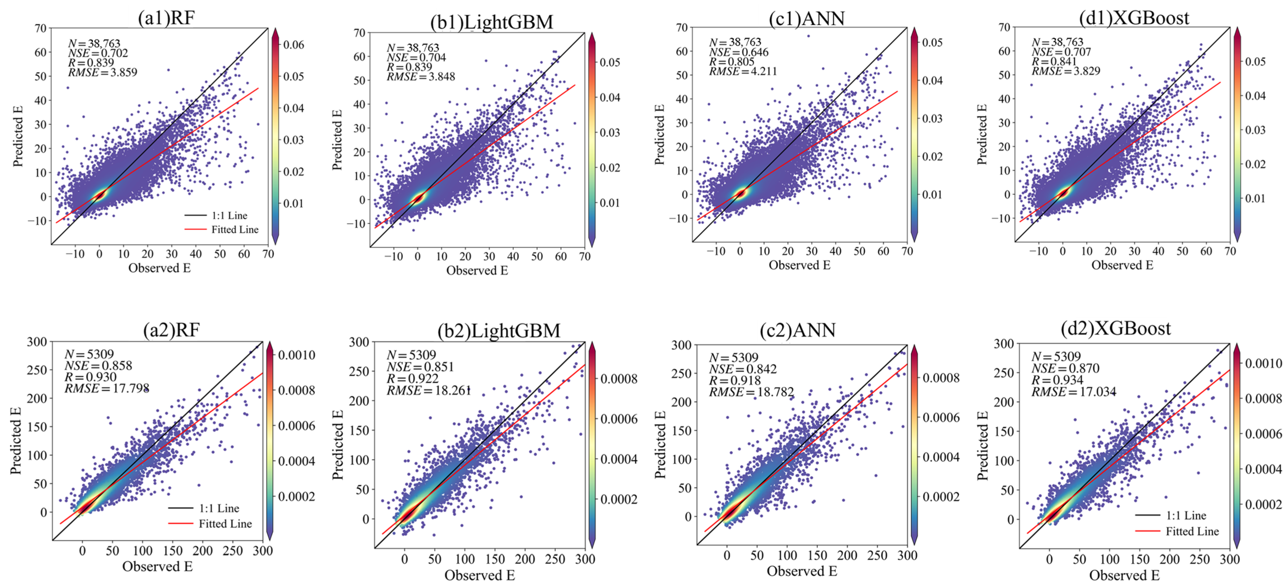
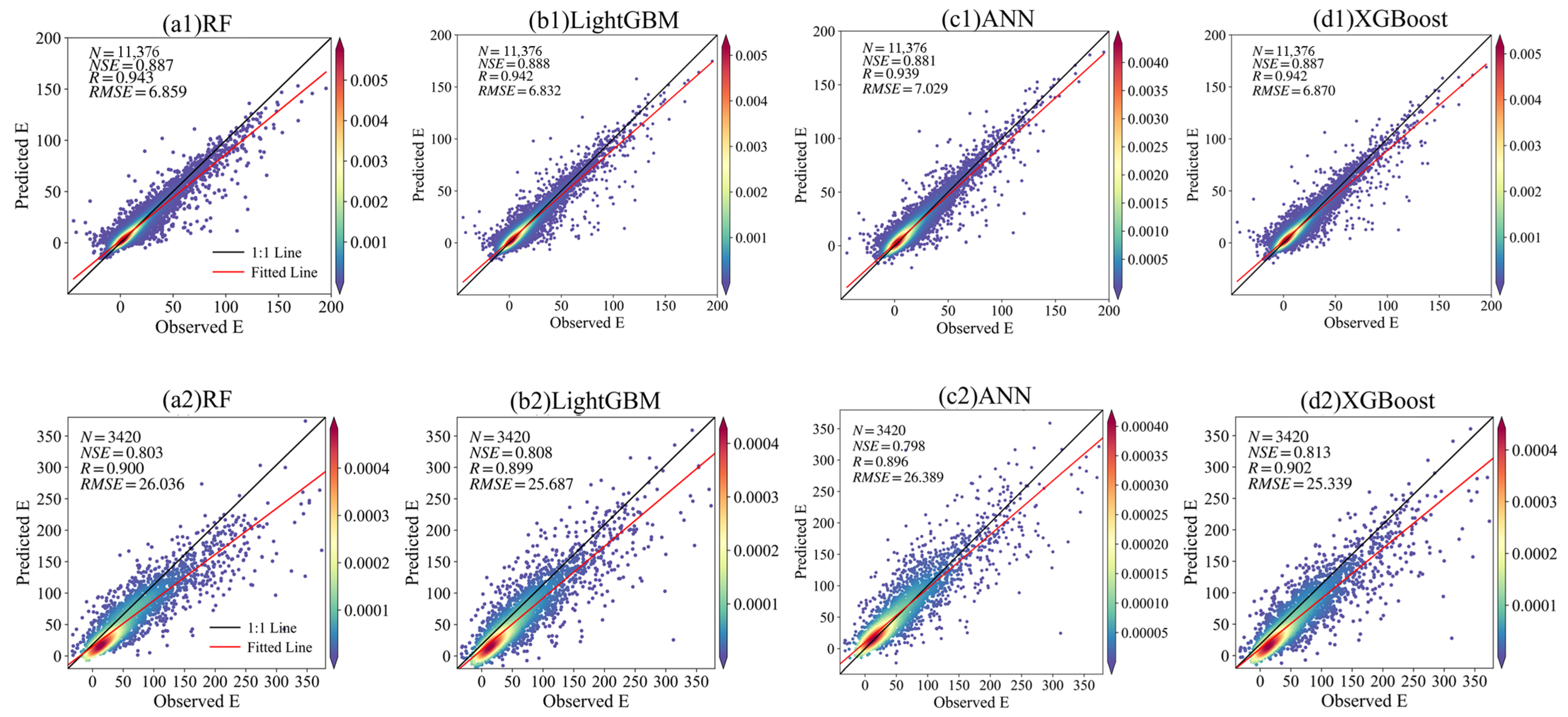
To test whether the T/ET obtained from different machine learning algorithms has a significant difference, we additionally applied the random forest (RF), light gradient boosting machine (LightGBM) algorithm, and artificial neural network (ANN) algorithm on the CRO ecosystem to compare with the XGBoost. In order to reduce the discrepancy, we employed the same training dataset, validation dataset, and test dataset, as well as the feature combinations across all models. Based on the validation results with using the remaining night-time ET data (i.e., the test dataset) (Figure 11(a1–d1) and Figure 12(a1–d1)), we found the four ML algorithms have similar performance in the CRO + Cf sites (Figure 11(a1–d1)), with NSE values of 0.646–0.707, R values of 0.805–0.841, and RMSE values of 3.829–4.211 W/m2. Similar validation results were also found in the CRO + Cs sites (Figure 12(a1–d1)), in which NSE values of the four ML algorithms varied from 0.881 to 0.888, R values varied from 0.939 to 0.943, and RMSE values varied from 17.034 W/m2 to 18.782 W/m2.
Furthermore, we evaluated the performance of the four ML using data from the crop fallow period (Figure 11(a2–d2) and Figure 12(a2–d2)). The validation results in the CRO + Cf (Figure 11(a2–d2)) and CRO + Cs sites (Figure 12(a2–d2)) confirmed that there was no significant difference between the four ML algorithms in the ET partitioning. For other ecosystems (e.g., ENF, DBF), if the four ML algorithms are well trained and parameter optimized, they would have similar accuracies in soil evaporation estimation. Nevertheless, it should be noted that the performance of the four ML algorithms is slightly different in different ecosystems, which is mainly due to the differences in ML algorithm itself and partly due to the inappropriate model training and parameter optimization.

4.3. Comparison with Other ET Partitioning Methods

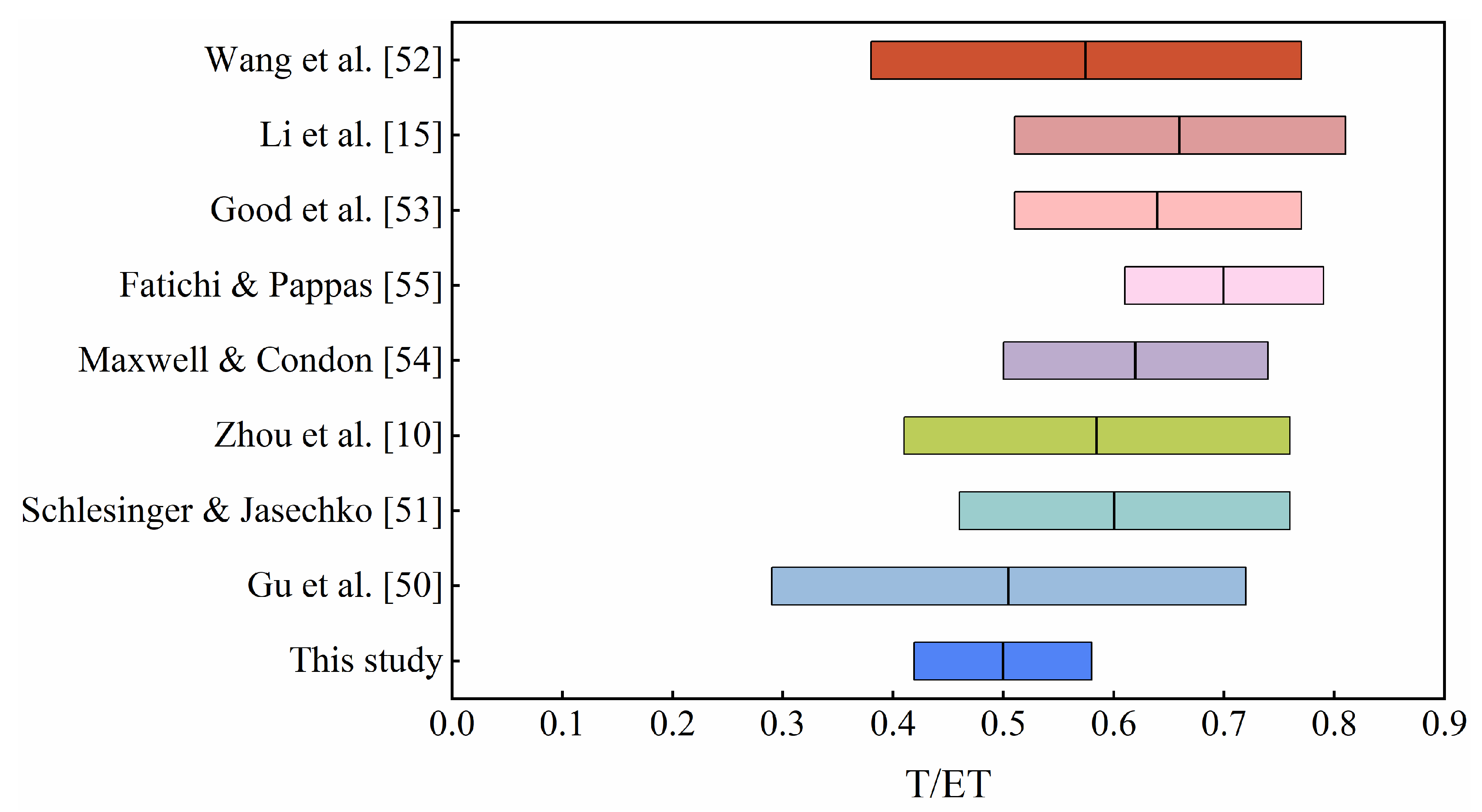
We compared the average annual T/ET for all ecosystems with previously published estimates (Figure 13) [10,15,50,51,52,53,54,55]. The mean T/ET of this study (0.50 ± 0.08) is within the range of results simulated by Gu et al. [50] (0.29~0.72), Zhou et al. [10] (0.41~0.76), and Wang et al. [52] (0.38~0.77). However, our results are slightly lower than the reported values based on isotopes, meta-analysis, and physical modeling [51,53,54]. We further compared the obtained mean annual T/ET estimates of different ecosystems with the reported values (Table 5). The annual T/ET of ENF estimated in our study (0.53 ± 0.08) is slightly lower than the values reported by Zhou et al. [10] (0.59 ± 0.06) and Schlesinger and Jasechko et al. [51] (0.55 ± 0.15). For DBF, the annual T/ET estimated by this study (0.68 ± 0.11) is very close to that of the deciduous broadleaf forests reported by Schlesinger and Jasechko et al. [51] (0.67 ± 0.14). The T/ET for GRA (0.50 ± 0.10) is also slightly below the value stated by Zhou et al. [10] (0.56 ± 0.05) and Schlesinger and Jasechko et al. [51] (0.57 ± 0.19). The T/ET range for croplands (0.40 ± 0.08) is below the value obtained by Li et al. [15] (0.62 ± 0.16), and Zhou et al. [10] (0.53–0.75), but the average value of 0.40 is very similar to the average value of 0.39 obtained by Gu et al. [50]. As Wang et al. [52] discussed, variations in observations and differences between sites can contribute to large ranges in T/ET estimates, which may explain the wide variation in T/ET estimates for the same ecosystems across different studies. Therefore, our estimated average annual T/ET for four different ecosystems (ENF, DBF, CRO, GRA) are consistent with the range of previous estimates.

4.4. Controlling Factors of ET Partitioning

Various factors, including different vegetation types, soil infiltration, climatic conditions, and water table depth, can affect the spatial and temporal variations in T/ET across different ecosystems [54,56,57,58]. Since these data were unavailable for this study, no further analysis was performed in these areas. In our study, we mainly researched the influence of LAI and VPD on ET partitioning. Our results indicate that LAI was a primary factor controlling T/ET variations (Figure 9a, Table A3). Our results are in agreement with previous reports of flux measurements at a few sites [59,60,61]. For instance, Hu et al. [59] discovered that LAI was a key driver of T/ET spatial patterns in four grassland sites. Cao et al. [62] discovered that LAI was a key driver affecting spatial variation in T/ET among sites and also a key driver affecting seasonal variation in T/ET in ecosystems. The mechanism may be that large LAI promotes transpiration by increasing the canopy stomatal conductance, and inhibits evaporation by arriving at the SR reaching the soil surface and decreasing the soil surface aerodynamic conductance [63,64]. In this study, we found no significant impact of VPD on T/ET variations (Figure 9b, Table A3). Cao et al. [62] found no significant correlation between VPD and T/ET on the interannual scale, which was consistent with confirming our conclusion. Meanwhile, seasonal variations at each site had a strong dependence on LAI. From (Figure A1, Figure A2, Figure A3, Figure A4, Figure A5, Figure A6, Figure A7, Figure A8, Figure A9 and Figure A10, it can be seen that seasonal LAI had a stronger effect on DBF, MF, and GRA, and their average R2 were 0.60, 0.79, and 0.53, respectively. From Figure A11, Figure A12, Figure A13, Figure A14, Figure A15, Figure A16, Figure A17, Figure A18, Figure A19 and Figure A20, a positive relationship between T/ET and VPD is observed. This conclusion aligns with the findings of Nelson et al. [65] using the TEA and the Pérez-Priego methods. At the same time, we also found that seasonal VPD had a higher effect on DBF, MF, WSA, and WET, and their average R2 were 0.65, 0.77, 0.45, and 0.42, respectively. When comparing the impacts of LAI and VPD on T/ET at the seasonal scale (Figure A1, Figure A2, Figure A3, Figure A4, Figure A5, Figure A6, Figure A7, Figure A8, Figure A9, Figure A10, Figure A11, Figure A12, Figure A13, Figure A14, Figure A15, Figure A16, Figure A17, Figure A18, Figure A19 and Figure A20), we obtain that the effect of LAI (R2: 0.01~0.90) on T/ET is stronger than that of VPD (R2: 0.01~0.77).

4.5. Implications and Limitations

Compared to other ET partitioning methods in the literature, the XGBoost method we used to partition ET achieves relatively superior results with fewer constraints or prior knowledge, which makes it easier to apply to various environments or ecosystems. For instance, the approach proposed by Scott and Biederman [66] only works effectively when multiyear of data are present. The shortest dataset analyzed by Scott and Biederman [66] spans eight years, this is a considerable time span, limiting its applicability. Additionally, their model may not accurately partition ET in situations where climate conditions vary among sampling sites or where the water supply does not limit fluxes (such as wetlands), and needs to be confined to a relatively dry ecosystem. This is evident in the direct comparison with our method used in this study, particularly when using the shortest dataset (i.e., one year) and when validating results in the wetlands ecosystem (Figure 4l,m), which exhibits a substantial relative contribution from E. In contrast to the method proposed by Scanlon and Kustas [9], we do not need to know plant water use efficiency in advance, which is difficult to capture in practice and varies greatly from species to species under different environmental conditions. The approach of Zhou et al. [10] assumed that E did not exist at certain time periods in the time series, and therefore, water flux during these periods was based entirely on T (i.e., T = ET). However, this assumption does not hold in humid areas or areas with high groundwater levels where it is reasonable to expect the presence of E. The method proposed by Eichelmann et al. [24] had only been validated on four wetland systems, and its applicability to other ecosystems cannot be guaranteed. In our study, we provide multiple validation approaches to validate the XGBoost model, which makes us more confident that the XGBoost model we use is more credible and significant for E and T estimates for the examined ten different ecosystems. Our approach does not depend on the assumed relationship between water and carbon fluxes. It works well in a range of ecosystems dominated by T to E, offering advantages over other approaches restricted to specific ecosystems or requiring specialized input data/equipment.
In addition, because the method proposed by our study is based on each ecosystem type, it can be directly applied to the global T/ET estimation if the input data (e.g., VPD, TA, LAI, NDVI) of the XGBoost for the ecosystems are obtained. Nevertheless, one limitation of our method is that its accuracy varies among different ecosystems. For instance, the model had higher accuracy in the CRO, DBF, and WET ecosystems, and the simulation results were more credible. Meanwhile, in the EBF and shrubland ecosystems, the estimation accuracy needed to be further improved due to the limited EC sites and observations. In future studies, it is necessary to increase EC observations and improve the representativeness of flux sites, especially for the evergreen broadleaf forest and shrubland ecosystems.
However, this study has several limitations that should be acknowledged. Firstly, the method in this paper assumes that vegetation does not exhibit T at night, equating night-time ET to night-time E. In fact, the observed data based on the sap flow measurements indicate that vegetation still exhibits weak T at night, and its value is not zero. The underlying cause of this phenomenon has not been conclusively determined. Secondly, the XGBoost model performs poorly in some ecosystems (e.g., EBF), and there are three reasons for this phenomenon. The first reason is that the parameters of the model are not suitable enough, which leads to the problem of overfitting the model in those ecosystems, and the parameters of the model need to be optimized in the future to solve this problem. The second reason for the poor results is that the temporal resolution of some data is not sufficient, and we have performed linear interpolation on the data, which has affected the quality of the data itself and some noise being generated to affect the accuracy of the model. The third reason is that the features that make the model achieve the highest accuracy were not selected, and the feature selection of the model needs to be improved in the subsequent experiments. In future studies, coupling the output data from process models (e.g., PM, PMLv2, BEPS) into the XGBoost model can be considered as a better way to improve the accuracy of ET partitioning. Process models can provide T and E output as the model inputs of ML algorithms, which makes it easy for the ML algorithms to learn the temporal variations in ET components from the sub-daily to the interannual scales and provides an opportunity to improve the accuracy of ET partitioning. Thirdly, there are no measured T data for model validation, so the partitioning T value cannot be judged correctly by measured data. Fourthly, to avoid additional errors in ET partitioning, the energy closure problem is not considered in this study. However, energy closure is an important factor influencing the estimation of LE flux in the FLUXNET2015 dataset. It has been shown that the average energy balance closure value of the global flux sites is 0.84 [67], which causes some degree of impact on LE estimation and consequently ET partitioning. In the subsequent studies, ET partitioning studies based on flux sites also need to consider the uncertainty caused by the energy closure problem on T/ET estimation.

5. Conclusions

In this study, the FLUXNET2015 dataset, remote sensing dataset, and meteorological reanalysis dataset from 55 EC sites were used to simulate E and realize ET partitioning by an XGBoost machine learning model. The validation results showed that the XGBoost model had a good effect on E estimation, with the average overall accuracy of NSE 0.657, R 0.806, and RMSE 11.344 W/m2. Notably, the results of the model were the best in the wetland ecosystem (mean NSE 0.830, mean R 0.909, mean RMSE 12.718 W/m2) and the worst in evergreen broadleaf forests (mean NSE 0.448, mean R 0.671, mean RMSE 9.275 W/m2). Using the XGBoost model, we obtained the average annual T/ET values for ten ecosystems and analyzed the primary factors influencing ET partitioning. Significant variations in T/ET were observed among different ecosystems, with DBF exhibiting the highest T/ET (0.68 ± 0.11), followed by MF (0.61 ± 0.04), while croplands exhibited the lowest T/ET (0.40 ± 0.08). In this study, at the interannual scale, VPD demonstrated a low explanatory ability (R2 = 0.05) for T/ET variations across different ecosystems, while LAI exhibited a comparatively higher explanatory ability (R2 = 0.28) for T/ET variations among different ecosystems. Meanwhile, when comparing the influence of LAI and VPD on T/ET at the seasonal scale, we found that the effect of LAI (R2: 0.01~0.90) on T/ET was also stronger than that of VPD (R2: 0.01~0.77). Meanwhile, the nonlinear relationship between T/ET and LAI indicated that even when LAI was at its highest, T/ET did not reach 1, emphasizing that E cannot be ignored even when vegetation coverage is high.
This ET partitioning method provides an easy and objective way for estimating T/ET, which can be utilized to monitor ecosystem dynamics in the global network of flux towers and enable deeper insights into the global water cycle and ecosystem functions. Moreover, the derived T/ET values can be a valuable indicator for assessing water use efficiency in diverse ecosystems. Overall, this study contributes to advancing our knowledge of hydrological processes.

Author Contributions

Conceptualization, L.L. and S.Y.; methodology, L.L. and S.Y.; software, L.L. and S.Y.; validation, L.L.; formal analysis, S.Y.; investigation, L.L. and S.Y.; resources, S.Y.; data curation, L.L. and S.Y.; writing—original draft preparation, L.L.; writing—review and editing, S.Y., D.Z., J.Z. (Jie Zhang), J.Z. (Jiahua Zhang), S.Z. and Y.B.; visualization, L.L. and S.Y.; supervision, S.Y.; project administration, S.Y.; funding acquisition, S.Y. All authors have read and agreed to the published version of the manuscript.

Funding

This study is supported by the National Natural Science Foundation of China (No. 42201407 and 42101382) and the Shandong Provincial Natural Science Foundation, China (No. ZR2022QD120 and ZR2020QD016).

Data Availability Statement

The data used in the study can be downloaded through the corresponding links provided in Section 2.1.

Acknowledgments

The authors would like to thank the editors and all anonymous reviewers for their valuable comments and useful suggestions.

Conflicts of Interest

The authors declare no conflict of interest.

Appendix A

Figure A1. Relationship between average daily T/ET and average LAI at 14 sites in ENF ecosystem. Solid line is regression for the individual data points.
Remotesensing 15 04831 g0a1
Figure A2. Relationship between average daily T/ET and average LAI at 2 sites in EBF ecosystem.
Remotesensing 15 04831 g0a2
Figure A3. Relationship between average daily T/ET and average LAI at 7 sites in DBF ecosystem.
Remotesensing 15 04831 g0a3
Figure A4. Relationship between average daily T/ET and average LAI at 1 site in MF ecosystem.
Remotesensing 15 04831 g0a4
Figure A5. Relationship between average daily T/ET and average LAI at 11 sites in CRO ecosystem.
Remotesensing 15 04831 g0a5
Figure A6. Relationship between average daily T/ET and average LAI at 10 sites in GRA ecosystem.
Remotesensing 15 04831 g0a6
Figure A7. Relationship between average daily T/ET and average LAI at 4 sites in WET ecosystem.
Remotesensing 15 04831 g0a7
Figure A8. Relationship between average daily T/ET and average LAI at 1 site in WSA ecosystem.
Remotesensing 15 04831 g0a8
Figure A9. Relationship between average daily T/ET and average LAI at 1 site in CSH ecosystem.
Remotesensing 15 04831 g0a9
Figure A10. Relationship between average daily T/ET and average LAI at 2 sites in OSH ecosystem.
Remotesensing 15 04831 g0a10
Figure A11. Relationship between average daily T/ET and average VPD at 14 sites in ENF ecosystem.
Remotesensing 15 04831 g0a11
Figure A12. Relationship between average daily T/ET and average VPD at 2 sites in EBF ecosystem.
Remotesensing 15 04831 g0a12
Figure A13. Relationship between average daily T/ET and average VPD at 7 sites in DBF ecosystem.
Remotesensing 15 04831 g0a13
Figure A14. Relationship between average daily T/ET and average VPD at 1 site in MF ecosystem.
Remotesensing 15 04831 g0a14
Figure A15. Relationship between average daily T/ET and average VPD at 11 sites in CRO ecosystem.
Remotesensing 15 04831 g0a15
Figure A16. Relationship between average daily T/ET and average VPD at 10 sites in GRA ecosystem.
Remotesensing 15 04831 g0a16
Figure A17. Relationship between average daily T/ET and average VPD at 4 sites in WET ecosystem.
Remotesensing 15 04831 g0a17
Figure A18. Relationship between average daily T/ET and average VPD at 1 site in WSA ecosystem.
Remotesensing 15 04831 g0a18
Figure A19. Relationship between average daily T/ET and average VPD at 1 site in CSH ecosystem.
Remotesensing 15 04831 g0a19
Figure A20. Relationship between average daily T/ET and average VPD at 2 sites in OSH ecosystem.
Remotesensing 15 04831 g0a20

Appendix B

Table A1. General characteristics of the 55 selected eddy covariance sites in the FLUXNET2015 dataset.
Site IDLatitudeLongitudeEcosystemKoppen Climate ClassificationYearsAverage T/ET
BE-Lon50.554.74CROCf2004–20140.35
DE-Geb51.110.91CROCf2001–20140.44
DE-Kli50.8913.52CROCf2004–20140.32
DE-Seh50.876.45CROCf2007–20100.43
DK-Fou56.489.59CROCf20050.49
FR-Gri48.841.95CROCf2004–20140.38
US-ARM36.61−97.49CROCf2003–20120.31
ES-LgS37.1−2.97OSHCs2007–20090.39
ES-LJu36.93−2.75OSHCs2004–20130.44
US-KS228.61−80.67CSHCf2003–20060.50
DE-Hai51.0810.45DBFCf2000–20090.53
DK-Sor55.4911.65DBFCf2001–20090.63
IT-Col41.8513.59DBFCf2000–20140.60
IT-Isp45.818.63DBFCf2013–20140.68
IT-PT145.209.06DBFCf2002–20040.44
DE-Lkb49.1013.30ENFCf2009–20130.48
DE-Obe50.7913.72ENFCf2008–20140.43
DE-Tha50.9613.57ENFCf2000–20140.46
FR-LBr44.72−0.77ENFCf2000–20080.49
IT-Lav45.9611.28ENFCf2003–20140.52
NL-Loo52.175.74ENFCf2000–20140.46
US-KS128.46−80.67ENFCf20020.54
CH-Cha47.218.41GRACf2005–20140.46
CH-Fru47.128.54GRACf2005–20140.50
CN-HaM37.37101.18GRACf2002–20040.43
DE-Gri50.9513.51GRACf2004–20140.53
DK-Eng55.6912.19GRACf2005–20080.43
NL-Hor52.245.07GRACf2004–20110.48
US-AR136.43−99.42GRACf2009–20120.39
US-ARb35.55−98.04GRACf2005–20060.58
US-ARc35.5465−98.04GRACf2005–20060.65
US-Goo34.25−89.87GRACf2002–20060.49
BE-Vie50.315.998MFCf2000–20140.59
CZ-wet49.0214.77WETCf2009–20140.47
DE-SfN47.8111.33WETCf2012–20140.52
DE-Zrk53.8812.89WETCf2013–20140.50
IT-BCi40.5214.96CROCs2007–20120.40
IT-CA242.3812.03CROCs2011–20140.41
US-Tw238.10−121.64CROCs2012–20130.40
US-Tw338.12−121.65CROCs2013–20140.50
US-Twt38.11−121.65CROCs2009–20140.33
US-Ton38.43−120.97WSACs2001–20140.35
US-Var38.41−120.95WSACs2000–20140.50
IT-CA142.3812.03DBFCs2011–20140.73
IT-CA342.3812.02DBFCs2011–20140.72
FR-Pue43.743.60EBFCs2002–20140.41
IT-Cp241.7012.36EBFCs2012–20140.49
IT-SR243.7310.29ENFCs2013–20140.61
IT-SRo43.7310.28ENFCs2000–20100.56
US-Me144.58−121.5ENFCs2004–20050.40
US-Me244.45−121.56ENFCs2002–20140.48
US-Me444.50−121.62ENFCs20000.57
US-Me544.44−121.57ENFCs2000–20020.53
US-Me644.32−121.61ENFCs2012–20140.37
US-Tw438.10−121.64WETCs2013–20140.45
Table A2. Fallow period of the crop sites.
Site IDCrop Fallow Period
BE-Lon29 September 2004–12 November 2004, 3 August 2005–11 August 2005, 15 September 2006–21 September 2006, 5 August 2007–25 August 2007, 4 November 2008–12 January 2009, 7 August 2009–2 September 2009, 2 December 2009–9 December 2009, 5 September 2010–14 September 2010, 16 August 2011–24 August 2011, 13 October 2012–24 October 2012, 12 August 2013–23 August 2013, 15 November 2013–23 November 2013, 22 August 2014–13 September 2014
DE-Geb16 January 2001–22 January 2001, 1 September 2001–18 October 2001, 12 August 2003–3 September 2003, 10 September 2004–20 September 2004, 23 August 2005–29 August 2005, 22 November 2005–7 December 2005, 20 April 2006–3 May 2006, 1 November 2006–16 November 2006, 29 August 2007–16 September 2007, 20 August 2008–11 September 2008, 15 October 2008–12 December 2008, 27 August 2009–1 September 2009, 24 September 2009–20 October 2009, 24 August 2010–10 September 2010, 15 November 2012–24 November 2012, 8 October 2013–15 October 2013, 19 August 2014–23 August 2014
DK-Kli30 August 2005–27 September 2005, 24 October 2006–29 October 2006, 6 March 2007–12 March 2007, 26 April 2007–2 May 2007, 12 February 2008–29 April 2008, 25 August 2009–12 October 2010, 26 March 2012–2 May 2013, 25 September 2013–11 October 2013
DK-Fou12 May 2005–24 May 2005
FR-Gri31 December 2004–1 January 2005, 2 May 2005–9 May 2005, 28 September 2005–4 October 2005, 15 July 2006–17 July 2006, 29 June 2007–2 July 2007, 10 September 2008–21 September 2008, 30 July 2009–2 August 2009, 19 July 2010–23 July 2010, 3 August 2012–15 August 2012, 6 August 2013–9 August 2013, 5 August 2014–9 August 2014
US-ARM25 July 2003–29 July 2003, 28 September 2003–1 October 2003, 19 May 2004–23 May 2004, 26 October 2005–30 October 2005, 21 June 2006–3 July 2006, 10 November 2006–14 November 2006, 25 September 2008–27 September 2008, 18 June 2009–20 June 2009, 26 September 2009–30 September 2009, 28 September 2010–30 September 2010, 15 June 2011–18 June 2011, 25 October 2011–29 October 2011, 21 May 2012–9 June 2012, 10 October 2012–15 October 2012
IT-BCi2 December 2007–13 February 2008, 2 August 2008–7 September 2008, 18 November 2008–31 December 2008, 8 January 2009–18 February 2009, 2 August 2009–13 September 2009, 21 November 2009–23 December 2009, 1 January 2010–31 January 2010, 6 February 2010–18 February 2010, 2 August 2010–13 August 2010, 21 August 2010–1 September 2010, 14 September 2010–30 September 2010, 1 November 2010–9 November 2010, 11 December 2010–30 January 2011, 21 June 2011–2 August 2011, 15 October 2011–3 November 2011, 4 January 2012–11 February 2012, 1 November 2012–23 November 2012
IT-CA222 October 2012–9 November 2012
US-Twt4 April 2009–19 May 2009, 9 September 2009–21 September 2009, 4 October 2009–31 October 2009, 9 November 2009–26 November 2009, 1 January 2010–12 February 2010, 12 April 2010–7 May 2010, 21 October 2010–23 November 2010, 3 January 2011–24 February 2011, 20 April 2011–3 May 2011, 1 November 2011–30 December 2011, 15 March 2012–27 March 2012, 19 June 2012–30 June 2012, 3 November 2012–30 December 2012, 2 January 2013–16 February 2013, 5 February 2014–19 February 2014, 9 November 2014–31 December 2014
Table A3. Relative contribution of LAI and VPD to the interannual variation in T/ET.
Influencing FactorsRelative Contribution (%)R2
LAI22%27%
VPD5%

References

  1. Jung, M.; Reichstein, M.; Ciais, P.; Seneviratne, S.I.; Sheffield, J.; Goulden, M.L.; Bonan, G.; Cescatti, A.; Chen, J.; De Jeu, R.; et al. Recent decline in the global land evapotranspiration trend due to limited moisture supply. Nature 2010, 467, 951–954. [Google Scholar] [CrossRef]
  2. Dorigo, W.; Dietrich, S.; Aires, F.; Brocca, L.; Carter, S.; Cretaux, J.F.; Dunkerley, D.; Enomoto, H.; Forsberg, R.; Güntner, A.; et al. Closing the water cycle from observations across scales: Where do we stand? Bull. Am. Meteorol. Soc. 2021, 102, E1897–E1935. [Google Scholar] [CrossRef]
  3. Trenberth, K.E.; Fasullo, J.T.; Kiehl, J. Earth’s global energy budget. Bull. Am. Meteorol. Soc. 2009, 90, 311–324. [Google Scholar] [CrossRef]
  4. Lian, X.; Piao, S.; Huntingford, C.; Li, Y.; Zeng, Z.; Wang, X.; Ciais, P.; McVicar, T.R.; Peng, S.; Ottlé, C.; et al. Partitioning global land evapotranspiration using CMIP5 models constrained by observations. Nat. Clim. Chang. 2018, 8, 640–646. [Google Scholar] [CrossRef]
  5. Baldocchi, D.D.; Ryu, Y. A Synthesis of Forest Evaporation Fluxes—From Days to Years—As Measured with Eddy Covariance. In Forest Hydrology and Biogeochemistry; Ecological Studies; Springer: Dordrecht, The Netherlands, 2011; pp. 101–116. [Google Scholar]
  6. Wen, X.; Yang, B.; Sun, X.; Lee, X. Evapotranspiration partitioning through in-situ oxygen isotope measurements in an oasis cropland. Agric. For. Meteorol. 2016, 230–231, 89–96. [Google Scholar] [CrossRef]
  7. Lu, X.; Liang, L.L.; Wang, L.; Jenerette, G.D.; McCabe, M.F.; Grantz, D.A. Partitioning of evapotranspiration using a stable isotope technique in an arid and high temperature agricultural production system. Agric. Water Manag. 2017, 179, 103–109. [Google Scholar] [CrossRef]
  8. Cammalleri, C.; Rallo, G.; Agnese, C.; Ciraolo, G.; Minacapilli, M.; Provenzano, G. Combined use of eddy covariance and sap flow techniques for partition of ET fluxes and water stress assessment in an irrigated olive orchard. Agric. Water Manag. 2013, 120, 89–97. [Google Scholar] [CrossRef]
  9. Scanlon, T.M.; Kustas, W.P. Partitioning carbon dioxide and water vapor fluxes using correlation analysis. Agric. For. Meteorol. 2010, 150, 89–99. [Google Scholar] [CrossRef]
  10. Zhou, S.; Yu, B.; Zhang, Y.; Huang, Y.; Wang, G. Partitioning evapotranspiration based on the concept of underlying water use efficiency. Water Resour. Res. 2016, 52, 1160–1175. [Google Scholar] [CrossRef]
  11. Niu, Z.; He, H.; Zhu, G.; Ren, X.; Zhang, L.; Zhang, K.; Yu, G.; Ge, R.; Li, P.; Zeng, N.; et al. An increasing trend in the ratio of transpiration to total terrestrial evapotranspiration in China from 1982 to 2015 caused by greening and warming. Agric. For. Meteorol. 2019, 279, 107701. [Google Scholar] [CrossRef]
  12. Cao, R.; Hu, Z.; Jiang, Z.; Yang, Y.; Zhao, W.; Wu, G.; Feng, X.; Chen, R.; Hao, G. Shifts in ecosystem water use efficiency on china’s loess plateau caused by the interaction of climatic and biotic factors over 1985–2015. Agric. For. Meteorol. 2020, 291, 108100. [Google Scholar] [CrossRef]
  13. Zhang, Y.; Kong, D.; Gan, R.; Chiew, F.H.S.; McVicar, T.R.; Zhang, Q.; Yang, Y. Coupled estimation of 500 m and 8-day resolution global evapotranspiration and gross primary production in 2002–2017. Remote Sens. Environ. 2019, 222, 165–182. [Google Scholar] [CrossRef]
  14. Zhou, K.; Zhang, Q.; Xiong, L.; Gentine, P. Estimating evapotranspiration using remotely sensed solar-induced fluorescence measurements. Agric. For. Meteorol. 2022, 314, 108800. [Google Scholar] [CrossRef]
  15. Li, X.; Gentine, P.; Lin, C.; Zhou, S.; Sun, Z.; Zheng, Y.; Liu, J.; Zheng, C. A simple and objective method to partition evapotranspiration into transpiration and evaporation at eddy-covariance sites. Agric. For. Meteorol. 2019, 265, 171–182. [Google Scholar] [CrossRef]
  16. Nelson, J.A.; Carvalhais, N.; Cuntz, M.; Delpierre, N.; Knauer, J.; Ogée, J.; Migliavacca, M.; Reichstein, M.; Jung, M. Coupling Water and Carbon Fluxes to Constrain Estimates of Transpiration: The TEA Algorithm. J. Geophys. Res. Biogeosci. 2018, 123, 3617–3632. [Google Scholar] [CrossRef]
  17. Liuyang, Y. Evapotranspiration Partitioning Based on Leaf and Ecosystem Water Use Efficiency. Agric. For. Meteorol. 2014, 184, 56–70. [Google Scholar] [CrossRef]
  18. Jung, M.; Reichstein, M.; Margolis, H.A.; Cescatti, A.; Richardson, A.D.; Arain, M.A.; Arneth, A.; Bernhofer, C.; Bonal, D.; Chen, J.; et al. Global patterns of land-atmosphere fluxes of carbon dioxide, latent heat, and sensible heat derived from eddy covariance, satellite, and meteorological observations. J. Geophys. Res. 2011, 116, G00J07. [Google Scholar] [CrossRef]
  19. Irvin, J.; Zhou, S.; McNicol, G.; Lu, F.; Liu, V.; Fluet-Chouinard, E.; Ouyang, Z.; Knox, S.H.; Lucas-Moffat, A.; Trotta, C.; et al. Gap-filling eddy covariance methane fluxes: Comparison of machine learning model predictions and uncertainties at FLUXNET-CH4 wetlands. Agric. For. Meteorol. 2021, 308–309, 108528. [Google Scholar] [CrossRef]
  20. Kim, Y.; Johnson, M.S.; Knox, S.H.; Black, T.A.; Dalmagro, H.J.; Kang, M.; Kim, J.; Baldocchi, D. Gap-filling approaches for eddy covariance methane fluxes: A comparison of three machine learning algorithms and a traditional method with principal component analysis. Glob. Chang. Biol. 2020, 26, 1499–1518. [Google Scholar] [CrossRef]
  21. Zhao, W.L.; Gentine, P.; Reichstein, M.; Zhang, Y.; Zhou, S.; Wen, Y.; Lin, C.; Li, X.; Qiu, G.Y. Physics-Constrained Machine Learning of Evapotranspiration. Geophys. Res. Lett. 2019, 46, 14496–14507. [Google Scholar] [CrossRef]
  22. Papale, D.; Valentini, R. A new assessment of European forests carbon exchanges by eddy fluxes and artificial neural network spatialization. Glob. Chang. Biol. 2003, 9, 525–535. [Google Scholar] [CrossRef]
  23. Tramontana, G.; Migliavacca, M.; Jung, M.; Reichstein, M.; Keenan, T.F.; Camps-Valls, G.; Ogee, J.; Verrelst, J.; Papale, D. Partitioning net carbon dioxide fluxes into photosynthesis and respiration using neural networks. Glob. Chang. Biol. 2020, 26, 5235–5253. [Google Scholar] [CrossRef]
  24. Eichelmann, E.; Mantoani, M.C.; Chamberlain, S.D.; Hemes, K.S.; Oikawa, P.Y.; Szutu, D.; Valach, A.; Verfaillie, J.; Baldocchi, D.D. A novel approach to partitioning evapotranspiration into evaporation and transpiration in flooded ecosystems. Glob. Chang. Biol. 2022, 28, 990–1007. [Google Scholar] [CrossRef]
  25. Whitley, R.; Medlyn, B.; Zeppel, M.; Macinnis-Ng, C.; Eamus, D. Comparing the Penman–Monteith equation and a modified Jarvis–Stewart model with an artificial neural network to estimate stand-scale transpiration and canopy conductance. J. Hydrol. 2009, 373, 256–266. [Google Scholar] [CrossRef]
  26. Xu, S.; Yu, Z.; Ji, X.; Sudicky, E.A. Comparing three models to estimate transpiration of desert shrubs. J. Hydrol. 2017, 550, 603–615. [Google Scholar] [CrossRef]
  27. Fan, J.; Zheng, J.; Wu, L.; Zhang, F. Estimation of daily maize transpiration using support vector machines, extreme gradient boosting, artificial and deep neural networks models. Agric. Water Manag. 2021, 245, 106547. [Google Scholar] [CrossRef]
  28. Pastorello, G.; Trotta, C.; Canfora, E.; Chu, H.; Christianson, D.; Cheah, Y.W.; Poindexter, C.; Chen, J.; Elbashandy, A.; Humphrey, M.; et al. Author Correction: The FLUXNET2015 dataset and the ONEFlux processing pipeline for eddy covariance data. Sci. Data 2021, 8, 72. [Google Scholar] [CrossRef]
  29. Knauer, J.; Zaehle, S.; Medlyn, B.E.; Reichstein, M.; Williams, C.A.; Migliavacca, M.; De Kauwe, M.G.; Werner, C.; Keitel, C.; Kolari, P.; et al. Towards physiologically meaningful water-use efficiency estimates from eddy covariance data. Glob. Chang. Biol. 2017, 24, 694–710. [Google Scholar] [CrossRef]
  30. Medlyn, B.E.; De Kauwe, M.G.; Lin, Y.S.; Knauer, J.; Duursma, R.A.; Williams, C.A.; Arneth, A.; Clement, R.; Isaac, P.; Limousin, J.M.; et al. How do leaf and ecosystem measures of water-use efficiency compare? New Phytol. 2017, 216, 758–770. [Google Scholar] [CrossRef]
  31. Chen, B.; Wang, P.; Wang, S.; Ju, W.; Liu, Z.; Zhang, Y. Simulating canopy carbonyl sulfide uptake of two forest stands through an improved ecosystem model and parameter optimization using an ensemble Kalman filter. Ecol. Model. 2023, 475, 110212. [Google Scholar] [CrossRef]
  32. Muñoz-Sabater, J.; Dutra, E.; Agustí-Panareda, A.; Albergel, C.; Arduini, G.; Balsamo, G.; Boussetta, S.; Choulga, M.; Harrigan, S.; Hersbach, H.; et al. ERA5-Land: A state-of-the-art global reanalysis dataset for land applications. Earth Syst. Sci. Data 2021, 13, 4349–4383. [Google Scholar] [CrossRef]
  33. Yang, S.; Zhang, J.; Zhang, S.; Wang, J.; Bai, Y.; Yao, F.; Guo, H. The potential of remote sensing-based models on global water-use efficiency estimation: An evaluation and intercomparison of an ecosystem model (BESS) and algorithm (MODIS) using site level and upscaled eddy covariance data. Agric. For. Meteorol. 2020, 287, 107959. [Google Scholar] [CrossRef]
  34. Chen, T.; Guestrin, C. Xgboost: A scalable tree boosting system. In Proceedings of the 22nd Acm Sigkdd International Conference on Knowledge Discovery and Data Mining, San Francisco, CA, USA, 13–17 August 2016; pp. 785–794. [Google Scholar]
  35. Shin, H. XGBoost Regression of the Most Significant Photoplethysmogram Features for Assessing Vascular Aging. IEEE J. Biomed. Health Inf. 2022, 26, 3354–3361. [Google Scholar] [CrossRef]
  36. Liashchynskyi, P.; Liashchynskyi, P. Grid search, random search, genetic algorithm: A big comparison for NAS. arXiv 2019, arXiv:1912.06059. [Google Scholar]
  37. Fan, J.; Yue, W.; Wu, L.; Zhang, F.; Cai, H.; Wang, X.; Lu, X.; Xiang, Y. Evaluation of SVM, ELM and four tree-based ensemble models for predicting daily reference evapotranspiration using limited meteorological data in different climates of China. Agric. For. Meteorol. 2018, 263, 225–241. [Google Scholar] [CrossRef]
  38. Krause, P.; Boyle, D.; Bäse, F. Comparison of different efficiency criteria for hydrological model assessment. Adv. Geosci. 2005, 5, 89–97. [Google Scholar] [CrossRef]
  39. Yu, H.; Wen, X.; Li, B.; Yang, Z.; Wu, M.; Ma, Y. Uncertainty analysis of artificial intelligence modeling daily reference evapotranspiration in the northwest end of China. Comput. Electron. Agric. 2020, 176, 105653. [Google Scholar] [CrossRef]
  40. Stoy, P.C.; El-Madany, T.; Fisher, J.B.; Gentine, P.; Gerken, T.; Good, S.P.; Liu, S.; Miralles, D.G.; Perez-Priego, O.; Skaggs, T.H.; et al. Reviews and syntheses: Turning the challenges of partitioning ecosystem evaporation and transpiration into opportunities. Biogeosciences 2019, 16, 3747–3775. [Google Scholar] [CrossRef]
  41. Li, H.; Wu, Y.; Liu, S.; Xiao, J.; Meteorology, F. Regional contributions to interannual variability of net primary production and climatic attributions. Agric. For. Meteorol. 2021, 303, 108384. [Google Scholar] [CrossRef]
  42. Ding, Y.; Gong, X.; Xing, Z.; Cai, H.; Zhou, Z.; Zhang, D.; Sun, P.; Shi, H. Attribution of meteorological, hydrological and agricultural drought propagation in different climatic regions of China. Agric. Water Manag. 2021, 255, 106996. [Google Scholar] [CrossRef]
  43. Yao, Y.; Wang, X.; Li, Y.; Wang, T.; Shen, M.; Du, M.; He, H.; Li, Y.; Luo, W.; Ma, M.; et al. Spatiotemporal pattern of gross primary productivity and its covariation with climate in China over the last thirty years. Glob. Chang. Biol. 2018, 24, 184–196. [Google Scholar] [CrossRef]
  44. Fernández-Martínez, M.; Vicca, S.; Janssens, I.A.; Sardans, J.; Luyssaert, S.; Campioli, M.; Chapin, F.S., III; Ciais, P.; Malhi, Y.; Obersteiner, M.; et al. Nutrient availability as the key regulator of global forest carbon balance. Nat. Clim. Chang. 2014, 4, 471–476. [Google Scholar] [CrossRef]
  45. Cui, N.; Mei, X.; Gong, D.; Feng, Y. Estimation of maize evapotranspiration using extreme learning machine and generalized regression neural network on the China Loess Plateau. Hydrol. Res. 2017, 48, 1156–1168. [Google Scholar] [CrossRef]
  46. Tang, D.; Feng, Y.; Gong, D.; Hao, W.; Cui, N. Evaluation of artificial intelligence models for actual crop evapotranspiration modeling in mulched and non-mulched maize croplands. Comput. Electron. Agric. 2018, 152, 375–384. [Google Scholar] [CrossRef]
  47. Tu, J.; Wei, X.; Huang, B.; Fan, H.; Jian, M.; Li, W. Improvement of sap flow estimation by including phenological index and time-lag effect in back-propagation neural network models. Agric. For. Meteorol. 2019, 276–277, 107608. [Google Scholar] [CrossRef]
  48. Montesinos López, O.A.; Montesinos López, A.; Crossa, J. Overfitting, Model Tuning, and Evaluation of Prediction Performance. In Multivariate Statistical Machine Learning Methods for Genomic Prediction; Springer: Cham, Switzerland, 2022; pp. 109–139. [Google Scholar]
  49. Dokeroglu, T.; Deniz, A.; Kiziloz, H.E. A comprehensive survey on recent metaheuristics for feature selection. Neurocomputing 2022, 494, 269–296. [Google Scholar] [CrossRef]
  50. Gu, C.; Ma, J.; Zhu, G.; Yang, H.; Zhang, K.; Wang, Y.; Gu, C. Partitioning evapotranspiration using an optimized satellite-based ET model across biomes. Agric. For. Meteorol. 2018, 259, 355–363. [Google Scholar] [CrossRef]
  51. Schlesinger, W.H.; Jasechko, S. Transpiration in the global water cycle. Agric. For. Meteorol. 2014, 189–190, 115–117. [Google Scholar] [CrossRef]
  52. Wang, L.; Good, S.P.; Caylor, K.K. Global synthesis of vegetation control on evapotranspiration partitioning. Geophys. Res. Lett. 2014, 41, 6753–6757. [Google Scholar] [CrossRef]
  53. Good, S.P.; Noone, D.; Bowen, G. Hydrologic connectivity constrains partitioning of global terrestrial water fluxes. Science 2015, 349, 175–177. [Google Scholar] [CrossRef]
  54. Maxwell, R.M.; Condon, L.E. Connections between groundwater flow and transpiration partitioning. Science 2016, 353, 377–380. [Google Scholar] [CrossRef]
  55. Fatichi, S.; Pappas, C. Constrained variability of modeled T: ET ratio across biomes. Geophys. Res. Lett. 2017, 44, 6795–6803. [Google Scholar] [CrossRef]
  56. Chen, H.; Huang, J.J.; McBean, E. Partitioning of daily evapotranspiration using a modified shuttleworth-wallace model, random Forest and support vector regression, for a cabbage farmland. Agric. Water Manag. 2020, 228, 105923. [Google Scholar] [CrossRef]
  57. Moran, M.; Scott, R.; Keefer, T.; Emmerich, W.; Hernandez, M.; Nearing, G.; Paige, G.; Cosh, M.; O’Neill, P.E. Partitioning evapotranspiration in semiarid grassland and shrubland ecosystems using time series of soil surface temperature. Agric. For. Meteorol. 2009, 149, 59–72. [Google Scholar] [CrossRef]
  58. Raz-Yaseef, N.; Yakir, D.; Schiller, G.; Cohen, S. Dynamics of evapotranspiration partitioning in a semi-arid forest as affected by temporal rainfall patterns. Agric. For. Meteorol. 2012, 157, 77–85. [Google Scholar] [CrossRef]
  59. Hu, Z.; Yu, G.; Fu, Y.; Sun, X.; Li, Y.; Shi, P.; Wang, Y.; Zheng, Z. Effects of vegetation control on ecosystem water use efficiency within and among four grassland ecosystems in China. Glob. Chang. Biol. 2008, 14, 1609–1619. [Google Scholar] [CrossRef]
  60. Sun, X.; Wilcox, B.P.; Zou, C.B. Evapotranspiration partitioning in dryland ecosystems: A global meta-analysis of in situ studies. J. Hydrol. 2019, 576, 123–136. [Google Scholar] [CrossRef]
  61. Wei, Z.; Lee, X.; Wen, X.; Xiao, W.J.A.; Meteorology, F. Evapotranspiration partitioning for three agro-ecosystems with contrasting moisture conditions: A comparison of an isotope method and a two-source model calculation. Agric. For. Meteorol. 2018, 252, 296–310. [Google Scholar] [CrossRef]
  62. Cao, R.; Huang, H.; Wu, G.; Han, D.; Jiang, Z.; Di, K.; Hu, Z. Spatiotemporal variations in the ratio of transpiration to evapotranspiration and its controlling factors across terrestrial biomes. Agric. For. Meteorol. 2022, 321, 108984. [Google Scholar] [CrossRef]
  63. Schwärzel, K.; Zhang, L.; Montanarella, L.; Wang, Y.; Sun, G. How afforestation affects the water cycle in drylands: A process-based comparative analysis. Glob. Chang. Biol. 2020, 26, 944–959. [Google Scholar] [CrossRef]
  64. Beer, C.; Ciais, P.; Reichstein, M.; Baldocchi, D.; Law, B.E.; Papale, D.; Soussana, J.F.; Ammann, C.; Buchmann, N.; Frank, D.; et al. Temporal and among-site variability of inherent water use efficiency at the ecosystem level. Glob. Biogeochem. Cycles 2009, 23, 3233. [Google Scholar] [CrossRef]
  65. Nelson, J.A.; Pérez-Priego, O.; Zhou, S.; Poyatos, R.; Zhang, Y.; Blanken, P.D.; Gimeno, T.E.; Wohlfahrt, G.; Desai, A.R.; Gioli, B.; et al. Ecosystem transpiration and evaporation: Insights from three water flux partitioning methods across FLUXNET sites. Glob. Chang. Biol. 2020, 26, 6916–6930. [Google Scholar] [CrossRef]
  66. Scott, R.L.; Biederman, J.A. Partitioning evapotranspiration using long-term carbon dioxide and water vapor fluxes. Geophys. Res. Lett. 2017, 44, 6833–6840. [Google Scholar] [CrossRef]
  67. Stoy, P.C.; Mauder, M.; Foken, T.; Marcolla, B.; Boegh, E.; Ibrom, A.; Arain, M.A.; Arneth, A.; Aurela, M.; Bernhofer, C.; et al. A data-driven analysis of energy balance closure across FLUXNET research sites: The role of landscape scale heterogeneity. Agric. For. Meteorol. 2013, 171, 137–152. [Google Scholar] [CrossRef]
Figure 1. Spatial distributions of the 55 flux sites used in this study. (a,b) are detailed explanations of black box (a) and black box (b) in the figure above.
Remotesensing 15 04831 g001
Figure 2. The workflow of this study. T n i g h t represents night-time vegetation transpiration; E T n i g h t represents night-time ecosystem transpiration; E represents soil evaporation; T d a y represents daytime vegetation transpiration; E d p represents daytime soil evaporation; NSE, R, and RMSE W/m2 are the Nash–Sutcliffe efficiency coefficient, correlation coefficient, and root mean square error, respectively. They are used to evaluate the model accuracy.
Remotesensing 15 04831 g002
Figure 3. Importance of model features for the ten ecosystems.
Remotesensing 15 04831 g003
Figure 4. Performance of the XGBoost model when estimating the values of E for all ecosystems using the growing season dataset. RMSE unit: W/m2; ENF: evergreen needleleaf forests; EBF: evergreen broadleaf forests; DBF: deciduous broadleaf forests; MF: mixed forests; CSH: closed shrublands; OSH: open shrublands; WSA: woody savannas; GRA: grasslands; CRO: croplands; WET: wetlands.
Remotesensing 15 04831 g004
Figure 5. Performance of the XGBoost model when estimating the values of E for the nine ecosystems using the non-growing season dataset. RMSE unit: W/m2.
Remotesensing 15 04831 g005
Figure 6. Performance of the XGBoost model when estimating the values of E for CRO ecosystem using the crops fallow period dataset. RMSE unit: W/m2. CRO: croplands.
Remotesensing 15 04831 g006
Figure 7. T/ET values for different ecosystems. The diamonds and solid lines in the boxes indicate the mean and median values, respectively. The solid black diamonds are outliers.
Remotesensing 15 04831 g007
Figure 8. The seasonal variations in T/ET grouped by ecosystems. The line is the mean values across sites and shading area is the 95% confidence intervals.
Remotesensing 15 04831 g008
Figure 9. The impacts of mean annual LAI (a) and VPD (b) on the interannual variations in T/ET. Solid line is the regression line. R2 is the correlation coefficient, and *** is the significant level at 0.001.
Remotesensing 15 04831 g009
Figure 10. Validation results of the XGBoost model in growing season and non-growing season for nine ecosystems.
Remotesensing 15 04831 g010
Figure 11. Performance of RF, LightGBM, ANN, and XGBoost models for estimating E values in the cropland sites with the subtropical humid climate (CRO + Cf): (1) using the test dataset; (2) using the crop fallow period dataset. RMSE unit: W/m2.
Remotesensing 15 04831 g011
Figure 12. Performance of RF, LightGBM, ANN, and XGBoost models for estimating E values in the cropland sites in the Mediterranean climate (CRO + Cs): (1) using the test dataset; (2) using the crop fallow period dataset. RMSE unit: W/m2.
Remotesensing 15 04831 g012
Figure 13. The range of T/ET obtained in our study and the values published in the previous literature. Bold solid line inside the bar represents the mean T/ET for each study, while the extension of the box represents the plus or minus standard deviation, or indicates ranges reported in the published literature.(Wang et al. [52], Schlesinger and Jasechko [51], Li et al. [15], Good et al. [53], Maxwell and Condon [54], Fatichi and Pappas [55], Zhou et al. [10] and Gu et al. [50]).
Remotesensing 15 04831 g013
Table 1. Optimal parameter combination of the ten ecosystems based on XGBoost model.
EcosystemsClimatic Typen_estimatorsmax_depthSubsamplemin_child_weight
ENFCf4901200.59
Cs4301300.77
EBFCs5001670.33
DBFCf2251000.59
Cs2611270.94
MFCf720100.74
CSH + OSHCf + Cs685650.59
WSACs9693010.59
GRACf766400.69
CROCf439310.45
Cs989850.66
WETCf935100.75
Cs943120.66
Note: Cf: subtropical humid climate; Cs: Mediterranean climate.
Table 2. Optimal variable combination based on XGBoost model.
EcosystemsClimatic TypeCombination of Variables
ENFCfLongitude, Latitude, H, SWC4, USTAR, VPD, SWC1, NDVI, NETRAD, SWC3, CO2, LAI, Doy, TA, RECO_NT, SWC2, WS, Number_hour
CsLongitude, Latitude, USTAR, H, SWC4, Doy, SWC1, VPD, SWC2, LAI, NDVI, TA, SWC3, RECO_NT, CO2, Number_hour
EBFCsLongitude, Latitude, H, USTAR, VPD, SWC4, EVI, SWC3, SWC1, SWC2, NDVI, RECO_NT, LAI, TA, Doy, Number_hour
DBFCfLongitude, Latitude, SWC4, WS_F, VPD, EVI, NDVI, LAI, SWC3, Doy, TA, SWC2, NETRAD, SWC1, Number_hour
CsUSTAR, VPD, H, Longitude, Latitude, RECO_NT, LAI, SWC4, SWC3, SWC2, SWC1, Doy, NDVI, CO2, NETRAD, TA, Number_hour
MFCfNDVI, VPD, Doy, TA, SWC4, RECO_NT, SWC3, LAI, SWC2, SWC1, CO2, H, Number_hour, Longitude, Latitude
CSH + OSHCf + CsLatitude, Longitude, H, SW_IN, USTAR, SWC4, NDVI, SWC3, RECO_NT, SWC1, VPD, LAI, Doy, CO2, EVI, NETRAD, SWC2, TA, Number_hour
WSACsLatitude, Longitude, USTAR, NDVI, EVI, RECO_NT, H, SWC1, VPD, LAI, SWC4, SWC2, SWC3, Doy, TA, WS, CO2, Number_hour
GRACfLatitude, Longitude, H, USTAR, RECO, SWC4, NDVI, VPD, LAI, SWC3, SWC1, NETRAD, SWC2, Doy, CO2, TA, Number_hour
CROCfLongitude, Latitude, USTAR, H, VPD, SWC4, SWC1, RECO_NT, Doy, SWC2, NDVI, SWC3, EVI, LAI, TA, Number_hour
CsLongitude, Latitude, Doy, H, USTAR, SWC2, SWC4, VPD, SWC3, SWC1, TA, EVI, NDVI, RECO_NT, LAI, Number_hour
WETCfLatitude, Longitude, VPD, SWC4, TS, USTAR, H, EVI, Doy, CO2, NDVI, WS, SWC3, LAI, RECO_NT, NETRAD, TA, SWC2, SWC1, SW_IN, Number_hour
CsUSTAR, Doy, VPD, H, SWC4, LAI, SWC3, NDVI, Number_hour, EVI, TA, SWC1, SWC2, RECO_NT, Latitude, Longitude
Note: The above abbreviates the full name of the variable, for example, VPD_F_MDS is abbreviated VPD.
Table 3. Statistics for training, validation, and testing XGBoost model in ten different ecosystems.
EcosystemsClimatic TypeTrainingValidationTesting
NSERRMSENSERRMSENSERRMSE
CROCf0.9700.9861.2350.6940.8224.0390.7070.8413.829
Cs0.9900.9940.2400.8340.9127.8540.8870.9426.870
DBFCf0.8070.9234.4480.4340.6187.7430.4520.6737.542
Cs0.9910.9940.7830.7030.8264.2630.7540.8703.995
ENFCf0.9530.9763.0590.5830.7398.6370.6150.7858.286
Cs0.9720.9832.5440.5580.7427.8520.5900.7697.620
MFCf0.9250.9641.1050.6240.7762.4140.6540.8092.284
WETCf0.9760.9941.1640.6820.8163.9810.7180.8473.878
Cs0.9900.9931.2630.9020.93912.7130.9160.95712.564
GRACf0.9470.9822.3970.6430.8016.2110.6600.8146.053
EBFCs0.8620.9462.5410.4030.6345.3680.4310.6575.057
CSH + OSHCf + Cs0.8940.9633.0290.4010.6277.3040.4140.6436.984
WSACs0.9610.9800.9910.5320.7183.5510.5470.7403.443
Table 4. Validation results of XGBoost model in growing season and fallow period of the croplands ecosystem.
EcosystemClimatic TypeGrowing Season ValidationFallow Period Validation
NSERRMSENSERRMSE
CROCf0.7070.8413.8290.8700.93417.034
CROCs0.8870.9426.8700.8130.90225.339
Table 5. Comparison T/ET with other ET partitioning methods.
EcosystemThis StudyPublished Studies
ENF0.53 ± 0.08Zhou et al. [10] (0.59 ± 0.06)
Schlesinger and Jasechko et al. [51] (0.55 ± 0.15)
DBF0.68 ± 0.11Schlesinger and Jasechko et al. [51] (0.67 ± 0.14)
GRA0.50 ± 0.10Zhou et al. [10] (0.56 ± 0.05)
Schlesinger and Jasechko et al. [51] (0.57 ± 0.19)
CRO0.40 ± 0.08Zhou et al. [10] (0.53–0.75)
Li et al. [15] (0.62 ± 0.16)
Gu et al. [50] reported a mean value of 0.39
Disclaimer/Publisher’s Note: The statements, opinions and data contained in all publications are solely those of the individual author(s) and contributor(s) and not of MDPI and/or the editor(s). MDPI and/or the editor(s) disclaim responsibility for any injury to people or property resulting from any ideas, methods, instructions or products referred to in the content.