Article

Exploiting Temporal–Spatial Feature Correlations for Sequential Spacecraft Depth Completion

1
School of Astronautics, Harbin Institute of Technology, Harbin 150001, China
2
Qian Xuesen Laboratory of Space Technology, China Academy of Space Technology, Beijing 100080, China
*
Author to whom correspondence should be addressed.
Remote Sens. 2023, 15(19), 4786; https://doi.org/10.3390/rs15194786
Submission received: 12 August 2023 / Revised: 18 September 2023 / Accepted: 27 September 2023 / Published: 30 September 2023
(This article belongs to the Section Remote Sensing Image Processing)

Abstract

:
The recently proposed spacecraft three-dimensional (3D) structure recovery method based on optical images and LIDAR has enhanced the working distance of a spacecraft’s 3D perception system. However, the existing methods ignore the richness of temporal features and fail to capture the temporal coherence of consecutive frames. This paper proposes a sequential spacecraft depth completion network (S2DCNet) for generating accurate and temporally consistent depth prediction results, and it can fully exploit temporal–spatial coherence in sequential frames. Specifically, two parallel convolution neural network (CNN) branches were first adopted to extract the features latent in different inputs. The gray image features and the depth features were hierarchically encapsulated into unified feature representations through fusion modules. In the decoding stage, the convolutional long short-term memory (ConvLSTM) networks were embedded with the multi-scale scheme to capture the feature spatial–temporal distribution variation, which could reflect the past state and generate more accurate and temporally consistent depth maps. In addition, a large-scale dataset was constructed, and the experiments revealed the outstanding performance of the proposed S2DCNet, achieving a mean absolute error of 0.192 m within the region of interest.

1. Introduction

The proliferation of satellites in Earth’s orbit has witnessed a significant surge in recent years. However, as many satellites encounter malfunctions or deplete their fuel reserves, the need for on-orbit maintenance [1] or the recovery of critical components [2] has become imperative. During the execution of on-orbit maintenance tasks, acquiring a target’s precise three-dimensional point cloud data is paramount as these data play a pivotal role in various aspects of space operations, such as navigation [3], three-dimensional (3D) reconstruction, pose estimation [4,5], component identification and localization [6], and decision-making. Consequently, the acquisition of precise 3D point cloud data from a target object has emerged as a critical and fundamental requirement for the successful execution of numerous space missions to be conducted in the dynamic and challenging space environment.
To date, different sensor options have been proposed to obtain point cloud data efficiently and accurately, and they can be categorized into multi-camera vision systems [7], time-of-flight (TOF) cameras [8], and techniques that combine monocular and LIDAR systems [9]. Among these, multi-camera-based solutions utilize the triangulation principle to recover the depths of the extracted feature points, though these solutions struggle with smooth surfaces or repetitive textures. Furthermore, a binocular camera’s baseline dramatically limits such systems’ working distances, which is challenging for meeting the requirements of on-orbit tasks. Unlike binocular systems, TOF cameras accurately determine depths by gauging the times of laser pulse flights. Although capable of obtaining precise depths with high density, the working distances of TOF cameras are generally less than 10 m, hindering their use in practical applications. Recently, a combination of monocular and LIDAR systems has been proposed, and they utilize optical images and sparse-ranging information to restore a spacecraft’s dense depths. Compared with binocular systems and TOF cameras, combining a monocular camera with LIDAR can effectively increase a system’s working distance and reduce its sensitivity to light conditions and materials, which is more suitable for practical applications in space. Therefore, this paper aims to reconstruct a spacecraft’s detailed depth using images obtained using an optical camera and sparse depths obtained via LIDAR.
Numerous learning-based depth completion algorithms have been proposed in recent years, and they have been tailored to address the demands of diverse applications relying on depth information. Existing methods can be roughly categorized into early and late fusion models, depending on the layers where the multimodal data are fused. Early fusion models [10,11,12,13] concatenated the visible images and the depth maps directly and fed them into a U-Net-like system to regress their dense depths. Late fusion models [9,14,15,16,17] adopted multiple sub-networks to extract unimodal features contained in optical images and LIDAR separately. The extracted unimodal features were fused through various fusion modules and fed into a decoder to regress their dense depths.
Although significant progress has been made regarding the single-frame depth completion problem, in practical space applications, the data needed for processing are image sequences. Unfortunately, most existing methods ignore the richness of temporal features, resulting in inconsistent depth completion results over time. Some studies [18,19,20] have attempted to model temporal coherence in consecutive frames with the prior transformation relationship information between adjacent frames, which is unrealistic for real-world on-orbit tasks. To this end, this paper proposes a sequential spacecraft depth completion network to investigate spatiotemporal coherence from image sequences, and it does not require inter-frame transformation relations as prior knowledge. This study’s key contributions are outlined as follows:
(1)
A novel video depth completion framework is proposed, which can fully exploit spatiotemporal coherence in sequential frames while not requiring prior scene transformation information as an extra input.
(2)
Convolutional long short-term memory (ConvLSTM) networks were incorporated into the standard decoder hierarchically to model temporal feature distribution shifts, helping the network exploit temporal–spatial feature correlations and predict more accurate and temporally consistent depth results.
(3)
A large-scale dataset was constructed based on 126 satellite models for the satellite video depth completion task, which provided sequential gray images, LIDAR data, and corresponding ground truth depth maps.

2. Related Works

LIDAR and monocular-based depth completion tasks aim to reconstruct pixel-wise depths from sparse-ranging information obtained via LIDAR with the guidance of an optical image, and this has received considerable research interest due to its significance in different applications. Early research works [21,22,23,24] generally utilized traditional image-processing techniques (such as bilateral filters [25], global optimization [26], etc.) to generate dense depth maps. More recently, neural networks’ powerful feature extraction capabilities have propelled learning-based methods to outperform conventional techniques in both accuracy and efficiency. According to different LIDAR/monocular fusion strategies, learning-based depth completion methods can roughly be classified into early fusion models and late fusion models.
Early fusion models [10,11,12,13] treated sparse depths as additional channels and fed the concatenation of RGB-D into a U-Net-like network to predict dense depths. For instance, sparse-to-dense [10] employed a regression network to predict the pixel-wise depths with RGB-D data as input. Despite the structure of such methods being simple and easy to implement, it is challenging to exhaustively utilize the complementary information of different modal data due to the lack of adequate guidance, leading to blurry depth prediction results. Therefore, various spatial propagation networks (SPNs) [27,28,29,30,31,32] have been introduced to improve the quality of depth maps derived from early fusion models. Specifically, SPNs [27] utilized a spatial propagation network to acquire an affinity matrix that captures pairwise interactions within an image, and it established a three-way linkage to facilitate spatial propagation. The CSPN [28] replaced the three-way connection propagation with recurrent convolution operations, solving the limitation that a SPN cannot consider all local neighbors simultaneously. On this basis, more and more variants (such as learning adaptive kernel sizes and adjusting iterations for each pixel [29], applying non-local propagation [30], making use of non-linear propagation [31], etc.) were proposed and yield better depth completion results.
Late fusion models employed two parallel neural network branches to concurrently extract features from RGB images and depth data. Parallel neural network architectures have seen extensive adoption across diverse image processing tasks, such as image classification [33], multi-sensor data fusion [34,35], object detection [36], etc. Their widespread usage verifies their versatility and effectiveness in the realm of multi-source data processing. In depth completion tasks, the extracted image features are generally incorporated into depth features through various finely designed fusion modules, culminating in input to a decoder to generate dense depth information. Specifically, FusionNet [14] adopted 2D and 3D convolution to extract 2D and 3D features, respectively. The 3D features were then projected into the 2D space. Finally, the composite representations were generated by adding the 2D features and the projected 3D features. Inspired by guided filtering [25], GuideNet [15] proposed a guided unit to predict the content-dependent kernels, which were then leveraged for extracting depth features. FCFRNet [16] combined RGB-D features by employing channel shuffling and energy-based fusion operations. SDCNet [9] proposed an attention-based feature fusion module, facilitating the aggregation of complementary information from diverse inputs.
In addition to single-frame depth completion methods, a few works were dedicated to sequential depth completion [18,19,20] tasks. Giang et al. [18] performed feature warping by utilizing the relative poses between frames and incorporated warped features into current features through a confidence-based integration module. Nguyen et al. [19] directly fed the prediction results of FusionNet [14] into recurrent neural networks to investigate temporal information, helping mitigate the mismatch between frames. Moreover, Chen et al. [20] utilized CoarseNet, PoseNet, and DepthNet to predict coarse dense maps, relative poses between frames, and final depth maps, respectively.

3. Material and Methods

3.1. Model Overview

The purpose of the depth completion task is to predict each pixel’s depth according to the guidance of an optical image and sparse depth map. Therefore, almost all learning-based single-frame depth completion algorithms adopt an encoder–decoder structure to regress the dense depths. However, as aforementioned, the single-frame depth completion network ignores the richness of temporal features and overlooks the temporal coherence of consecutive frames, resulting in temporally inconsistent depth maps. This paper proposes a video depth completion network based on the single-frame depth completion network, SDCNet [9]. The framework of the proposed S2DCNet is illustrated in Figure 1.
As shown in Figure 1, consistent with most existing single-frame depth completion frameworks, the proposed S2DCNet also consists of an encoding and decoding stage. Specifically, two branches were first adopted in the encoding stage to extract the semantic features and depth features from visible images, I g , and LIDAR data, I s , respectively. In the process of extracting depth features, semantic features and depth features were hierarchically encapsulated into unified feature representations through the fusion modules, realizing the profound fusion of multimodal features. In the decoding stage, recurrent neural networks (RNNs) were embedded into the standard decoder to sense the spatiotemporal deviation of features across frames at different levels. This facilitates the exploitation of the spatiotemporal correlation between consecutive frames and results in temporally consistent dense depth maps. Apart from the encoding and decoding stages, to avoid 0celestial background interference with spacecraft depth completion, the foreground segmentation network (FSNet) [9] with eight convolution layers and a sigmoid function was adopted to segment spacecrafts. The FSNet took the concatenation of I g and I s as inputs and outputted the foreground probability.

3.2. Encoding Stage

The encoding stage aims to extract high-level features of a scene, such as semantic features, geometric features, depth features, etc., to provide input for the following scene’s dense depth decoding. In this stage, how to effectively extract and aggregate the features in different modal inputs directly determines the ultimate depth completion accuracy. In this paper, we take the SDCNet as the baseline and follow its encoding stage network structure.
As shown in Figure 1, at time t, the encoder utilized two parallel branches to extract the features in different modal data. Furthermore, the gray image branch adopted an encoder–decoder structure to generate gray image feature maps with different resolutions. In contrast, the depth branch utilizes a ResNet variant to extract high-level depth features, which hierarchically aggregates gray image features in the process of depth feature generation through the feature fusion module. It also should be noted that the depth branch took the pseudo-dense depth map generated via classic morphological operations [37] as input, mitigating the negative impact of sparse data on feature extraction [38].
The configuration of the feature fusion module is depicted in Figure 2. The feature fusion module consists of the embedding layer, channel fusion layer, and spatial fusion layer. The detailed structure for the embedding layer is shown in Figure 2b. Specifically, the embedding layer decomposed the feature map f C × H × W into M × M non-overlapping regions and extracted the regional features using depth-wise convolution, and maximum and average pooling operations, generating the regional features f 1 , f 2 , and f 3 with shape C × M × M . Then, the extracted regional feature were vectorized along channel and spliced to generate the feature vector f v C × d k , where d k = 3 × M × M .
The objective of the channel fusion layer is to uncover the correlations between different features along the channel dimension, and its structure is illustrated in Figure 2c. Given the embedded image feature vector, F g v C × d k , and the depth feature vector, F s v C × d k , the query of F g v and the key of F s v were first calculated through a linear layer. Dot-product attention [39] was then adopted to infer the channel similarities between F s v and F g v , which can be expressed as follows:
s = softmax ( Q K T d k )
where s C × C denotes the channel similarity map between F s v and F g v . Q serves as the query for F g v , while K acts as the key for F s v . The gray features were then seamlessly blended into the depth feature:
F ˜ s = R ( F ¯ s + s F ¯ g )
where R ( ) denotes the tensor reshape operation, and F ¯ s C × ( H × W ) and F ¯ g C × ( H × W ) represent the vectored feature of F s and F g , respectively. In the implementation of the channel fusion layer, the multi-head mechanism [39] was also employed. This mechanism calculates the single-head fused features individually and fuses them through a convolution layer.
In contrast to the channel fusion layer, the spatial fusion layer focuses on assessing the significance of different features across various pixel positions. As shown in Figure 2d, maximum and average pooling were employed on F ˜ s and F g , and the outcomes were concatenated and used to predict the spatial significance map, W 1 × H × W . Finally, F ˜ s and F g were weighted based on the spatial significance map as follows:
F o u t = W F ˜ s + ( 1 W ) F g

3.3. Decoding Stage

Standard decoders generally consist of several deconvolution layers, which strive to make accurate predictions according to the encapsulated feature generated by the encoder. However, as mentioned above, standard decoders fail to capture spatiotemporal coherence in sequential frames, resulting in temporally inconsistent predictions. To this end, as shown in Figure 1, convolutional long short-term memory [40] (ConvLSTM) networks were incorporated into the decoding stage to investigate temporal feature distribution shifts, and this can help the decoder to predict more accurate and temporally consistent depth results.
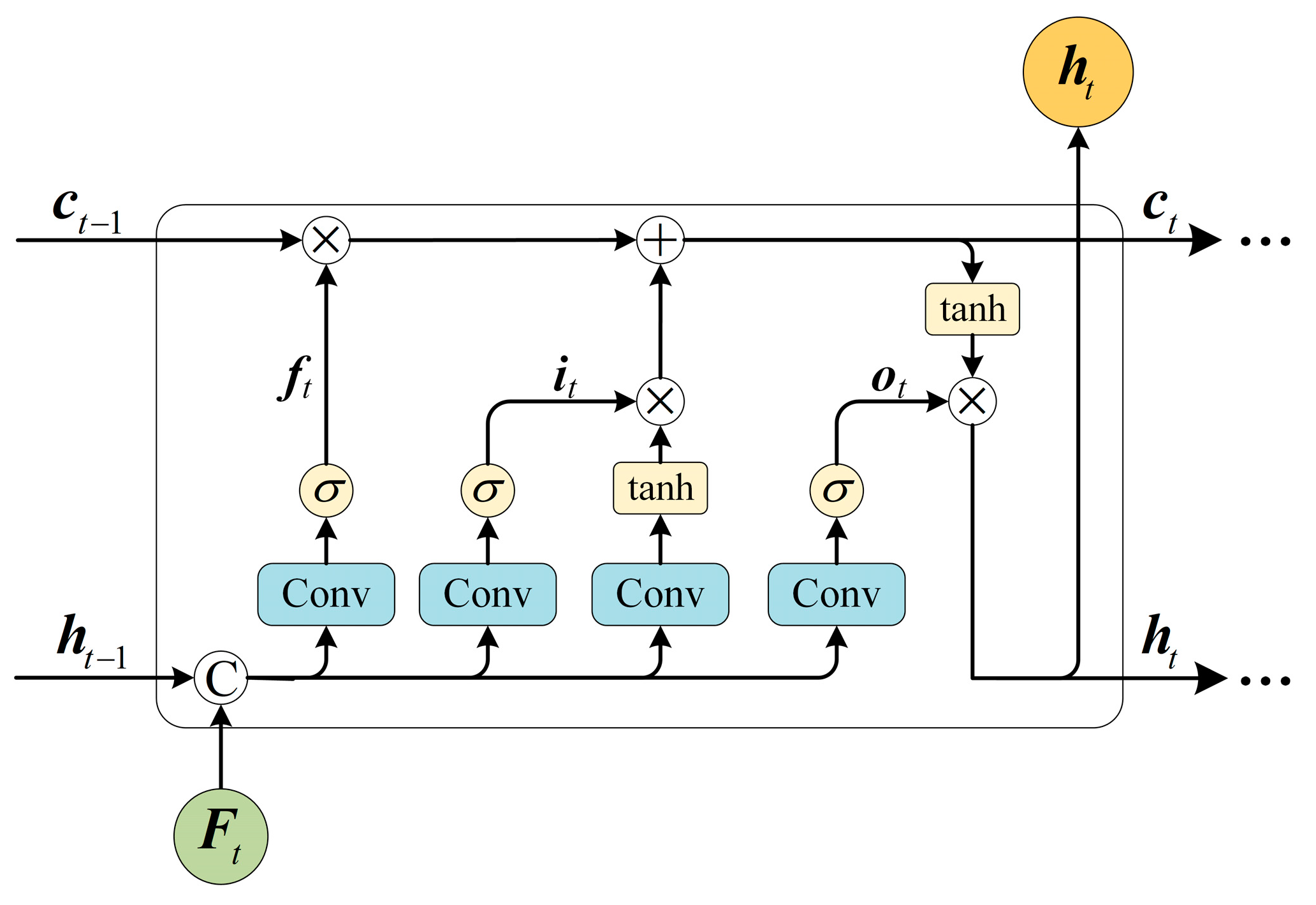
ConvLSTM can capture spatiotemporal correlations of inputs and has been widely utilized in image super-resolution, semantic segmentation, action recognition, etc. The structure of ConvLSTM is depicted in Figure 3. The ConvLSTM unit took the frame feature, F t , the previous cell, c t 1 , and the previous state, h t 1 as input, and outputted c t and h t . c t and h t represent the long-term memory and short-term memory of feature distribution, respectively. h t was further fed into the deconvolution layer for subsequent feature decoding, and finally obtained dense depth prediction results. Concretely, the ConvLSTM unit controls the storage and rewriting of feature sequence information through f t , i t , and o t . The process can be expressed as follows.
f t = σ ( W f [ F t ; F ^ t 1 ] + b f )
i t = σ ( W i [ F t ; F ^ t 1 ] + b i )
o t = σ ( W o [ F t ; F ^ t 1 ] + b o )
c t = f t c t 1 + i t tanh ( W c [ F t ; F ^ t 1 ] + b c )
F ^ t = o t tanh ( c t )
where [ ; ] denotes the concatenation operation and denotes the convolution operator. represents the element-wise product. It can be seen from the above formula that the forget gate controls where the previous memory, h t 1 , needs to be forgotten, the input gate regulates the feature to be updated, and the output gate restrains the information to be transmitted to the current state unit. To enhance the robustness of spatiotemporal information modeling, we adopted the multi-scale spatiotemporal feature modeling scheme and embedded ConvLSTM in front of each deconvolution layer in the decoding stage. This way, the proposed network could capture feature transformation with varying motion speeds and model more complementary spatiotemporal features, generating more robust spacecraft depth completion results.

3.4. Loss Functions

Similar to what is carried out for most existing depth completion networks, we utilized the mean absolute error as the loss function for S2DCNet. It should be noted that we assigned a depth of 0 to the pixels with a low foreground probability during the testing phase. Therefore, the loss function solely focuses on the depth error of pixels within the forecasted foreground by FSNet. The loss function of S2DCNet can be explicitly formulated as follows:
L = 1 N ( A ^ ) x i A ^ | d ^ ( x i ) d ( x i ) |
where A ^ signifies the set of pixels where the foreground probability surpasses the threshold t h . d ^ ( x 1 ) and d ( x i ) represent the predicted and the factual depth for pixel x i , respectively.

3.5. Dataset Construction

Deep learning-based methods demand adequate data for network weight fine-tuning, and the lack of a public dataset for video spacecraft depth completion hampers the progress of this field. To this end, we collected 126 spacecraft CAD models and constructed a large-scale dataset for training and evaluating sequential satellite depth completion algorithms. Specifically, we utilized the blender software to perform camera imaging simulation based on the different CAD models, and the built-in sun lighting model was utilized to simulate sunlight during the simulation process. The key parameters of different sensors are shown in Table 1. Based on general satellite dimensions, solar panels and body sizes were randomly assigned within the range of 3–8 m and 1–3 m, respectively. Regarding material properties, we empirically adjusted their reflectivity and roughness settings based on the components’ material categories [41] to enhance the visual realism of the simulated images.
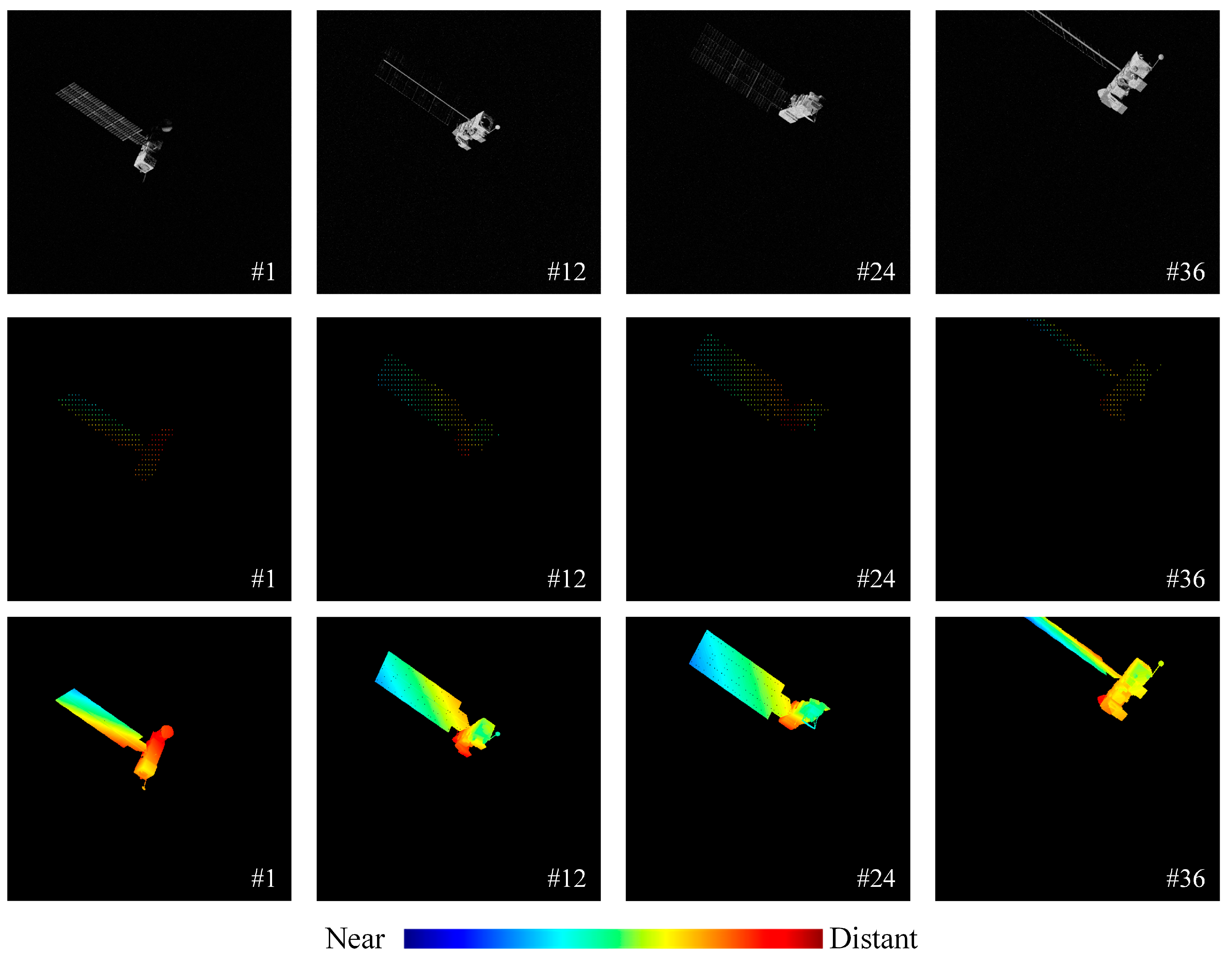
We simulated 5 sets of video sequences for each satellite model, each containing 36 frames of sensor data. Figure 4 shows the simulated video sequences. In each video, the initial pose was randomly initialized and the initial distance of the satellite relative to the sensor was within [120 m, 180 m]. The initial angle between the illumination and observation angle was in the range of 0–70°. During video simulation, the spacecraft rotated vp + ap⋅(i − 1) degrees along a specific axis at different frames (vp and a p are constants sampled from [ 2 , 10 ] and [ 0 , 1 ] , respectively. i denotes the frame index). Similarly, the spacecraft translated v l + a l ( i 1 ) meters along a particular axis ( v l and a l are constants sampled from [ 0 , 1 ] and [ 0.01 , 0.01 ] , respectively). This way, 630 satellite videos with different poses, lighting conditions, and motion patterns were generated. It is worth noting that during the simulation process, we imposed a restriction to limit the maximum angle between the optical axis and the lighting direction to 70°. This constraint resulted in our dataset lacking data under extremely unfavorable lighting conditions. Furthermore, the motion patterns of a spacecraft may be more diverse and complex in real on-orbit scenarios. These are the limitations of the constructed dataset that need improvement in future simulation work. Finally, we randomly divided the simulated video sequences into three subsets according to the used satellite CAD model: a training set (495 video sequences obtained from 99 CAD models, totaling 17,820 frames), validation set (45 video sequences obtained from 9 CAD models, totaling 1620 frames), and test set (90 video sequences obtained from 18 CAD models, totaling 3240 frames). This partitioning method ensured that validation and test models are invisible in the training phase, thus guaranteeing the algorithm’s applicability to unknown satellites.

4. Experiment Results and Discussion

4.1. Architecture Details

In terms of specific network architecture parameters, the number of channels in the encoding stage was configured as 64, 128, 256, 256, and 256, corresponding to feature maps with resolutions of 1/2, 1/4, 1/8, 1/16, and 1/32 of the original input size. The number of non-overlapping regions in the feature fusion modules at different stages was configured as 256 (M = 16). Additionally, we set the number of attention heads to four for the channel fusion layers within all feature fusion modules. In the decoding stage, the number of layers for the ConvLSTM modules was uniformly set to one, and the numbers of feature dimensions of hidden states for each module were 256, 256, 256, 128, and 64, respectively.
The detailed structural parameters of FSNet are outlined in Table 2, where the symbols k, s, and p represent the kernel size, stride, and padding size, respectively. Owing to FSNet taking the concatenation of gray image and LIDAR data as input, the number of input channels of the first convolutional layer was 2. It is also worth noting that, except for the final convolutional layer, which was followed by a Sigmoid normalization function, all convolutional and deconvolutional layers were followed by a batch normalization (BN) layer and a ReLU activation function.

4.2. Experiment Setup

We implemented the S2DCNet using the Paddle [42] library. During the training phase, the multi-stage training strategy was adopted to optimize the weight. In the first stage, with the initialization of single-frame depth completion network (SDCNet) pre-trained weights, we froze FSNet weights and fine-tuned the remaining parameters. Finally, we fine-tuned all weights in S2DCNet. Specifically, the Adam [43] optimizer was used to train the network for 50 and 25 epochs in the first and second stages, with initial learning rates of 0.001 and 0.0001, respectively. The reduce-on-plateau learning rate decay strategy was also adopted in both training stages. Furthermore, random flip and image jitter were employed to enhance network robustness. All experiments were conducted on NVIDIA Tesla V100 GPU.

4.3. Evaluation Metrics

The spacecraft depth completion task falls under the category of object-level depth completion, making traditional MAE and RMSE unsuitable as evaluation metrics for this task. To address this, Liu et al. [9] proposed four novel metrics specifically tailored for this task, which are more suitable for object-level depth completion tasks. The specific calculation formulas of these metrics are as follows:
MAEI = 1 N ( A A ^ ) x i A A ^ | d ^ ( x i ) d ( x i ) |
RMSEI = 1 N ( A A ^ ) x i A A ^ d ^ ( x i ) d ( x i ) 2 2
MATE ( α ) = 1 N ( A A ^ ) x i A A ^ min ( | d ^ ( x i ) d ( x i ) | , α )
RMSTE ( α ) = 1 N ( A A ^ ) x i A A ^ min ( d ^ ( x i ) d ( x i ) 2 2 , α 2 )
where A ^ signifies the set of pixels where the foreground probability is larger than threshold, t h . A represent the set of ground truth foreground pixels. d ^ ( x 1 ) and d ( x i ) represent the predicted and the factual depth for pixel x i , respectively. N ( A ) is the cardinality of elements within the set A . α represents the truncation threshold.
Figure 5 shows an example of one-dimensional pixel depth distribution for a better understanding of these metrics. As we all know, conventional MAE and RMSE calculate the depth error over an entire region I . However, the depth prediction error for set I A A ^ (the region correctly predicted as background) is 0, and the number of pixels in this set depends on the object’s scale. Likewise, the depth prediction error for set A A ^ A A ^ depends on the observing distance. Therefore, traditional MAE and RMSE are sensitive to the object size and observing distance, making it difficult to intuitively reflect the spacecraft depth prediction error.
To this end, MAEI, RMSEI, MATE, and RMSTE are adopted to evaluate spacecraft depth completion performance. Concretely, MAEI and RMSEI estimate the error in the set A A ^ (the area correctly predicted as foreground), and intuitively represent the foreground completion accuracy. Unlike MAEI and RMSEI, MATE and RMSTE quantify the depth prediction error within the set A A ^ . Moreover, error truncation is also performed to mitigate the undue impact of misclassified pixels on MATE and RMSTE. When the truncation threshold α is set too large (for example, larger than the distance between the spacecraft and the camera), MATE and RMSTE can be simplified as MAE, and RMSE calculated in A A ^ . In this case, MATE and RMSTE calculation results depend on an object’s distance and cannot reflect the depth prediction accuracy correctly. When α is set too small (for example, less than the depth prediction error of most pixels in area A A ^ ), the results of MATE and RMSTE are both approximately α . In this case, MATE and RMSTE also cannot correctly characterize the depth prediction accuracy. Therefore, the threshold α is generally set to a value larger than the maximum error in A A ^ and to a value smaller than the observing distance. Thus, the truncation threshold α was set to 10 m.

4.4. Results and Discussion

We compared the proposed S2DCNet with representative early fusion models (including sparse-to-dense [10], CSPN [28], DySPN [31], and PENet [32]) and late fusion models (including GuideNet [15], FCFRNet [16], RigNet [17], and SDCNet [9]). All networks were trained and evaluated on the constructed satellite video depth completion dataset, and the quantitative results are provided in Table 3. In fact, recent research [9] has shown that many existing methods are sensitive to depth sparsity and fail to obtain reasonable depth completion results with the original LIDAR data as input. Therefore, morphological preprocessing operations were adopted to obtain the optimal depth prediction results before feeding into the vanilla algorithms.
Table 3 presents the quantitative results for spacecraft depth completion using various methods. As shown in Table 3, sparse-to-dense maintains optimal computational efficiency by directly concatenating the gray images and depth maps. However, its depth completion accuracy is compromised by the challenge of fully harnessing the complementary information in multimodal data. SPN-based methods (CSPN, PENet, and DySPN) exhibit a certain level of performance enhancement over that of the early fusion model, but also increase the amount of computation. Compared with SPN-based methods, the recently proposed late fusion model exhibits promising performance and computational efficiency. Notably, SDCNet achieves the best spacecraft depth completion performance among those of existing methods while maintaining high computational efficiency. In comparison to prevailing methods for depth completion, the proposed S2DCNet utilizes ConvLSTM to exploit temporal–spatial coherence in sequential frames and outperforms existing methods across various evaluation criteria while maintaining a high inference speed and computational efficiency. Specifically, the S2DCNet processes images of size of 512 × 512 in just 42.87 milliseconds on Tesla V100 GPU. Compared to the SDCNet, the S2DCNet achieves a reduction of 16% in MAEI and of 12% in MATE while only adding an extra processing time of 6.5 milliseconds. This implies that the proposed S2DCNet is well-suited for real-time or near-real-time systems.
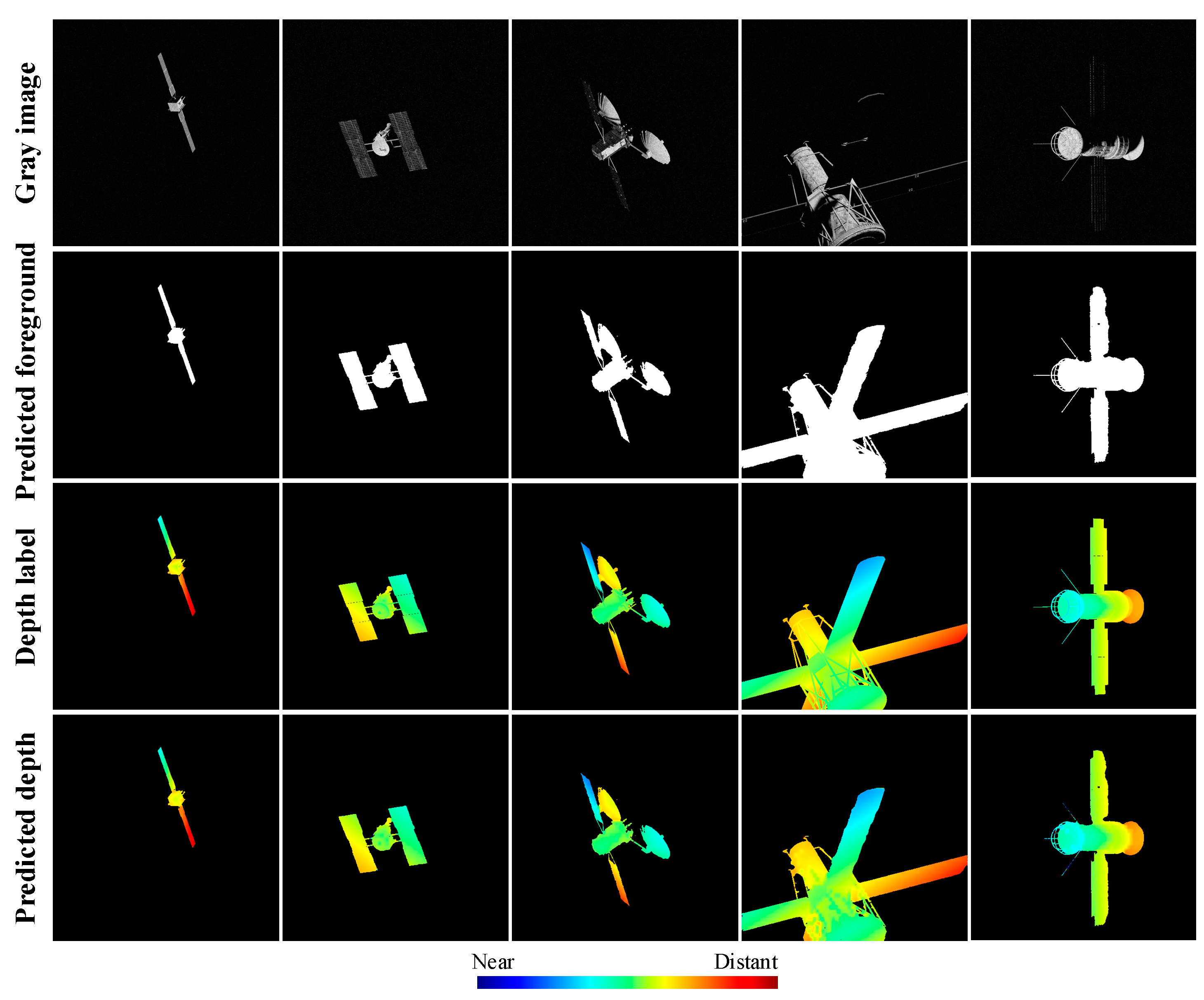
Figure 6 shows the visualization results of different spacecraft models, including gray images, foreground segmentation outcomes, depth labels, and final predicted depth maps from top to bottom. It can be seen that thanks to the sparse-ranging information supplied by LIDAR, FSNet can accurately distinguish the foreground and background. According to statistics, the intersection over union (IoU) between the predicted and the ground truth foreground region is 95.06%. Furthermore, the ultimate depth prediction results also exhibit visually gratifying quality compared to that of the depth map labels.
To qualitatively compare the performance of state-of-the-art algorithms, Figure 7 displays the prediction results and associated error maps for DySPN [31], SDCNet [9], and S2DCNet. A careful examination of the depth error map reveals that compared to those predicted by the SCNet and S2DCNet, the depth maps predicted by the DySPN exhibit notable depth errors within the spacecraft’s body region (shown in the magnified blue boxes). Additionally, it can be seen that the depth errors predicted by the SDCNet and S2DCNet are primarily concentrated around the spacecraft’s peripheral areas. As observed in the zoomed-in region highlighted by the red box in Figure 7, compared to those predicted by the SDCNet, the depth maps predicted by the S2DCNet can preserve sharper edges and richer detailed information, which is crucial for various downstream tasks (such as 3D component recognition, pose estimation, etc.).
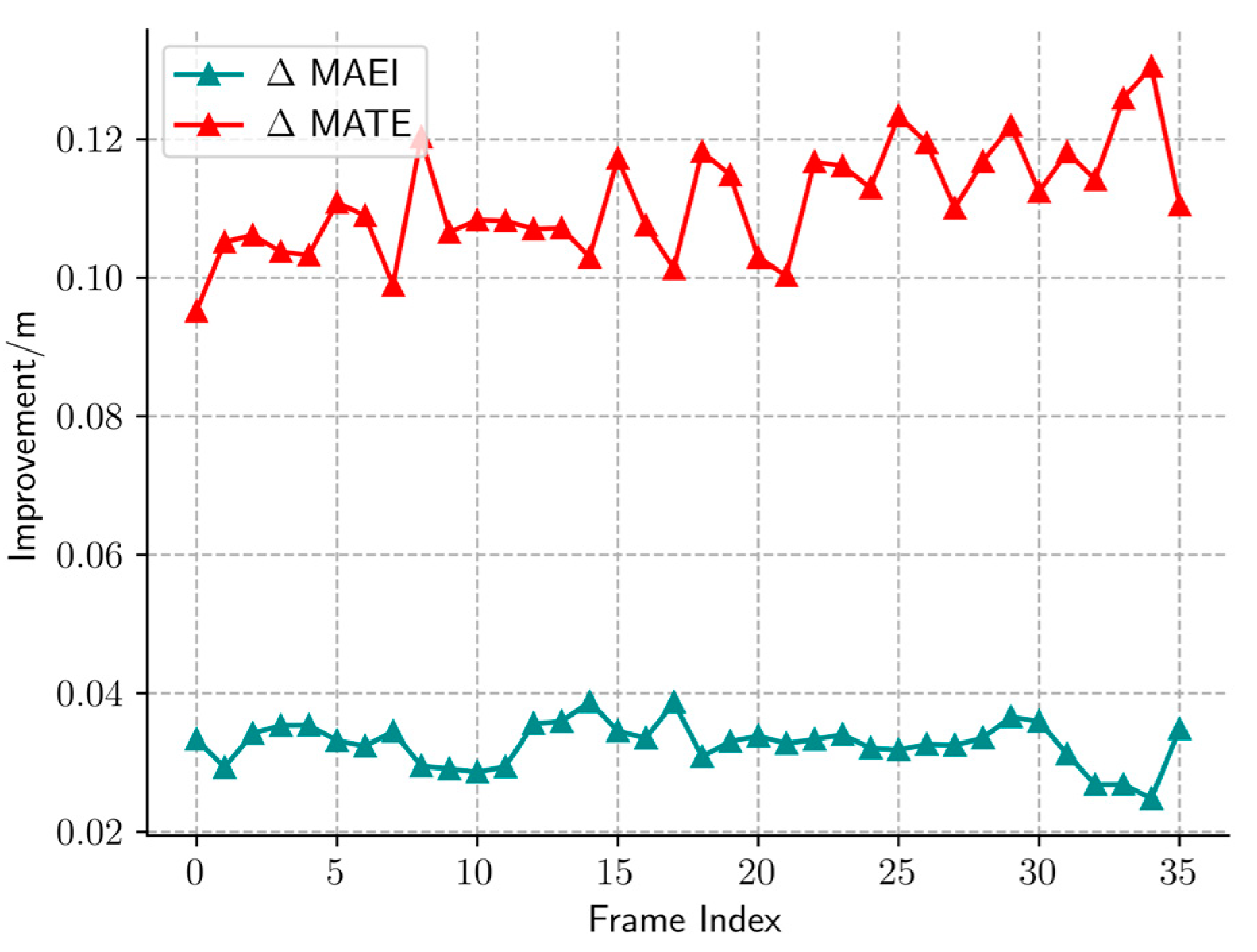
The average MAEI and MATE improvements of the S2DCNet relative to those of the SDCNet for each frame are also depicted in Figure 8, providing a quantitative assessment of the temporal evolution in prediction accuracy improvement. It can be seen that the improvement in MAEI is relatively stable, while the improvement in MATE shows an upward trend with the frame index increase.

4.5. Ablation Studies

We performed ablation studies to analyze how spatiotemporal feature modeling at various stages affects network performance. Specifically, we compared different spatiotemporal feature modeling options:
  • ConvLSTM utilizes the encoder-generated feature map as input, with its output contributing to subsequent feature decoding (referred to as E-SS modeling).
  • ConvLSTM modules are incorporated into the encoding stage with the multi-scale scheme (referred to as E-MS modeling).
  • ConvLSTM modules are incorporated into the decoding stage with the multi-scale scheme (referred to as D-MS modeling).
The quantitative results with different spatiotemporal feature modeling versions are presented in Table 4.
As shown in Table 4, the single-scale spatiotemporal modeling structure can slightly improve network performance compared to that at the baseline (SDCNet). Moreover, both “E-MS Modeling” and “D-MS Modeling” outperform the single-scale structure, verifying the effectiveness of the multi-scale spatiotemporal modeling scheme. Finally, since “D-MS Modeling” can exploit the feature correlation across frames without affecting the feature extraction of the current frame, “D-MS Modeling” performs a little bit better than “E-MS Modeling” does and achieves optimal performance. We also visualize the feature map before and after feeding into the ConvLSTM module in Figure 9. It can be seen that the feature map output by the ConvLSTM module contains richer details and sharper edges than does the original feature map. This phenomenon demonstrates that spatiotemporal feature modeling can enrich feature information and improve depth completion accuracy.

5. Conclusions

Perceiving a spacecraft’s three-dimensional structure and obtaining its point cloud data is a prerequisite for diverse on-orbit tasks, such as debris removal, on-orbit maintenance, rendezvous and docking, etc. Currently, utilizing visible light images in conjunction with LIDAR data is an effective method to obtain a spacecraft’s three-dimensional point cloud data. However, existing methods ignore inter-frame correlation information and fail to capture the temporal coherence of consecutive frames, resulting in inaccurate and temporally inconsistent depth completion results. This paper proposes a video depth completion framework named the S2DCNet to solve this problem. Specifically, in the encoding stage, the feature fusion modules, which infer channel similarity maps and spatial significance maps sequentially, were adopted to hierarchically aggregate complementary information in multimodal data. Moreover, ConvLSTM modules were incorporated into the decoding stage with the multi-scale scheme to explore temporal–spatial feature correlations, generating more accurate and temporally consistent depth results through perceiving past feature states. Finally, a satellite video depth completion dataset was constructed which contains 630 satellite videos (totaling 22,680 frames) with different poses, lighting conditions, and motion patterns. Empirical experiments on the dataset substantiated the efficacy of the proposed approach. The experiments underscored the outstanding performance of the proposed S2DCNet, with an achieved MAEI and MATE of 0.192 m and 0.645 m, respectively. Considering the accuracy and efficiency of the S2DCNet, the S2DCNet holds the promise of seamless integration into spacecraft on-orbit perception systems.

Author Contributions

Investigation, literature analysis, methodology, writing—original draft, and validation, X.L.; satellite collection, H.W.; project administration, supervision, and revising and editing, X.C. and W.C.; data simulation, Z.X. All authors have read and agreed to the published version of the manuscript.

Funding

This research received no external funding.

Institutional Review Board Statement

Not applicable.

Informed Consent Statement

Not applicable.

Data Availability Statement

Part of the data presented in this paper are available at https://drive.google.com/file/d/1-zZdc_Ar3p3RFXyUim6czRX2_lgWOM-r/view?usp=drive_link (accessed on 14 September 2023). After completing subsequent projects, additional data may be made accessible upon reasonable requests for academic research purposes.

Conflicts of Interest

The authors declare no conflict of interest.

References

  1. Santos, R.; Rade, D.; Fonseca, D. A machine learning strategy for optimal path planning of space robotic manipulator in on-orbit servicing. Acta Astronaut. 2022, 191, 41–54. [Google Scholar] [CrossRef]
  2. Henshaw, C. The darpa phoenix spacecraft servicing program: Overview and plans for risk reduction. In Proceedings of the International Symposium on Artificial Intelligence, Robotics and Automation in Space (I-SAIRAS), Montreal, QC, Canada, 17–19 June 2014. [Google Scholar]
  3. Liu, Y.; Xie, Z.; Liu, H. Three-line structured light vision system for non-cooperative satellites in proximity operations. Chin. J. Aeronaut. 2020, 33, 1494–1504. [Google Scholar] [CrossRef]
  4. Guo, J.; He, Y.; Qi, X.; Wu, G.; Hu, Y.; Li, B.; Zhang, J. Real-time measurement and estimation of the 3D geometry and motion parameters for spatially unknown moving targets. Aerosp. Sci. Technol. 2020, 97, 105619. [Google Scholar] [CrossRef]
  5. Liu, X.; Wang, H.; Chen, X.; Chen, W.; Xie, Z. Position Awareness Network for Noncooperative Spacecraft Pose Estimation Based on Point Cloud. IEEE Trans. Aerosp. Electron. Syst. 2022, 59, 507–518. [Google Scholar] [CrossRef]
  6. Wei, Q.; Jiang, Z.; Zhang, H. Robust spacecraft component detection in point clouds. Sensors 2018, 18, 933. [Google Scholar] [CrossRef] [PubMed]
  7. De, J.; Jordaan, H.; Van, D. Experiment for pose estimation of uncooperative space debris using stereo vision. Acta Astronaut. 2020, 168, 164–173. [Google Scholar]
  8. Jacopo, V.; Andreas, F.; Ulrich, W. Pose tracking of a noncooperative spacecraft during docking maneuvers using a time-of-flight sensor. In Proceedings of the AIAA Guidance, Navigation, and Control Conference (GNC), San Diego, CA, USA, 4–8 January 2016. [Google Scholar]
  9. Liu, X.; Wang, H.; Yan, Z.; Chen, Y.; Chen, X.; Chen, W. Spacecraft depth completion based on the gray image and the sparse depth map. IEEE Trans. Aerosp. Electron. Syst. 2023, in press. [CrossRef]
  10. Ma, F.; Karaman, S. Sparse-to-dense: Depth prediction from sparse depth samples and a single image. In Proceedings of the International Conference on Robotics and Automation (ICRA), Brisbane, QLD, Australia, 21–25 May 2018. [Google Scholar]
  11. Imran, S.; Long, Y.; Liu, X.; Morris, D. Depth coefficients for depth completion. In Proceedings of the Conference on Computer Vision and Pattern Recognition (CVPR), Long Beach, CA, USA, 15–20 June 2019. [Google Scholar]
  12. Teixeira, L.; Oswald, M.; Pollefeys, M.; Chli, M. Aerial single-view depth completion with image-guided uncertainty estimation. IEEE Robots. Autom. Lett. 2020, 5, 1055–1062. [Google Scholar] [CrossRef]
  13. Luo, Z.; Zhang, F.; Fu, G.; Xu, J. Self-Guided Instance-Aware Network for Depth Completion and Enhancement. In Proceedings of the International Conference on Robotics and Automation (ICRA), Xi’an, China, 30 May–5 June 2021. [Google Scholar]
  14. Chen, Y.; Yang, B.; Liang, M.; Urtasun, R. Learning joint 2d-3d representations for depth completion. In Proceedings of the International Conference on Computer Vision (ICCV), Seoul, Korea, 27 October–2 November 2019. [Google Scholar]
  15. Tang, J.; Tian, F.; Feng, W.; Li, J.; Tan, P. Learning guided convolutional network for depth completion. IEEE Trans. Image Process. 2020, 30, 1116–1129. [Google Scholar] [CrossRef] [PubMed]
  16. Liu, L.; Song, X.; Lyu, X.; Diao, J.; Wang, M.; Liu, Y.; Zhang, L. Fcfr-net: Feature fusion based coarse-to-fine residual learning for depth completion. In Proceedings of the AAAI Conference on Artificial Intelligence (AAAI), Vancouver, BC, Canada, 2–9 February 2021. [Google Scholar]
  17. Yan, Z.; Wang, K.; Li, X.; Zhang, Z.; Xu, B.; Li, J.; Yang, J. RigNet: Repetitive image guided network for depth completion. In Proceedings of the European Conference on Computer Vision (ECCV), Tel Aviv, Israel, 23–27 October 2022. [Google Scholar]
  18. Giang, K.; Song, S.; Kim, D.; Choi, S. Sequential Depth Completion with Confidence Estimation for 3D Model Reconstruction. IEEE Robots. Autom. Lett. 2020, 6, 327–334. [Google Scholar] [CrossRef]
  19. Nguyen, T.; Yoo, M. Dense-depth-net: A spatial-temporal approach on depth completion task. In Proceedings of the Region 10 Symposium (TENSYMP), Jeju, Korea, 23–25 August 2021. [Google Scholar]
  20. Chen, Y.; Zhao, S.; Ji, W.; Gong, M.; Xie, L. MetaComp: Learning to Adapt for Online Depth Completion. arXiv 2022, arXiv:2207.10623. [Google Scholar]
  21. Yang, Q.; Yang, R.; Davis, J.; Nister, D. Spatial-depth super resolution for range images. In Proceedings of the Conference on Computer Vision and Pattern Recognition (CVPR), Minneapolis, MN, USA, 17–22 June 2007. [Google Scholar]
  22. Kopf, J.; Cohen, M.; Lischinski, D.; Uyttendaele, M. Joint bilateral upsampling. ACM Trans. Graph. 2007, 26, 96–101. [Google Scholar] [CrossRef]
  23. Ferstl, D.; Reinbacher, C.; Ranftl, R.; Ruther, M.; Bischof, H. Image guided depth upsampling using anisotropic total generalized variation. In Proceedings of the International Conference on Computer Vision (ICCV), Sydney, NSW, Australia, 1–8 December 2013. [Google Scholar]
  24. Barron, J.; Poole, B. The fast bilateral solver. In Proceedings of the European Conference on Computer Vision (ECCV), Amsterdam, The Netherlands, 8–16 October 2016. [Google Scholar]
  25. He, K.; Sun, J.; Tang, X. Guided image filtering. IEEE Trans Pattern Anal. Mach. Intell. 2012, 35, 1397–1409. [Google Scholar] [CrossRef] [PubMed]
  26. Lee, H.; Soohwan, S.; Sungho, J. 3D reconstruction using a sparse laser scanner and a single camera for outdoor autonomous vehicle. In Proceedings of the International Conference on Intelligent Transportation Systems (ITSC), Rio de Janeiro, Brazil, 1–4 November 2016. [Google Scholar]
  27. Liu, S.; Mello, D.; Gu, J.; Zhong, G.; Yang, M.; Kautz, J. Learning affinity via spatial propagation networks. In Proceedings of the Advances in Neural Information Processing Systems, Long Beach, CA, USA, 4–9 December 2017. [Google Scholar]
  28. Cheng, X.; Wang, P.; Yang, R. Learning depth with convolutional spatial propagation network. IEEE Trans Pattern Anal. Mach. Intell. 2019, 42, 2361–2379. [Google Scholar] [CrossRef] [PubMed]
  29. Cheng, X.; Wang, P.; Guan, C.; Yang, R. Cspn++: Learning context and resource aware convolutional spatial propagation networks for depth completion. In Proceedings of the AAAI Conference on Artificial Intelligence (AAAI), New York, NY, USA, 7–12 February 2020. [Google Scholar]
  30. Park, J.; Joo, K.; Hu, Z.; Liu, C.; So, K. Non-local spatial propagation network for depth completion. In Proceedings of the European Conference on Computer Vision (ECCV), Glasgow, Scotland, UK, 23–28 August 2020. [Google Scholar]
  31. Lin, Y.; Cheng, T.; Zhong, Q.; Zhou, W.; Yang, H. Dynamic spatial propagation network for depth completion. In Proceedings of the AAAI Conference on Artificial Intelligence (AAAI), Virtual, 22 February–1 March 2022. [Google Scholar]
  32. Hu, M.; Wang, S.; Li, B.; Ning, S.; Fan, L.; Gong, X. Penet: Towards precise and efficient image guided depth completion. In Proceedings of the International Conference on Robotics and Automation (ICRA), Xi’an, China, 30 May–5 June 2021. [Google Scholar]
  33. Li, Y.; Xu, Q.; Li, W.; Nie, J. Automatic clustering-based two-branch CNN for hyperspectral image classification. IEEE Trans. Geosci. Remote Sens. 2020, 59, 7803–7816. [Google Scholar] [CrossRef]
  34. Yang, J.; Zhao, Y.; Chan, J. Hyperspectral and multispectral image fusion via deep two-branches convolutional neural network. Remote Sens. 2018, 10, 800. [Google Scholar] [CrossRef]
  35. Fu, Y.; Wu, X. A dual-branch network for infrared and visible image fusion. In Proceedings of the International Conference on Pattern Recognition (ICPR), Milan, Italy, 10–15 January 2021. [Google Scholar]
  36. Li, Y.; Xu, Q.; He, Z.; Li, W. Progressive Task-based Universal Network for Raw Infrared Remote Sensing Imagery Ship Detection. IEEE Trans. Geosci. Remote Sens. 2023, 61, 1–13. [Google Scholar] [CrossRef]
  37. Ku, J.; Harakeh, A.; Waslander, S. In defense of classical image processing: Fast depth completion on the CPU. In Proceedings of the Conference on Computer and Robot Vision (CRV), Toronto, ON, Canada, 8–10 May 2018. [Google Scholar]
  38. Uhrig, J.; Schneider, N.; Schneider, L.; Franke, U.; Brox, T.; Geiger, A. Sparsity invariant CNNs. In Proceedings of the International Conference on 3D Vision (3DV), Qingdao, China, 10–12 October 2017. [Google Scholar]
  39. Vaswani, A.; Shazeer, N.; Parmar, N.; Uszkoreit, J.; Jones, L.; Gomez, A.; Kaiser, L.; Polosukhin, I. Attention is all you need. In Proceedings of the Advances in Neural Information Processing Systems, Long Beach, CA, USA, 4–9 December 2017. [Google Scholar]
  40. Shi, X.; Chen, Z.; Wang, H.; Yeung, D.; Wong, W.; Woo, W. Convolutional LSTM network: A machine learning approach for precipitation nowcasting. In Proceedings of the Advances in Neural Information Processing Systems, Montreal, QC, Canada, 7–12 December 2015. [Google Scholar]
  41. Wang, H.; Ning, Q.; Yan, Z.; Liu, X.; Lu, Y. Research on elaborate image simulation method for close-range space target. J. Mod. Opt. 2023, 70, 205–216. [Google Scholar] [CrossRef]
  42. Ma, Y.; Yu, D.; Wu, T.; Wang, H. PaddlePaddle: An open-source deep learning platform from industrial practice. Front. Data Comput. 2019, 1, 105–115. [Google Scholar]
  43. Kingma, D.; Ba, J. Adam: A method for stochastic optimization. In Proceedings of the International Conference on Learning Representations, San Diego, CA, USA, 7–9 May 2015. [Google Scholar]
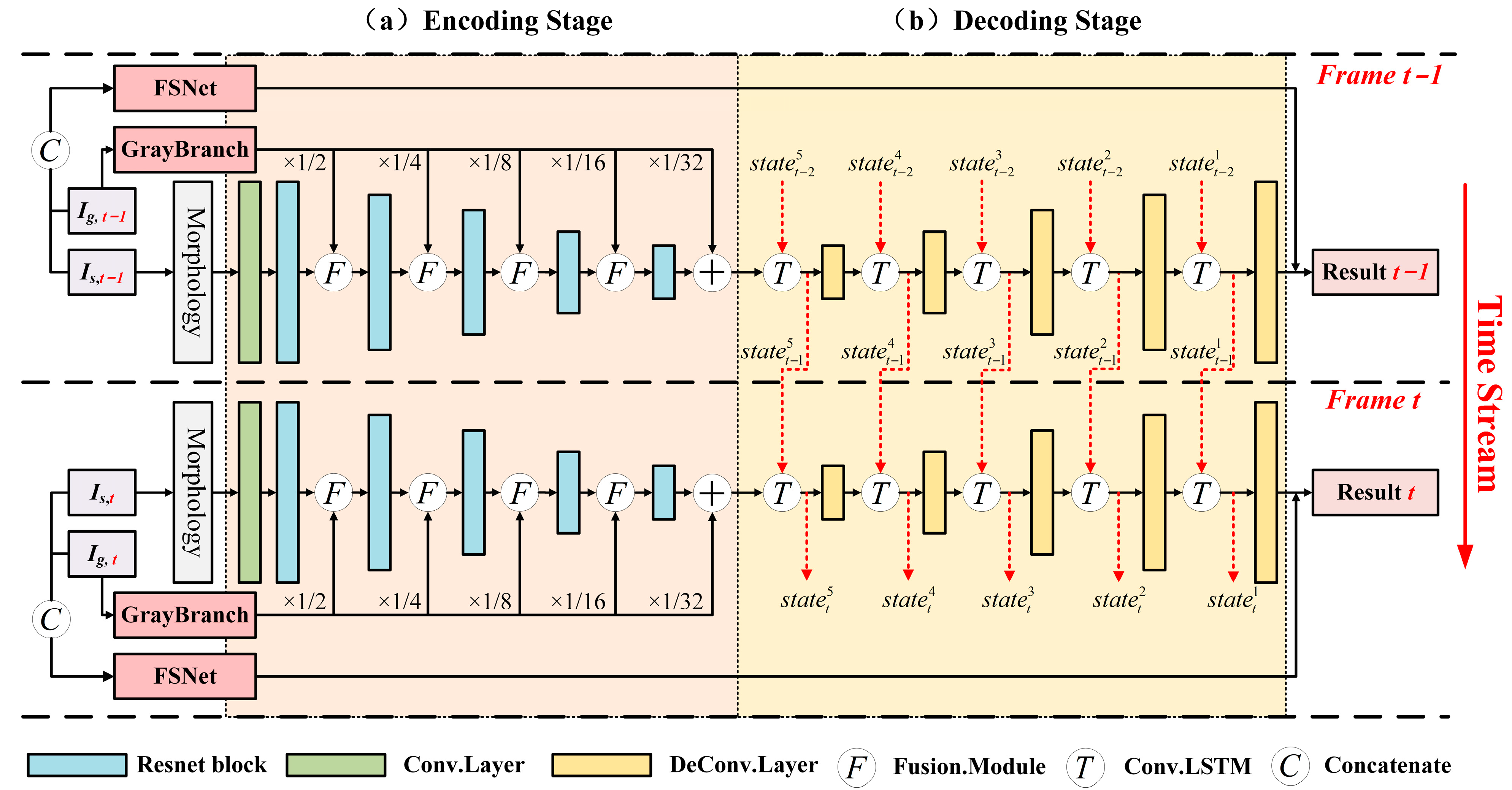
Figure 1. Overview of sequential spacecraft depth completion network (S2DCNet). (a) and (b) represent the encoding stage and decoding stage, respectively. S2DCNet utilized the feature fusion module to aggregate the semantic and depth information in multimodal data in the encoding stage and captured spatiotemporal feature correlations across frames through ConvLSTM modules in the decoding stage. Moreover, the FSNet was adopted to segment the foreground and compute the foreground pixels’ depth regression loss. Arrows represent the direction of data flow.
Remotesensing 15 04786 g001
Figure 2. The configuration of the feature fusion module, predominantly comprising the embedding layer, channel fusion layer, and spatial fusion layer. (a) Illustration of the overall structure of the feature fusion module. (bd) Illustration of the detailed structures for the embedding layer, channel fusion layer, and spatial fusion layer, respectively.
Remotesensing 15 04786 g002
Figure 3. The ConvLSTM unit is structured with distinct components: a forget gate denoted as f t , an input gate represented by i t , and an output gate indicated by o t . This unit takes the feature F t , along with the memory cell, c t 1 , and the hidden state, h t 1 , at time t − 1 as input. It then produces c t and h t . The hidden state, h t , is further used for subsequent feature decoding.
Remotesensing 15 04786 g003
Figure 4. An example of simulated video sequences with the gray image, sparse depth (LIDAR data) and actual depth map, arranged from top to bottom. The number in the bottom right corner of the image represents the frame index.
Remotesensing 15 04786 g004
Figure 5. An example of 1D pixel depth prediction distribution. Districts A , A ^ , and I denote the ground truth foreground area, the predicted foreground area, and the entire image area, respectively.
Remotesensing 15 04786 g005
Figure 6. The visualization results of the proposed S2DCNet, showcasing gray images, foreground segmentation outcomes, depth labels, and final predicted depth maps from top to bottom.
Remotesensing 15 04786 g006
Figure 7. Qualitative comparison of the DySPN [31], SDCNet [9], and proposed S2DCNet. Pseudo-colored predictions and pseudo-colored error maps are provided for easier comparison. It is noted that the background in predicted depth maps is set to black for better visualization.
Remotesensing 15 04786 g007
Figure 8. The average MAEI and MATE improvements of the S2DCNet relative to those of the SDCNet for each frame in the test set.
Remotesensing 15 04786 g008
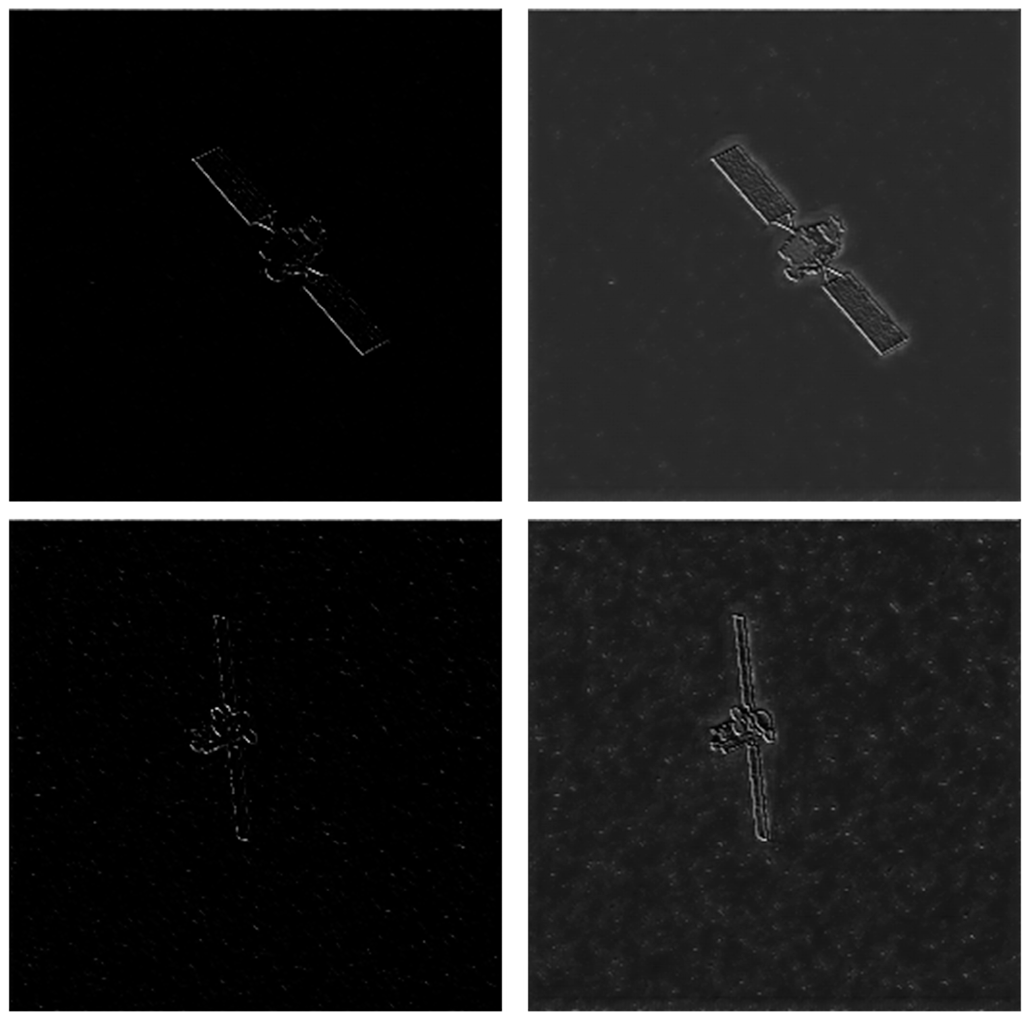
Figure 9. The visualization of the original feature map and the enhanced feature map, arranged from left to right.
Remotesensing 15 04786 g009
Table 1. The sensor parameters of the optical camera and LIDAR.
Sensor TypeSensor ParameterValue
optical camerafocal length50 mm
field of view7.38° × 7.38°
sensor size6.449 mm × 6.449 mm
color typemonochrome
image size512 pixel × 512 pixel
LIDARrange2–280 m
horizontal angle resolution0.09°
vertical angle resolution0.13°
accuracy (1σ)30 mm
Table 2. The detailed parameters of each layer of the foreground segmentation network (FSNet). The parameters k, s, and p represent the kernel size, stride, and padding size.
Layer IndexLayer TypeLayer Parameter/
(k, s, p)
Input ChannelOut Channel
1Convolution(5, 1, 2)216
2Convolution(3, 2, 1)1616
3Convolution(3, 2, 1)1632
4Convolution(3, 2, 1)3264
5Deconvolution(3, 2, 1)6432
6Deconvolution(3, 2, 1)3216
7Deconvolution(3, 2, 1)1616
8Convolution(3, 1, 1)161
Table 3. The completion accuracy of diverse methods. The methods with * take the depth map derived from morphological preprocessing as input.
MethodsMAEI/mMATE/mRMSEI/mRMSTE/mInference Time/ms
Sparse-to-dense * [10]2.0993.6132.9005.0126.93
CSPN [28]1.3122.1591.9993.55847.26
PENet * [32]0.2601.0850.7272.92796.72
DySPN * [31]0.4520.8050.7352.30445.48
GuideNet * [15]0.3950.8811.0682.38039.46
FCFRNet * [16]0.8211.3861.5332.79987.55
RigNet * [17]0.2991.5290.8713.52553.95
SDCNet [9]0.2290.7350.6112.26636.33
S2DCNet (ours)0.1920.6450.5112.10642.87
Table 4. The quantitative results of different spatiotemporal feature modeling structures.
VersionsMAEI/mMATE/mRMSEI/mRMSTE/m
baseline0.2290.7350.6112.266
E-SS modeling0.2090.7040.5642.209
E-MS modeling0.1990.6870.5472.186
D-MS modeling0.1920.6450.5112.106
Disclaimer/Publisher’s Note: The statements, opinions and data contained in all publications are solely those of the individual author(s) and contributor(s) and not of MDPI and/or the editor(s). MDPI and/or the editor(s) disclaim responsibility for any injury to people or property resulting from any ideas, methods, instructions or products referred to in the content.