Article

Small-Sample Underwater Target Detection: A Joint Approach Utilizing Diffusion and YOLOv7 Model

School of Marine Science and Technology, Northwestern Polytenical University, Xi’an 710072, China
*
Author to whom correspondence should be addressed.
Remote Sens. 2023, 15(19), 4772; https://doi.org/10.3390/rs15194772
Submission received: 2 August 2023 / Revised: 25 September 2023 / Accepted: 27 September 2023 / Published: 29 September 2023
(This article belongs to the Special Issue Advancement in Undersea Remote Sensing)

Abstract

:
Underwater target detection technology plays a crucial role in the autonomous exploration of underwater vehicles. In recent years, significant progress has been made in the field of target detection through the application of artificial intelligence technology. Effectively applying AI techniques to underwater target detection is a highly promising area of research. However, the difficulty and high cost of underwater acoustic data collection have led to a severe lack of data, greatly restricting the development of deep-learning-based target detection methods. The present study is the first to utilize diffusion models for generating underwater acoustic data, thereby effectively addressing the issue of poor detection performance arising from the scarcity of underwater acoustic data. Firstly, we place iron cylinders and cones underwater (simulating small preset targets such as mines). Subsequently, we employ an autonomous underwater vehicle (AUV) equipped with side-scan sonar (SSS) to obtain underwater target data. The collected target data are augmented using the denoising diffusion probabilistic model (DDPM). Finally, the augmented data are used to train an improved YOLOv7 model, and its detection performance is evaluated on a test set. The results demonstrate the effectiveness of the proposed method in generating similar data and overcoming the challenge of limited training sample data. Compared to models trained solely on the original data, the model trained with augmented data shows a mean average precision (mAP) improvement of approximately 30% across various mainstream detection networks. Additionally, compared to the original model, the improved YOLOv7 model proposed in this study exhibits a 2% increase in mAP on the underwater dataset.

1. Introduction

In autonomous exploration tasks of AUVs, target detection technology based on SSS imagery plays a crucial role [1,2,3]. Among traditional detection methods and deep-learning-based detection methods, deep-learning-based approaches have shown significant advantages and have seen extensive applications in the field of underwater target detection [4,5,6]. However, the quantity and quality of data samples directly impact the detection performance of deep learning methods. Obtaining sufficient high-quality target data is extremely challenging and costly due to an AUV’s unstable underwater posture and positioning errors caused by cumulative inaccuracies. Therefore, it is of paramount significance for research to explore how to generate data from small-sample SSS images and improve target detection performance.
In terms of data generation, deep generative models, such as VAE [7,8], EBM [9,10], GANs [11,12,13], normalizing flow [14,15], and diffusion model [16,17], have shown great potential in creating new patterns that humans cannot properly distinguish. However, due to the unique characteristics of underwater data, there is relatively limited research on data augmentation specifically for underwater data. Current research generally relies on the combination of some simulation models and GANs for data generation.
If only a set of original data is available, conditional GANs and some unconditional GANs can be considered. By providing either target images or target images with labels as input, GANs can fit simulated images to approach real images through random noise. Chen et al. [18] proposed a deep convolutional generative adversarial network (SGAN) based on group padding and uniform-sized convolutional kernels, which is used for high-quality data augmentation. Xu et al. [19] combined DenseNet and ResNet with WGAN-GP to propose an image generation network called CWGAN-GP&DR, which extends underwater sonar datasets and effectively improves the classification performance of underwater sonar images. Wang et al. [20] addressed the issues of low resolution and poor imaging quality in commonly used image generation methods. They proposed a new model based on DCGAN, improving the network structure and the loss function of the discriminator. They also introduced a controllable multi-layer transformed convolutional layer structure, enhancing the image resolution and imaging quality.
If pixel-level paired training images are available, GANs based on pix2pix can be used to generate images. Jegorova et al. [21] proposed a novel method for generating realistic SSS images called Markov-chain-conditioned pix2pix (MC-pix2pix) and used MC-pix2pix data to train an autonomous target detection network. Jiang et al. [22] presented a pix2pix-based semantic image synthesis model. The proposed method reconstructs SSS-simulated images from simple hand-drawn segmentation maps of target photos and can generate sonar images with different water depths and frequencies. Lee et al. [23] used a segmentation network to obtain mask images from the original images for training the pix2pix network. The trained network is then used to generate sonar images to enhance the effectiveness of the segmentation network.
In addition to single-group image data and paired image data, unsupervised GAN networks like CycleGAN can also be utilized. CycleGAN takes two sets of unlabeled data as input and employs a method similar to style transfer to achieve target data generation. Liu et al. [24] developed a novel humanized underwater acoustic image simulator based on 3D modeling software. Then, using the dataset generated by the simulator, they applied the CycleGAN network to generate realistic acoustic images. Zhang et al. [25] addressed the issue of imbalanced and speckle-noise-prone acoustic images that often lead to mode collapse. They proposed a spectrum normalization CycleGAN network, where spectrum normalization is applied to both the generator and discriminator to stabilize GAN training.
The aforementioned data generation methods based on GANs require a relatively large dataset for training, and GAN training can be challenging. When the dataset is small, it can easily lead to mode collapse, necessitating certain complex techniques to improve the training process [26]. On the other hand, diffusion models, compared to GANs, are more stable and do not require an additional discriminator to be trained. Therefore, diffusion models have shown great potential in various fields, such as computer vision [27,28], sequence modeling [29,30], audio processing [31,32], and artificial intelligence research [33,34]. However, there is currently no research on diffusion models specifically for generating underwater SSS data.
The diffusion model has achieved success in many fields, making it highly worthwhile to explore how to apply the diffusion model to one’s own research domain. This paper utilizes a small-sample dataset of SSS data collected from sea trials to train a diffusion model and compares it with generation methods based on GANs. The effectiveness of the diffusion model in generating small-sample SSS data is demonstrated. Finally, the generated data are tested on mainstream detection networks and an improved YOLOv7 network to further validate the enhancement in detection accuracy achieved by training networks with data generated by the diffusion model.
The contributions of this paper can be summarized as follows:
(1)
The first application of the DDPM to generate small-sample SSS data yielded excellent results in the experiments. It addresses the challenges associated with acquiring SSS data using an AUV and reduces data collection costs.
(2)
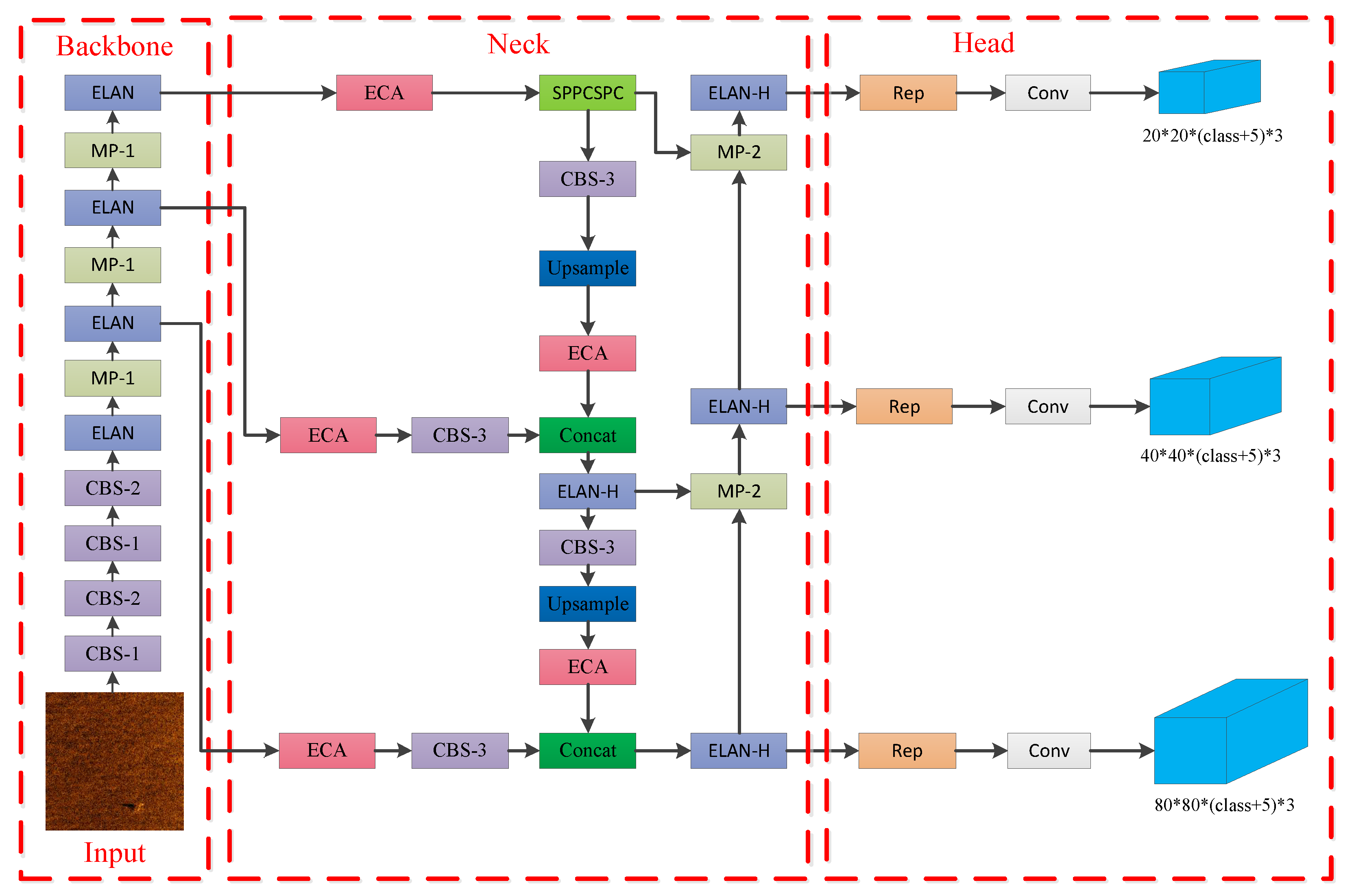
An improvement was made to the YOLOv7 model by introducing an ECANet attention mechanism to the YOLOv7 network, enhancing the feature extraction capability for underwater targets and improving the detection accuracy of small targets in SSS images.
(3)
A dataset of small underwater targets in SSS was constructed, and a comprehensive comparison was conducted between current mainstream data generation methods and object detection methods on this dataset, fully demonstrating the effectiveness of the proposed approach in this paper.
The rest of this paper is organized as follows: In Section 2, we introduce the diffusion-model-based data generation method and the improved YOLOv7 network structure used in this study. Section 3 presents the experimental process and showcases the results. In Section 4, we discuss the strengths and limitations of the proposed methods. Section 5 concludes the paper and provides an outlook on future work.

2. Methods

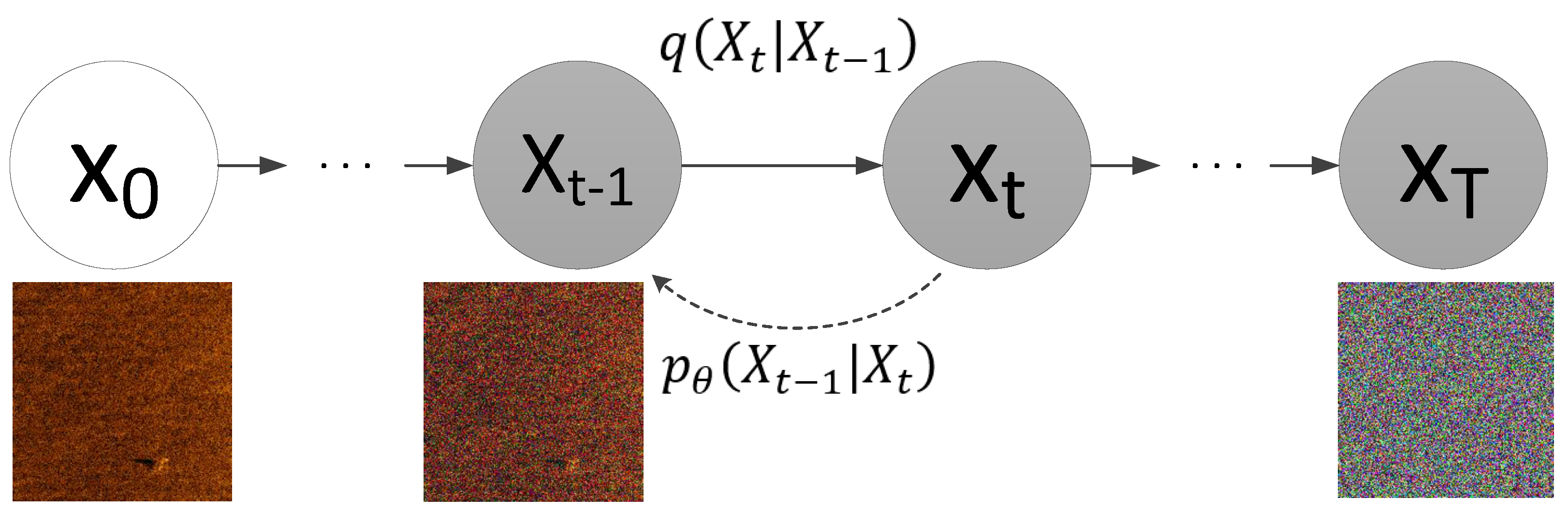
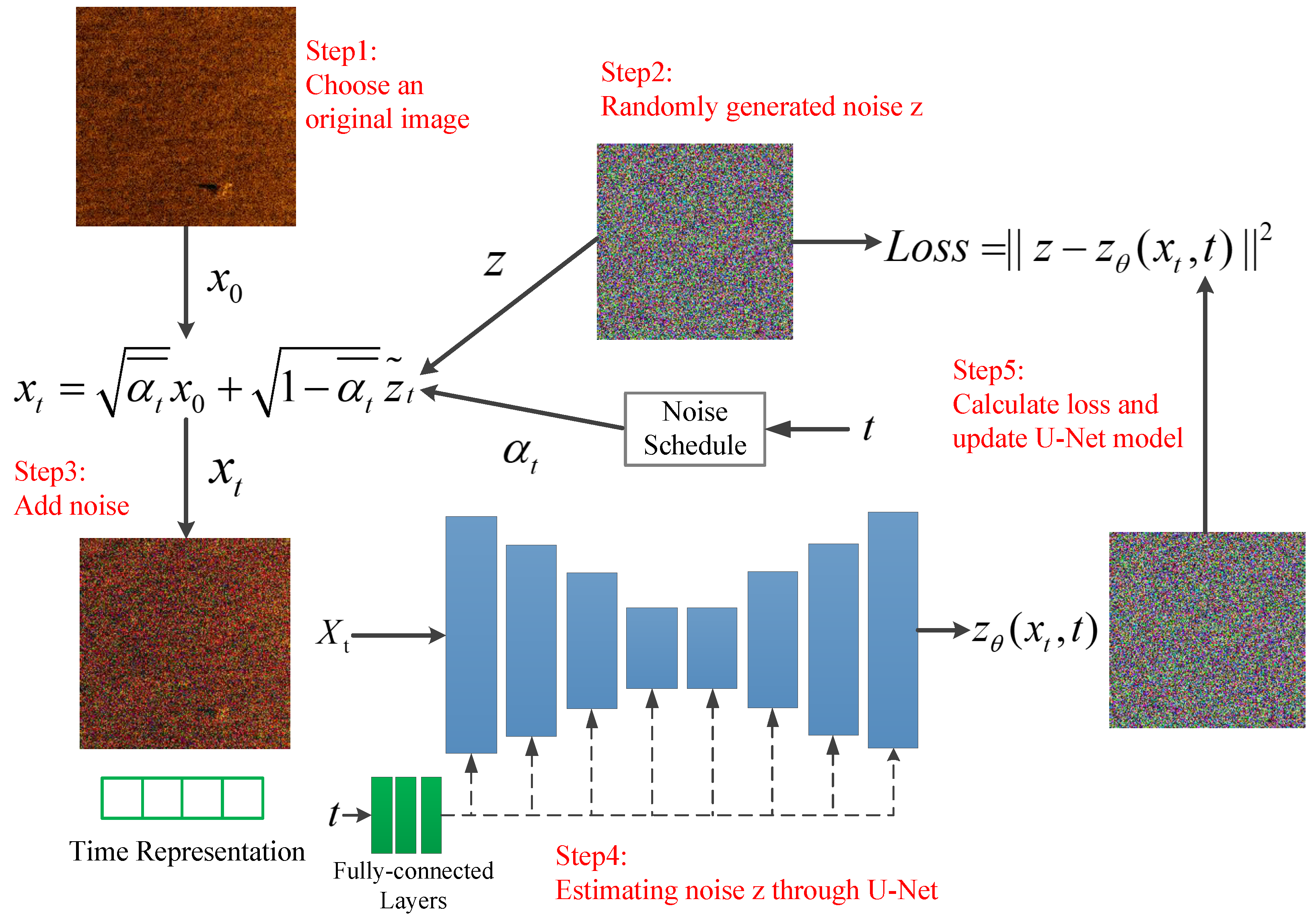
2.1. Denoising Diffusion Probabilistic Models

The diffusion model is currently one of the major focal points in the study of generative models. Its essence lies in continuously adding noise to data, transforming it into realistic noise, and then progressively denoising it to restore the original image. During this process, the model learns the characteristics of the noise and approximates the distribution of the original data. Finally, it can perform random sampling based on the obtained distribution of the original data, generating diverse types of data. The diffusion model used in this paper is DDPM, and the DDPM consists of a forward process and a reverse process, as illustrated in Figure 1. The essence of the forward process is to continuously add standard Gaussian noise, z, to the sonar images until the sonar images become pure-noise images. The essence of the reverse process is to gradually restore the noisy image to the original image by estimating the noise, z.

2.1.1. Forward Process

The forward process involves continuously adding Gaussian noise to the input sonar data. At each time step, Gaussian noise, z, is added, and the image at the next time step is obtained by adding noise to the image from the previous time step. This can be represented by the following formula:
x t = α t x t 1 + 1 α t z 1 x t 1 = α t 1 x t 2 + 1 α t 1 z 2
where α t = 1 β t is the weight term, which ensures that the image diffuses with approximately the same magnitude at each step.
However, if we calculate it recursively step by step, it becomes computationally cumbersome and is not conducive to network training. Therefore, we need a simplified computational approach. By rearranging Equation (1), we can express it as the following formula:
x t = α t ( α t 1 x t 2 + 1 α t 1 z 2 ) + 1 α t z 1
Here, z 1 and z 1 are both standard Gaussian distributions, so we can simplify Equation (2) as follows:
x t = α t α t 1 x t 2 + 1 α t α t 1 z ˜ 1 = α t α t 1 α t 2 x t 3 + 1 α t α t 1 α t 2 z ˜ 2 = α t ¯ x 0 + 1 α t ¯ z ˜ t
where α t ˜ represents the cumulative product, z ˜ 1 , and z ˜ 2 , and z ˜ t are all Gaussian distributions.
With Formulation (3), the distribution at any time step can be computed based on the initial value, x 0 , avoiding the computational complexity associated with recursive calculations.

2.1.2. Reverse Process

The process of reverse engineering involves inferring the distribution of x 0 when x t is known. We cannot directly compute x 0 based on x t ; instead, we first calculate x t 1 using Bayes formula, which can be expressed as follows:
q ( x t 1 | x t ) = q ( x t | x t 1 ) q ( x t 1 ) q ( x t )
For convenience in calculations, let us introduce x 0 , denoted as:
q ( x t 1 | x t , x 0 ) = q ( x t | x t 1 , x 0 ) q ( x t 1 | x 0 ) q ( x t | x 0 )
From the forward process, we can obtain:
q ( x t 1 | x 0 ) = α ¯ t 1 x 0 + 1 α ¯ t 1 z
q ( x t | x 0 ) = α ¯ t x 0 + 1 α ¯ t z
q ( x t | x t 1 , x 0 ) = α t x t 1 + 1 α t z
Since z follows a standard Gaussian distribution, we can infer that:
q ( x t 1 | x 0 ) N ( α ¯ t 1 x 0 , 1 α ¯ t 1 )
q ( x t | x 0 ) N ( α ¯ t x 0 , 1 α ¯ t )
q ( x t | x t 1 , x 0 ) N ( α t x t 1 , 1 α t )
Substituting Equations (6)–(8) into Equation (4), we have:
q ( x t 1 | x t ) exp ( 1 2 ( ( x t α t x t 1 ) 2 β t + ( x t 1 α ¯ t 1 x 0 ) 2 1 α ¯ t 1 ( x t α ¯ t x 0 ) 2 1 α ¯ t ) ) exp ( 1 2 ( ( α t β t + 1 1 α ¯ t 1 ) x t 1 2 ( 2 α t β t x t + 2 α ¯ t 1 1 α ¯ t 1 x 0 ) x t 1 + C ( x t , x 0 ) ) )
Assuming q ( x t 1 | x t ) N ( μ , σ 2 ) , we can obtain from Equation (12):
1 σ 2 = α t β t + 1 1 α ¯ t 1 2 μ σ 2 = 2 α t β t x t + 2 α ¯ t 1 1 α ¯ t 1 x 0
Since α t , β t , and 1 α ¯ t 1 are known, we can directly solve for σ 2 . Furthermore, in the forward process, we can compute x 0 from Equation (3). By substituting x 0 into Equation (13), we can calculate μ :
μ = 1 α t ( x t β t 1 α ¯ t z t )
The distribution parameter, z t , in q ( x t 1 | x t ) is the only remaining parameter yet to be determined. To approximate z t , we can utilize a U-Net-based neural network. In the forward process, the randomly generated z t serves as the ground truth label, and it is compared with the predicted z ˜ t to construct a loss function. By training the network, we can solve for z t . This process is depicted in Figure 2. The noise, z, cannot be directly calculated using a mathematical formula. Therefore, the noise, z, from the forward process is used as the label to train a neural network based on U-Net architecture, aiming to approximate the real noise.
Once we have determined the values of μ and σ 2 , we can also determine the distribution of x t 1 . With this information, we can sample from the distribution of x t 1 to generate images similar to x t 1 . Continuing to propagate forward, we can obtain the image of x 0 .

2.2. Improved YOLOv7 Model

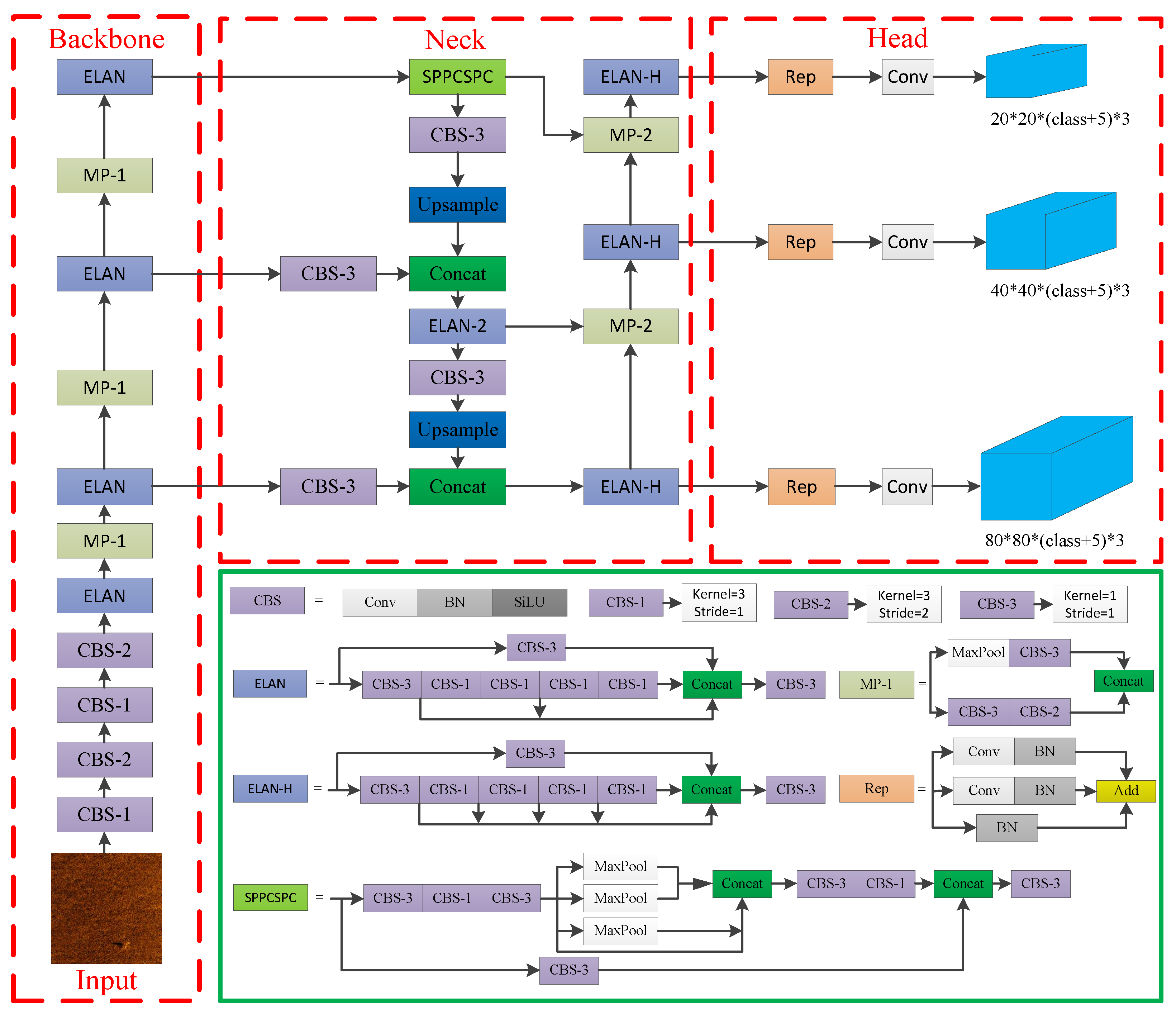
2.2.1. YOLOv7 Overview

The YOLOv7 model is a one-stage detection network proposed in 2022 [35]. Compared to previous models, it achieves higher detection accuracy, faster speed, and better adaptability. As a result, many researchers have made improvements based on YOLOv7 and applied it to their respective domains, yielding good results [36,37].
The network structure of YOLOv7 can be divided into four parts: input, backbone network, neck network, and head network, as shown in Figure 3. The input part preprocesses the images, including data augmentation and resizing to a unified size. The backbone network of yolov7 consists of three modules: MP1, CBS, and ELAN. The role of the backbone network is to extract high-level features from the original images using convolution and pooling operations. The neck network of YOLOv7 combines FPN and PAN structures, which include modules such as SPPCSPC, ELAN-H, MP2, and CBS. The neck network is the layer between the backbone network and the head network. Its purpose is to enhance feature extraction, fuse features from different layers of the backbone network, and adjust the channel number of feature maps to facilitate better integration with the head network. The head network of YOLOv7 controls the channel number using the Rep structure and employs detection heads representing large, medium, and small target sizes to handle objects of different scales. The role of the head network is to map the features extracted by the neck network to the final output, predicting the categories and locations of the targets.

2.2.2. Efficient Channel Attention

In the SSS image, the proportion of effective targets is small, so the feature extraction network generates a large number of negative samples. This abundance of negative samples results in a significant increase in its loss function, which dominates the overall loss function. This situation is unfavorable for model convergence and may lead to the learning of incorrect features. To address these challenges, this study proposes integrating attention mechanisms into the YOLOv7 model to enhance its feature extraction capability and improve localization and object recognition accuracy.
Attention mechanisms are inspired by the human visual attention system, which allows for the efficient processing of image information by selectively focusing on relevant regions of interest, even with limited resources. Prominent attention mechanisms, such as ECA-Net [38], CA [39], BAM [40], SE-Net [41], and CBAM [42], have been shown to enhance the performance of detection models [43,44].
The structure of the ECA-Net attention module is illustrated in Figure 4. Notably, ECA-Net overturns the traditional approach of increasing complexity to improve detection performance. It achieves significant performance improvements by introducing only a small number of additional parameters. Furthermore, ECA-Net is a local cross-channel interaction strategy that does not require dimensionality reduction. Its basic idea is to adaptively adjust the weights of channels by learning their correlations, thereby avoiding the negative impact of dimensionality reduction and effectively achieving cross-channel interaction. ECA-Net employs a one-dimensional convolution with a kernel size of K, where K represents the coverage range of local cross-channel interactions. To avoid the inconvenience of manually adjusting the value of K, a method is designed to automatically calculate K based on the channel dimension. The calculation formula is as follows:
K = φ ( C ) = l o g 2 ( C ) γ + b γ o d d
Here, C represents the channel dimension, o d d denotes the nearest odd number, and γ and b are empirical values generally set to 2 and 1, respectively.
To enhance the detection accuracy of the YOLOv7 model while minimizing the number of model parameters, this paper improves the model’s performance by incorporating the ECA-Net attention module into a specific region of the YOLOv7 model’s neck. The modified YOLOv7 network is illustrated in Figure 5. By adding five ECA modules to the neck network of the initial YOLOv7 network, we enhance the feature extraction capability without modifying the structure of the backbone network. As a result, we can still utilize pre-trained weights for the network.

3. Results

To validate the proposed method for SSS image generation and the improved YOLOv7 model, we first compared it with image generation methods based on DDPM and several GAN-based methods. By comparing the quality of generated images and conducting quantitative analysis, we confirmed the stability and effectiveness of the DDPM-based method in generating small-sample underwater data. Subsequently, we augmented the training set with data generated using DDPM and tested it on popular detection networks as well as our improved YOLOv7 detection network. This further demonstrated that training the network with data generated using DDPM can improve the detection accuracy of the network while also highlighting the superiority of our improved YOLOv7 detection network in SSS object detection.
The proposed method was implemented on a system with the following specifications: Intel(R) Xeon(R) Platinum 8255C CPU with 2.50 GHz, 24 GB of RAM, Nvidia GeForce RTX 3090, CUDA 11.3, Ubuntu 20.04 operating system, 64 bits, and the PyTorch framework.

3.1. Model Evaluation Metrics

The most commonly used evaluation metrics for generative models are Inception Score (IS), Fréchet Inception Distance (FID), and Perceptual Path Length (PPL). However, the Inception Net-V3 model used in calculating the IS metric is trained on the ImageNet dataset, which does not include underwater images. Therefore, the IS metric is not suitable for assessing the quality of the generated images in this study. The PPL metric utilizes the VGG network and focuses on whether the generator can effectively separate and recombine the features of different images. This metric is typically used in face detection and is not applicable to the SSS images generated in this study. On the other hand, the FID metric, although also utilizing the Inception Net-V3 model, directly considers the distance between generated and real data at the feature level. It does not rely on an additional classifier, making it suitable for evaluating the SSS images generated in this study. Therefore, only the FID metric is used as the measure of the generated image quality in this study.
The formula for calculating the FID metric is as follows:
F I D = | | μ r μ g | | 2 + T r ( r + g 2 ( r g ) 1 12 2 )
where μ r represents the mean of the features of real images, μ g represents the mean of the features of generated images, r represents the covariance matrix of real images, g represents the covariance matrix of generated images, and T r represents the trace of the matrices.
A smaller FID value indicates a closer resemblance between the generated distribution and the real image distribution.
To evaluate the performance improvement in the detection model by incorporating generated data and the detection effectiveness of the improved YOLOv7 model, we utilize precision (P), recall (R), and mean Average Precision ( m A P ) as evaluation metrics. The calculation formulas are defined as follows:
R = T P / ( T P + F N )
P = T P / ( T P + F P )
A P = 0 1 P ( R ) d R
m A P = i = 1 N A P i / N
where true positive ( T P ) is the number of correctly detected positive samples, false positive ( F P ) is the number of falsely detected negative samples, and false negative ( F N ) is the number of undetected positive samples. N is the number of detected categories.

3.2. Dataset Preparation

During the data collection phase, we utilized a 324-caliber AUV equipped with an SSS to navigate through designated areas where pre-placed targets were deployed, following a predetermined route. The AUV and the SSS utilized in the experiment are depicted in Figure 6.
To achieve real-time processing of SSS images, we employ a strategy of extracting image segments from the sonar waterfall plot every 30 s, as shown in Figure 7. Additionally, the targets occupy a very small proportion of the entire SSS image. Directly inputting the entire image into the network for training would generate a large number of negative samples, which would impact the training process and waste computational resources. To address this issue, we crop the images into small patches of size 200 × 200 and each patch overlaps by 50 pixels to prevent loss of target features. From these patches, we select the ones that contain targets for training, thus avoiding irrelevant backgrounds that may introduce negative samples. Similarly, during the detection phase, we perform the same cropping operation before feeding the entire image into the detection network.
Due to the uncertainty of sea conditions, collecting data at sea is extremely challenging. After analysis and comparison, we successfully collected 388 valid target images, including 53 cone targets, 55 cylinder targets, and 280 non-preset seabed targets that could cause interference. This dataset exhibits a significant class imbalance issue, and the data volume is limited. We set the ratio of the training set, validation set, and test set to 0.6:0.2:0.2 to maximize the number of samples, and we refer to this original dataset as DatasetA.
Next, we used the DDPM method to generate data. By selecting similar data from the generated dataset, we increased the total number of cone and cylinder data to match the non-targets, which is 280. To ensure a fair comparison of the experimental results, the generated data were only used for the training set, while the quantity of the validation set and test set remained unchanged. The dataset with the added generated data is referred to as DatasetB. The sample counts of DatasetA and DatasetB are shown in Table 1.
Finally, based on the two aforementioned datasets, the effectiveness of the generated data was tested on different detection networks.

3.3. Comparison of Data Generated by DDPM and GANs

Our experimental goal is to generate target-containing images that are similar to the original data in order to increase the sample size of the training set and improve the performance of the detection model. In the experiment, we compared the adversarial autoencoder (AAE), auxiliary classifier GAN (ACGAN), boundary-seeking GAN (BGAN), and DDPM methods. The images generated by the DDPM algorithm and GANs are shown in Figure 8.
From the generated results, it can be observed that the DDPM algorithm produces SSS data with a high degree of similarity to the original data, even when trained with limited data. However, the image quality generated by the GAN method is relatively poor. The GAN approach only generates some background information without producing the desired target images, and it may even suffer from mode collapse.
To quantitatively analyze the similarity between the data generated by the DDPM method and the real data, we calculated the FID metric for the generated and real images, as shown in Table 2. In terms of classification similarity index (dim = 768), the difference between the generated data and the original data extracted by the neural network is very small. These results indicate that the generated synthetic sonar images have a high similarity to the real images. Furthermore, we computed eight Haralick textural features [45] (angular second moment, contrast, correlation, inverse difference moment, sum entropy, entropy, difference variance, and difference entropy) for both datasets and used the multidimensional scaling (MDS) method to measure the texture dissimilarity in two dimensions, as depicted in Figure 9. The vertical and horizontal axes are dimensionless and represent the degree of texture differences. The results show that the generated data exhibit similar texture features to the real sonar data in three different categories and overall.

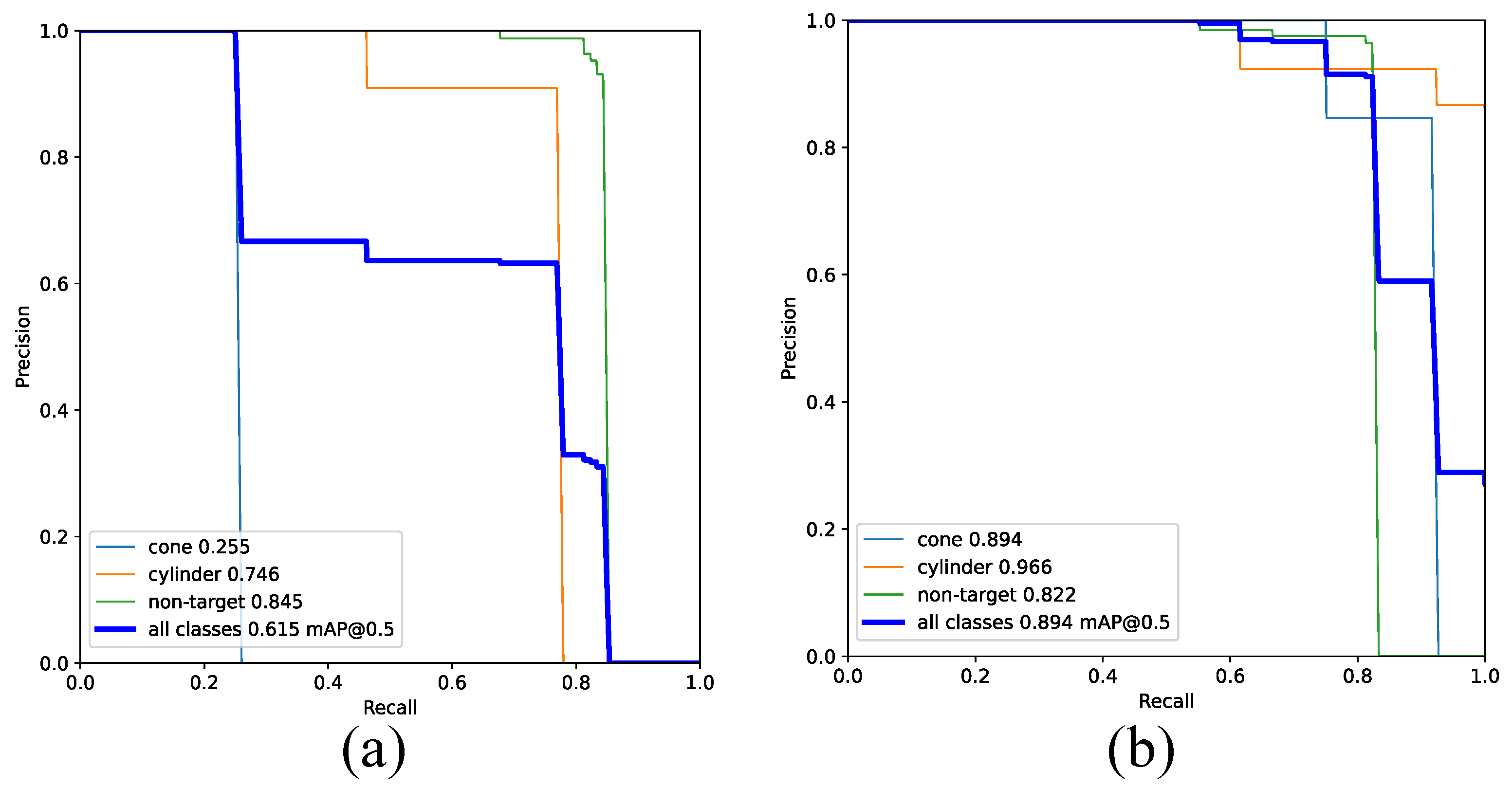
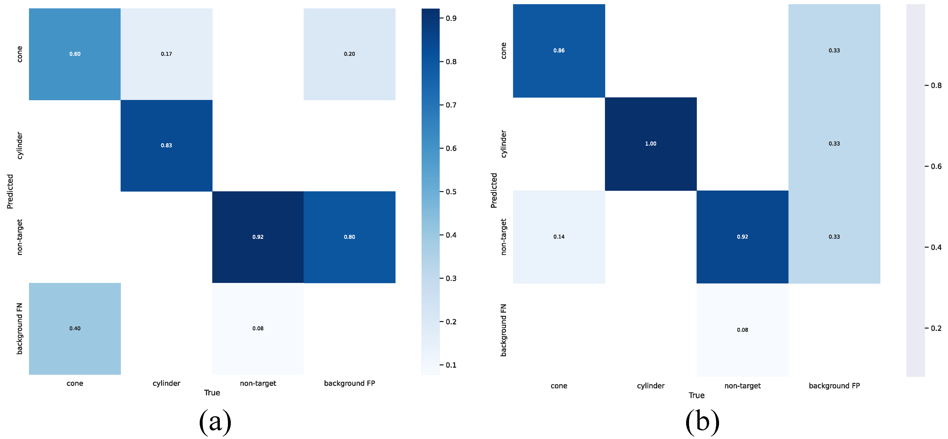
3.4. Performance Comparison of YOLOv7 Networks Trained with DatasetA and DatasetB

In the experiment, our objective is to generate data that are highly similar to real SSS images. However, the most important aspect is to improve the detection performance of our detection network. Therefore, we trained two YOLOv7 models using DatasetA and DatasetB separately (detailed information about the two datasets can be found in Table 1) and compared the detection performance of the two models.
We conducted a comprehensive comparison of the two trained models using the test set. The comparative results from the confusion matrices are presented in Figure 10. The outcomes from the confusion matrix demonstrate the remarkable performance of the network trained on DatasetB, showcasing enhanced accuracy and balance in detecting target and background classes.
In order to further analyze model performance, we examined the PR curves, as presented in Figure 11. Notably, the network trained on DatasetB demonstrated a significantly higher mAP for detection when compared to the network trained on DatasetA. The [email protected] value exhibited an impressive increase of 27.9%.
A visualization of detection results is illustrated in Figure 12. Clearly, the network trained on DatasetB exhibited outstanding performance, surpassing its counterpart trained on DatasetA by successfully detecting more targets and achieving higher accuracy on the test set.
For a comprehensive view of the specific metrics, refer to Table 3. It provides a detailed breakdown of the performance measures, further reinforcing the superiority of the network trained on DatasetB over DatasetA.

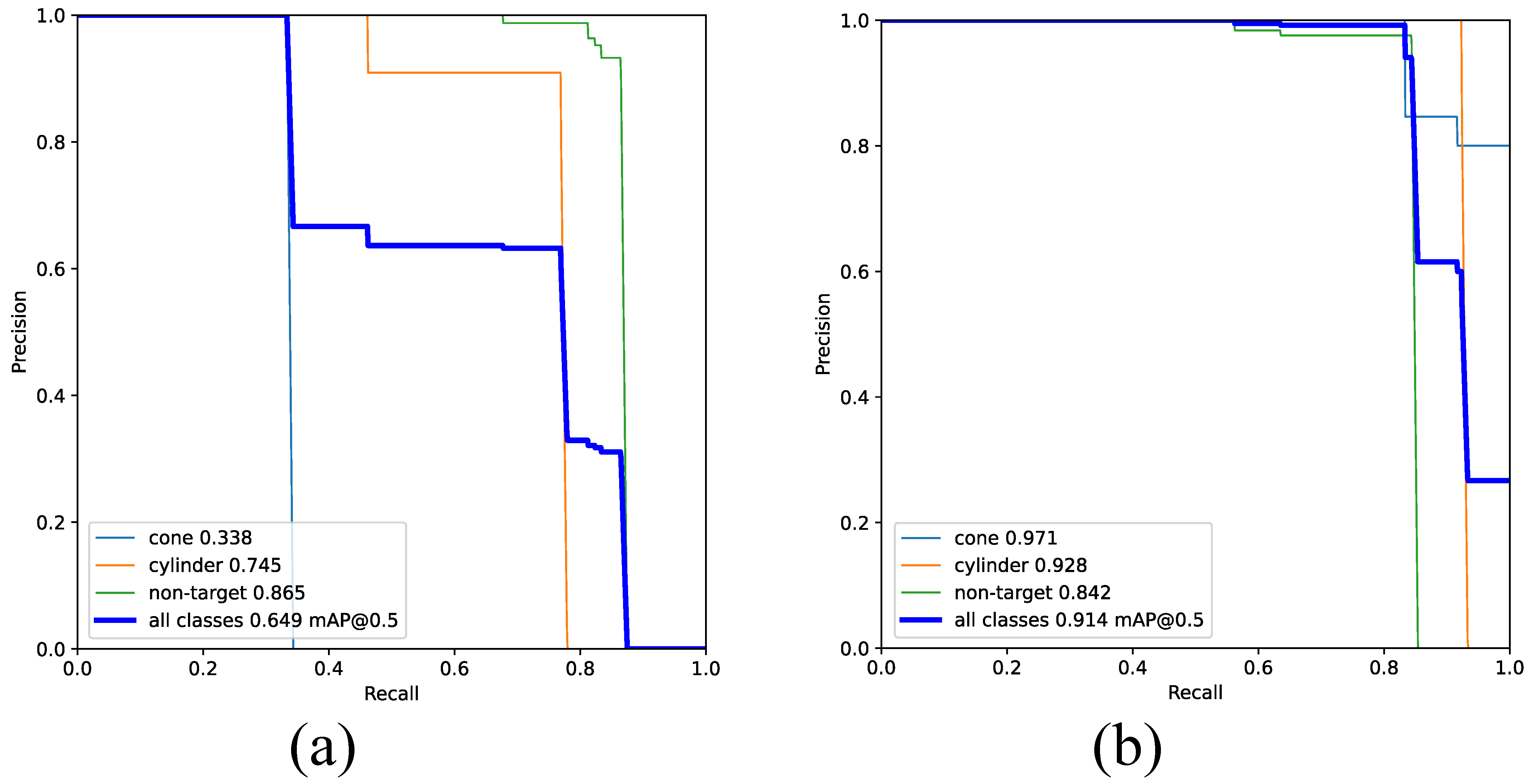
3.5. Performance Comparison of YOLOv7 Integrated with Different Attention Mechanisms

In order to investigate the performance of various commonly used attention mechanisms when integrated with YOLOv7, we individually incorporated each attention mechanism at the same position within the YOLOv7 network. Performance tests were conducted on both the original dataset and the augmented dataset, and the results are presented in Table 4.
From Table 4, it can be observed that incorporating attention mechanisms does not necessarily improve the detection performance of the network. Inappropriate attention mechanisms, on the contrary, can lead to a decrease in the network’s detection performance. Simultaneously, we can also discern that, for the dataset and YOLOv7 network used in this study, ECA and CA exhibit better performance, both of which significantly enhance the network’s detection capabilities. However, when comparing these two attention mechanisms, ECA introduces fewer additional parameters. Therefore, in situations where there is a similar improvement in performance, adding ECA is a preferable choice for underwater platforms with limited computational resources.

3.6. Performance Comparison of Improved YOLOv7 Network against Original YOLOv7 and Other Networks

To validate the performance of our proposed improved YOLOv7 model, we conducted training and testing on DatasetA and DatasetB, respectively. A comparison of the confusion matrices of the improved models on the test set is shown in Figure 13, and the PR curves are illustrated in Figure 14. Compared with Figure 10 and Figure 11, our improved model has higher detection accuracy on both datasets. The detection results of the improved models are depicted in Figure 15. A comparison of the detection results with those shown in Figure 12 illustrates that the improved YOLOv7 network achieves accurate detection for objects that were either missed or incorrectly identified by the original YOLOv7 network, as demonstrated in images 10.png and 15.png. These findings affirm the improved YOLOv7 network’s superior detection performance and efficacy.
The specific metrics are provided in Table 5. Compared to Table 3, the improved model achieved varying degrees of improvement in the mAP metric on the test set. On DatasetA, the [email protected] increased by 3.4%, while on DatasetB, the [email protected] improved by 2%.
Additionally, we conducted a comparative analysis of the improved YOLOv7 network with several commonly used underwater object detection networks, including Faster-RCNN, SSD, EfficientDet-D0, DETR, YOLOv5, and YOLOv7. Specific comparison metrics are detailed in Table 6. The data provided in the table strongly validate the effectiveness of the proposed data augmentation method. Employing our approach to enhance training data significantly improved the detection performance of the model. Furthermore, the results confirm the superior performance of our improved YOLOv7 model in detecting acoustic small targets.
We also compared our improved YOLOv7 network with Co-DETR, a state-of-the-art network trained on the COCO dataset. From the data in Table 6, it can be observed that our improved YOLOv7 network and Co-DETR network perform similarly on our dataset, with Co-DETR showing better performance in the mAP.5:.95 metric on DatasetB. It can be anticipated that with more fine-tuning of Co-DETR, its detection performance on our dataset is likely to surpass that of our improved YOLOv7. However, it should be noted that Co-DETR has a parameter count of 348 million, nearly ten times that of our improved YOLOv7 network (37 million). This makes the application of Co-DETR on underwater platforms with limited computational resources highly challenging. Therefore, to ensure the deployment and use of models on underwater platforms, we often make a trade-off by sacrificing some detection performance and opting for more lightweight networks.

4. Discussion

From Figure 8 and Figure 9 and Table 2, it can be observed that DDPM performs well in generating underwater small-sample SSS data. Compared to GAN networks, the diffusion model is easier to train and can generate images similar to the original dataset even with limited raw data. From Table 3, Table 5 and Table 6, it can be seen that training the detection model with generated images significantly improves the mAP metric. However, since the diffusion model generates data based on the learned probability distribution, the probability of generating targets with few samples in the original data is also low. In this study, a total of 18,000 images were generated, and 480 images were selected for data augmentation. This selection process involves a certain level of subjectivity, but it is completely acceptable compared to the training difficulties and mode collapse issues of GAN networks.
Furthermore, from Table 3, Table 5 and Table 6, it can also be observed that the improved YOLOv7 model in this paper has better detection performance, with significant improvements in detection metrics and actual detection results. However, there are still some errors in object detection, such as in Figure 15, where the model detects the cone in 12.png as a cylinder and misses a non-target in 14.png. This is because different objects in sonar images can have very similar characteristics, posing a major challenge in underwater acoustic target detection.
In summary, the diffusion model has great potential in underwater applications. It is well known that underwater data collection is costly and challenging. The advantage of the diffusion model lies in its ability to generate data based on small samples and its stable training process. This can significantly reduce the cost of data acquisition, making it highly suitable for underwater target detection tasks.

5. Conclusions

This paper leveraged SSS images collected by AUV to generate data using DDPM and compared it with the GAN method. The results demonstrated the superiority of the diffusion model in generating small-sample underwater datasets. Additionally, an SSS small-target dataset was constructed, addressing the challenges and high costs associated with underwater target data collection. Furthermore, considering the characteristics of small underwater target data, improvements were made to the YOLOv7 network by incorporating an ECANet attention module to enhance feature extraction capabilities. Finally, the generated data were added to the training set, and tests were conducted on mainstream detection networks as well as our improved YOLOv7 network. The results validated that training the network and adding the generated data improves detection accuracy, with an mAP increase of approximately 30% across different detection networks. Moreover, the superiority of the improved YOLOv7 network in detecting small underwater targets was confirmed, with a 2.0% mAP improvement compared to the original network.
Additionally, this study had certain limitations. Firstly, in the generation of side-scan sonar images using the diffusion model, the process of generating a substantial amount of data and then selecting high-quality data for augmenting training samples is highly time-consuming and not suitable for real-time online generation. On the other hand, the improved YOLOv7 network introduced in this paper may sometimes make errors in recognizing different samples with very high similarity. However, we believe that in cases where there has not been a significant improvement in side-scan sonar imaging accuracy, identifying such highly similar but distinct samples is a challenging task, which is a common issue in underwater acoustic target detection. Finally, in terms of the dataset used, this study employed a relatively small number of samples. This limitation could potentially prevent some networks from fully demonstrating their performance. However, in the field of underwater acoustic target detection, data collection is inherently challenging. Therefore, conducting detection tasks with limited data aligns well with real-world engineering demands.
In future work, we plan to incorporate lightweight network techniques to reduce model complexity and improve the speed of generating images and detecting targets. The aim is to adapt to underwater platforms with limited computational resources. Additionally, we will conduct more experiments, collect more data, expand the dataset, and enhance the diversity of target categories within the dataset to accommodate a broader range of underwater target detection scenarios.

Author Contributions

Conceptualization, C.C. and F.Z.; methodology, C.C. and X.H.; coding, C.C., X.H., and X.W.; experiment design, C.C., F.Z., and W.L.; writing—original draft preparation, C.C.; writing—review and editing, F.Z. and W.L. All authors have read and agreed to the published version of the manuscript.

Funding

This study was supported by the National Natural Science Foundation of China (52171322), the National Key Research and Development Program (2020YFB1313200), the Fundamental Research Funds for the Central Universities (D5000210944), and the Graduate Innovation Fund (PF2023066).

Data Availability Statement

The data presented in this study are available upon request from the corresponding author.

Acknowledgments

We would like to acknowledge the facilities and technical assistance provided by the Key Laboratory of Unmanned Underwater Transport Technology.

Conflicts of Interest

The authors declare no conflict of interest.

References

  1. Li, J.; Chen, L.; Shen, J.; Xiao, X.; Liu, X.; Sun, X.; Wang, X.; Li, D. Improved Neural Network with Spatial Pyramid Pooling and Online Datasets Preprocessing for Underwater Target Detection Based on Side Scan Sonar Imagery. Remote Sens. 2023, 15, 440. [Google Scholar] [CrossRef]
  2. Wu, M.; Wang, Q.; Rigall, E.; Li, K.; Zhu, W.; He, B.; Yan, T. ECNet: Efficient convolutional networks for side scan sonar image segmentation. Sensors 2019, 19, 2009. [Google Scholar] [CrossRef] [PubMed]
  3. Yu, Y.; Zhao, J.; Gong, Q.; Huang, C.; Zheng, G.; Ma, J. Real-time underwater maritime object detection in side-scan sonar images based on transformer-YOLOv5. Remote Sens. 2021, 13, 3555. [Google Scholar] [CrossRef]
  4. Szymak, P.; Piskur, P.; Naus, K. The effectiveness of using a pretrained deep learning neural networks for object classification in underwater video. Remote Sens. 2020, 12, 3020. [Google Scholar] [CrossRef]
  5. Li, L.; Li, Y.; Yue, C.; Xu, G.; Wang, H.; Feng, X. Real-time underwater target detection for AUV using side scan sonar images based on deep learning. Appl. Ocean Res. 2023, 138, 103630. [Google Scholar] [CrossRef]
  6. Long, H.; Shen, L.; Wang, Z.; Chen, J. Underwater Forward-Looking Sonar Images Target Detection via Speckle Reduction and Scene Prior. IEEE Trans. Geosci. Remote. Sens. 2023, 61, l5604413. [Google Scholar] [CrossRef]
  7. Doersch, C. Tutorial on variational autoencoders. arXiv 2016, arXiv:1606.05908. [Google Scholar]
  8. Kingma, D.P.; Welling, M. An introduction to variational autoencoders. Foundations and Trends® in Machine Learning; Now Publishers: Hanover, MD, USA, 2019; Volume 12, pp. 307–392. [Google Scholar]
  9. Alias, A.G.; Ke, N.R.; Ganguli, S.; Bengio, Y. Variational walkback: Learning a transition operator as a stochastic recurrent net. In Advances in Neural Information Processing Systems, Proceedings of the 31st Annual Conference on Neural Information Processing Systems (NIPS 2017), Long Beach, CA, USA, 4–9 December 2017; Curran Associates Inc.: Red Hook, NY, USA, 2017; Volume 30, p. 30. [Google Scholar]
  10. Kim, T.; Bengio, Y. Deep directed generative models with energy-based probability estimation. arXiv 2016, arXiv:1606.03439. [Google Scholar]
  11. Goodfellow, I.; Pouget-Abadie, J.; Mirza, M.; Xu, B.; Warde-Farley, D.; Ozair, S.; Courville, A.; Bengio, Y. Generative adversarial networks. Commun. ACM 2020, 63, 139–144. [Google Scholar] [CrossRef]
  12. Creswell, A.; White, T.; Dumoulin, V.; Arulkumaran, K.; Sengupta, B.; Bharath, A.A. Generative adversarial networks: An overview. IEEE Signal Process. Mag. 2018, 35, 53–65. [Google Scholar] [CrossRef]
  13. Gui, J.; Sun, Z.; Wen, Y.; Tao, D.; Ye, J. A review on generative adversarial networks: Algorithms, theory, and applications. IEEE Trans. Knowl. Data Eng. 2021, 35, 3313–3332. [Google Scholar] [CrossRef]
  14. Kobyzev, I.; Prince, S.J.; Brubaker, M.A. Normalizing flows: An introduction and review of current methods. IEEE Trans. Pattern Anal. Mach. Intell. 2020, 43, 3964–3979. [Google Scholar] [CrossRef]
  15. Papamakarios, G.; Nalisnick, E.; Rezende, D.J.; Mohamed, S.; Lakshminarayanan, B. Normalizing flows for probabilistic modeling and inference. J. Mach. Learn. Res. 2021, 22, 2617–2680. [Google Scholar]
  16. Saharia, C.; Chan, W.; Chang, H.; Lee, C.; Ho, J.; Salimans, T.; Fleet, D.; Norouzi, M. Palette: Image-to-image diffusion models. In Proceedings of the ACM SIGGRAPH 2022 Conference, Los Angeles, CA, USA, 6–10 August 2022; pp. 1–10. [Google Scholar]
  17. Ho, J.; Jain, A.; Abbeel, P. Denoising diffusion probabilistic models. Advances in Neural Information Processing Systems: 34th Annual Conference on Neural Information Processing Systems (NeurIPS 2020), Virtual Conference, 6–12 December 2020; Volume 33, pp. 6840–6851. [Google Scholar]
  18. Chen, Y.; Liang, H.; Pang, S. Study on small samples active sonar target recognition based on deep learning. J. Mar. Sci. Eng. 2022, 10, 1144. [Google Scholar] [CrossRef]
  19. Xu, Y.; Wang, X.; Wang, K.; Shi, J.; Sun, W. Underwater sonar image classification using generative adversarial network and convolutional neural network. IET Image Process. 2020, 14, 2819–2825. [Google Scholar] [CrossRef]
  20. Wang, Z.; Guo, Q.; Lei, M.; Guo, S.; Ye, X. High-Quality Sonar Image Generation Algorithm Based on Generative Adversarial Networks. In Proceedings of the 2021 40th Chinese Control Conference (CCC), IEEE, Shanghai, China, 26–28 July 2021; pp. 3099–3104. [Google Scholar]
  21. Jegorova, M.; Karjalainen, A.I.; Vazquez, J.; Hospedales, T. Full-scale continuous synthetic sonar data generation with markov conditional generative adversarial networks. In Proceedings of the 2020 IEEE International Conference on Robotics and Automation (ICRA), Paris, France, 31 May–31 August 2020; pp. 3168–3174. [Google Scholar]
  22. Jiang, Y.; Ku, B.; Kim, W.; Ko, H. Side-scan sonar image synthesis based on generative adversarial network for images in multiple frequencies. IEEE Geosci. Remote. Sens. Lett. 2020, 18, 1505–1509. [Google Scholar] [CrossRef]
  23. Lee, E.h.; Park, B.; Jeon, M.H.; Jang, H.; Kim, A.; Lee, S. Data augmentation using image translation for underwater sonar image segmentation. PLoS ONE 2022, 17, e0272602. [Google Scholar] [CrossRef] [PubMed]
  24. Liu, D.; Wang, Y.; Ji, Y.; Tsuchiya, H.; Yamashita, A.; Asama, H. Cyclegan-based realistic image dataset generation for forward-looking sonar. Adv. Robot. 2021, 35, 242–254. [Google Scholar] [CrossRef]
  25. Zhang, Z.; Tang, J.; Zhong, H.; Wu, H.; Zhang, P.; Ning, M. Spectral Normalized CycleGAN with Application in Semisupervised Semantic Segmentation of Sonar Images. Comput. Intell. Neurosci. 2022, 2022, 1274260. [Google Scholar] [CrossRef]
  26. Karjalainen, A.I.; Mitchell, R.; Vazquez, J. Training and validation of automatic target recognition systems using generative adversarial networks. In Proceedings of the 2019 Sensor Signal Processing for Defence Conference (SSPD), Brighton, UK, 9–10 May 2019; pp. 1–5. [Google Scholar]
  27. Ho, J.; Salimans, T.; Gritsenko, A.; Chan, W.; Norouzi, M.; Fleet, D.J. Video diffusion models. arXiv 2022, arXiv:2204.03458. [Google Scholar]
  28. Batzolis, G.; Stanczuk, J.; Schönlieb, C.B.; Etmann, C. Conditional image generation with score-based diffusion models. arXiv 2021, arXiv:2111.13606. [Google Scholar]
  29. Chen, T.; Zhang, R.; Hinton, G. Analog bits: Generating discrete data using diffusion models with self-conditioning. arXiv 2022, arXiv:2208.04202. [Google Scholar]
  30. Alcaraz, J.M.L.; Strodthoff, N. Diffusion-based time series imputation and forecasting with structured state space models. arXiv 2022, arXiv:2208.09399. [Google Scholar]
  31. Liu, J.; Li, C.; Ren, Y.; Chen, F.; Zhao, Z. Diffsinger: Singing voice synthesis via shallow diffusion mechanism. In Proceedings of the AAAI Conference on Artificial Intelligence, Virtual Conference, 22 February–1 March 2022; Volume 36, pp. 11020–11028. [Google Scholar]
  32. Koizumi, Y.; Zen, H.; Yatabe, K.; Chen, N.; Bacchiani, M. SpecGrad: Diffusion probabilistic model based neural vocoder with adaptive noise spectral shaping. arXiv 2022, arXiv:2203.16749. [Google Scholar]
  33. Cao, H.; Tan, C.; Gao, Z.; Chen, G.; Heng, P.A.; Li, S.Z. A survey on generative diffusion model. arXiv 2022, arXiv:2209.02646. [Google Scholar]
  34. Luo, S.; Su, Y.; Peng, X.; Wang, S.; Peng, J.; Ma, J. Antigen-specific antibody design and optimization with diffusion-based generative models. bioRxiv 2022. [Google Scholar] [CrossRef]
  35. Wang, C.Y.; Bochkovskiy, A.; Liao, H.Y.M. YOLOv7: Trainable bag-of-freebies sets new state-of-the-art for real-time object detectors. arXiv 2022, arXiv:2207.02696. [Google Scholar]
  36. Liu, K.; Sun, Q.; Sun, D.; Peng, L.; Yang, M.; Wang, N. Underwater target detection based on improved YOLOv7. J. Mar. Sci. Eng. 2023, 11, 677. [Google Scholar] [CrossRef]
  37. Chen, X.; Yuan, M.; Yang, Q.; Yao, H.; Wang, H. Underwater-YCC: Underwater Target Detection Optimization Algorithm Based on YOLOv7. J. Mar. Sci. Eng. 2023, 11, 995. [Google Scholar] [CrossRef]
  38. Wang, Q.; Wu, B.; Zhu, P.; Li, P.; Zuo, W.; Hu, Q. ECA-Net: Efficient channel attention for deep convolutional neural networks. In Proceedings of the IEEE/CVF Conference on Computer Vision and Pattern Recognition, Seattle, WA, USA, 13–19 June 2020; pp. 11534–11542. [Google Scholar]
  39. Hou, Q.; Zhou, D.; Feng, J. Coordinate attention for efficient mobile network design. In Proceedings of the IEEE/CVF Conference on Computer Vision and Pattern Recognition, Nashville, TN, USA, 20–25 June 2021; pp. 13713–13722. [Google Scholar]
  40. Park, J.; Woo, S.; Lee, J.Y.; Kweon, I.S. Bam: Bottleneck attention module. arXiv 2018, arXiv:1807.06514. [Google Scholar]
  41. Hu, J.; Shen, L.; Sun, G. Squeeze-and-excitation networks. In Proceedings of the IEEE Conference on Computer Vision and Pattern Recognition, Salt Lake City, UT, USA, 18–23 June 2018; pp. 7132–7141. [Google Scholar]
  42. Woo, S.; Park, J.; Lee, J.Y.; Kweon, I.S. Cbam: Convolutional block attention module. In Proceedings of the European Conference on Computer Vision (ECCV), Munich, Germany, 8–14 September 2018; pp. 3–19. [Google Scholar]
  43. Zhang, M.; Yin, L. Solar cell surface defect detection based on improved YOLO v5. IEEE Access 2022, 10, 80804–80815. [Google Scholar] [CrossRef]
  44. Sitaula, C.; KC, S.; Aryal, J. Enhanced Multi-level Features for Very High Resolution Remote Sensing Scene Classification. arXiv 2023, arXiv:2305.00679. [Google Scholar]
  45. Zhang, Z.; Yan, Z.; Jing, J.; Gu, H.; Li, H. Generating Paired Seismic Training Data with Cycle-Consistent Adversarial Networks. Remote Sens. 2023, 15, 265. [Google Scholar] [CrossRef]
Figure 1. Schematic diagram of DDPM method.
Remotesensing 15 04772 g001
Figure 2. The addition and calculation process of noise, z.
Remotesensing 15 04772 g002
Figure 3. The network structure of initial YOLOv7.
Remotesensing 15 04772 g003
Figure 4. ECA-Net network structure.
Remotesensing 15 04772 g004
Figure 5. The network structure of improved YOLOv7.
Remotesensing 15 04772 g005
Figure 6. The AUV and the SSS utilized in the experiment.
Remotesensing 15 04772 g006
Figure 7. Preprocessing of SSS images.
Remotesensing 15 04772 g007
Figure 8. Image generated by DDPM and GANs method. (a) Original SSS images. (b) DDPM method. (c) AAE method. (d) ACGAN method. (e) BGAN method.
Remotesensing 15 04772 g008
Figure 9. Relative texture dissimilarity of generated data and real data. (a) The generated cone and the real cone. (b) The generated cylinder and the real cylinder. (c) The generated non-target and the real non-target. (d) All generated data and all real data.
Remotesensing 15 04772 g009
Figure 10. Comparison of confusion matrices for YOLOv7 networks trained on DatasetA and DatasetB on the test set. (a) Network trained using DatasetA. (b) Network trained using DatasetB.
Remotesensing 15 04772 g010
Figure 11. Comparison of PR curves for YOLOv7 networks trained on DatasetA and DatasetB on the test set. (a) Network trained using DatasetA. (b) Network trained using DatasetB.
Remotesensing 15 04772 g011
Figure 12. Comparison of detection results for YOLOv7 networks trained on DatasetA and DatasetB on the test set. (a) Ground truth labels. (b) Network trained using DatasetA. (c) Network trained using DatasetB.
Remotesensing 15 04772 g012
Figure 13. Comparison of confusion matrices for improved YOLOv7 networks trained on DatasetA and DatasetB on the test set. (a) Network trained using DatasetA. (b) Network trained using DatasetB.
Remotesensing 15 04772 g013
Figure 14. Comparison of PR curves for improved YOLOv7 networks trained on DatasetA and DatasetB on the test set. (a) Network trained using DatasetA. (b) Network trained using DatasetB.
Remotesensing 15 04772 g014
Figure 15. Comparison of detection results for improved YOLOv7 networks trained on DatasetA and DatasetB on the test set. (a) Ground truth labels. (b) Network trained using DatasetA. (c) Network trained using DatasetB.
Remotesensing 15 04772 g015
Table 1. The number of samples in the initial dataset and the augmented dataset.
CategoryDatasetADatasetB
TrainValTestTotalTrainValTestTotal
Cone301112532571112280
Cylinder301213552551213280
Non-target16856562801685656280
Table 2. The FID metric for generated data by DDPM and real data.
MethodConeCylinderNon-TargetAll Data
FID (dim = 64)2.170.690.110.39
FID (dim = 192)4.641.370.250.87
FID (dim = 768)0.200.160.130.08
FID (dim = 2048)59.5156.8436.9431.51
Table 3. Performance comparison of the YOLOv7 model trained on DatasetA and DatasetB on the test set.
CategoryDatasetADatasetB
PrecisionRecallmAP.5mAP.5:.95PrecisionRecallmAP.5mAP.5:.95
All0.9300.6210.6150.2900.8770.9020.8940.517
Cone1.0000.2500.2550.1530.8440.9170.8940.577
Cylinder0.9090.7690.7460.3880.8121.0000.9660.583
Non-target0.9310.8440.8450.3290.9740.7880.8220.392
Table 4. Performance comparison of YOLOv7 integrated with different attention mechanisms.
MethodDatasetADatasetB
PrecisionRecallmAP.5mAP.5:.95PrecisionRecallmAP.5mAP.5:.95
YOLOv70.9300.6210.6150.2900.8770.9020.8940.517
YOLOv7+SE0.9230.6470.6320.2970.8990.9180.9100.521
cYOLOv7+BAM0.9350.6200.6140.2850.8780.8970.8960.515
cYOLOv7+CBAM0.9370.6320.6450.3080.8840.9010.8930.519
cYOLOv7+CA0.9250.6540.6530.3110.9020.9240.9170.523
cYOLOv7+ECA0.9280.6530.6490.3120.9030.9220.9140.524
Table 5. Performance comparison of the improved YOLOv7 model trained on DatasetA and DatasetB.
CategoryDatasetADatasetB
PrecisionRecallmAP.5mAP.5:.95PrecisionRecallmAP.5mAP.5:.95
All0.9280.6530.6490.3120.9030.9220.9140.524
Cone1.0000.3330.3380.2120.8001.0000.9710.628
Cylinder0.8520.7690.7450.3880.9230.9230.9280.557
Non-target0.9320.8580.8650.3370.9760.8440.8420.388
Table 6. Performance comparison of different detection models trained on DatasetA and DatasetB.
MethodDatasetADatasetB
PrecisionRecallmAP.5mAP.5:.95PrecisionRecallmAP.5mAP.5:.95
SSD0.8610.7060.5870.2790.8790.9040.8860.468
DETR0.9130.6350.6120.2880.9100.9170.8760.499
Faster-RCNN0.8820.6890.6020.2430.8240.8360.8570.471
EfficientDet-D00.9310.6430.6100.2990.8850.9160.8990.518
YOLOv50.9050.6170.6230.2960.8790.8990.9010.513
YOLOv70.9300.6210.6150.2900.8770.9020.8940.517
Co-DETR0.9250.5100.6420.3110.8990.9240.9100.526
YOLOv7+ECA0.9280.6530.6490.3120.9030.9220.9140.524
Disclaimer/Publisher’s Note: The statements, opinions and data contained in all publications are solely those of the individual author(s) and contributor(s) and not of MDPI and/or the editor(s). MDPI and/or the editor(s) disclaim responsibility for any injury to people or property resulting from any ideas, methods, instructions or products referred to in the content.

