Communication

A Sound Velocity Prediction Model for Seafloor Sediments Based on Deep Neural Networks

1
School of Ocean Engineering and Technology, Sun Yat-sen University, Zhuhai 519000, China
2
Key Laboratory of Comprehensive Observation of Polar Environment (Sun Yat-sen University), Ministry of Education, Zhuhai 519082, China
3
Key Laboratory of Marine Geology and Metallogeny, First Institute of Oceanography, MNR, No. 6 Xianxialing Road, Laoshan District, Qingdao 266061, China
*
Author to whom correspondence should be addressed.
Remote Sens. 2023, 15(18), 4483; https://doi.org/10.3390/rs15184483
Submission received: 31 July 2023 / Revised: 22 August 2023 / Accepted: 5 September 2023 / Published: 12 September 2023
(This article belongs to the Section Ocean Remote Sensing)

Abstract

:
The acoustic properties of seafloor sediments have always been important parameters in sound field analyses and exploration for marine resources, and the accurate acquisition of the acoustic properties of sediments is one of the difficulties in the study of underwater acoustics. In this study, sediment cores were taken from the northern South China Sea, and the acoustic properties were analyzed. Since traditional methods (such as regression equations or theoretical models) are difficult to apply in practical engineering applications, we applied remote sensing data to sound velocity prediction models for the first time. Based on the influencing mechanism of the acoustic properties of seafloor sediments, the sediments’ source, type and physical properties have a great influence on the acoustic properties. Therefore, we replaced these influencing factors with easily accessible data and remote sensing data, such as parameters of granularity, distance to the nearest coast, decadal average sea surface productivity, water depth, etc., using deep neural networks (DNN) to develop a sound velocity prediction model. Compared with traditional mathematical analyses, the DNN model improved the accuracy of prediction and can be applied to practical engineering applications.

1. Introduction

The acoustic properties of seafloor sediments are more complex than those of seawater and rocks, since they have the acoustic properties of both particle skeletons and pore fluids [1,2,3,4], and they are closely related to the characteristics of the deposition environment, the structural characteristics of the sediment, and the physical and mechanical properties [5,6,7,8].
In the past few decades, based on many laboratory sampling measurements and data measured in situ, some outstanding results in the field of acoustic wave theory have been achieved. Hamilton published a series of studies on sediment’s acoustic properties and summarized the viscoelastic model based on the correlation between the acoustic properties and the physical parameters [9]. Hamilton’s empirical model showed that the velocity of sound is approximately independent of the frequency, and that the attenuation of sound increases linearly with the frequency (from a few hertz to a few megahertz) but at high frequencies (>10 kHz) or for fine-grained sediments with high porosity, the values of acoustic attenuation calculated by Hamilton’s model do not agree with the experimental values [1,9]. Considering that the interaction between the pore fluid and the elastic frame would lead to the viscous resistance of acoustic waves, Biot first proposed the Biot theory that is applicable to porous elastic media, and Stoll et al. established and improved the Biot–Stoll model [10,11,12]. The Biot–Stoll model predicts that the attenuation of sound in sediments should exhibit nonlinear frequency dependence, especially at the bottom of sandy and sand–mud mixtures, and that the velocity of sound in these sediments should exhibit a strong nonlinear dispersion [12]. Buckingham [13,14] proposed the GS (grain-shearing) and VGS (viscous grain-shearing) models based on the interaction between sediment particles and the viscosity of thin layers of intergranular pore fluid molecules. He argued that the unconsolidated particles of the two phases were regarded as a continuum that contained no elastic framework and only intergranular stresses. BICSQS (Biot–Stoll with Squirt Flow and Biot–Stoll with Squirt Flow) was proposed by Chotiros and Isakson and uses a physical model of particle-to-particle contact (including jet flow and shear resistance) to calculate the frame’s modulus to explain the dispersion of acoustic velocity in existing published experimental data of saturated sandy sediments [5]. Based on Biot theory, Williams proposed the EDFM (effective density fluid) model [15]. In the EDFM model, the porous medium is approximated as a fluid with a fluid modulus and effective density, the frame’s volume modulus and shear modulus are set to zero, and only the propagation of compression waves in the sediment is considered [15].
Although the theoretical models above can be used for predicting sediment’s acoustic parameters, there are too many input parameters, such as 13 input parameters in the Biot model. Furthermore, some parameters in the theoretical models are difficult to measure, such as the bending of the porosity factor, or cannot be accurately measured, such as the frame’s modulus. Therefore, when theoretical models are applied to practical problems, they are often limited by the difficulty of obtaining the input parameters. Another commonly used method for predicting the velocity of sound is the regression equation, but like the theoretical models, the input parameters of the regression equations are also difficult to obtain, so it is difficult to carry out practical applications. Hou et al. first proposed using machine learning methods in models predicting the velocity of sound, and he used the traditional physical parameters to test the random forest algorithm, which has given us a new way to study geo-acoustic properties [16]. In the subsequent research, they proposed that combining multiple parameters of particle size to build a prediction model on the basis of physical parameters could further improve the predictions’ accuracy [17]. Chen et al. also used the XGBoost algorithm to study the prediction model [18]. However, the input parameters in these prediction models are still hard to obtain or contain data that are hard to obtain.
To solve the problem that the input parameters are difficult to obtain, we wondered whether remote sensing data could be applied to predicting the velocity of sound and establish a multiple parameter model to solve the problems in practical application. Therefore, combined with the machine learning method, based on analyzing the influencing mechanism of the acoustic properties and comprehensively considering various parameters that affect the acoustic properties, we proposed a method of acquiring the velocity of sound for seafloor sediments based on remote sensing information in this study.

2. Data Acquisition and Conditioning

2.1. Acoustic Data and Input Parameters

The seafloor’s surface sediment cores were obtained with a gravity corer and/or a box corer on cruises and were taken by the South China Sea Institute of Oceanology, Chinese Academy of Sciences. The velocity of sound was measured with a portable WSD-4 digital sonic instrument and the coaxial differential distance measurement method under standard conditions (23 °C, atmospheric pressure) [6,19]. The laboratory measurements were calibrated to the seafloor values by using the ratio of the velocity of sound [1,6]. The sediment’s particle density was measured by the pycnometer method, and the wet density was measured by the ring knife method, The main equipment used was (1) a ring knife with an inner diameter of 61.8 mm and a height of 20 mm, and a (2) balance able to weigh 500 g an a minimum indexing value of 0.1 g. The moisture content test was calculated from the loss of weight, and the porosity was calculated using the particle’s specific gravity and water content. The parameters of granularity, such as the sand, silt, and clay content; the mean grain size (Mz) and the median particle size (Md), were measured with a particle size analyzer by the South China Sea Institute of Oceanology Chinese Academy of Sciences.
The resulting dataset contained 77 locations of the seafloor’s surface sediments in the northern SCS. The main sediment types are clayey silt, silty clay, and sand–silt–clay. The locations are mainly distributed in the northern SCS’s continental shelf and slope, and the deepest water depth is deeper than 1500 m.
The acoustic properties of the seafloor’s sediment are affected by many factors, such as the types and sources of the sediment. However, these influencing factors cannot be directly inputted into a model or regression equations, so we needed to convert these influencing factors into data that can be directly processed. Details of the process are shown in the results section.

2.2. Machine Learning Method: Deep Neural Networks

Machine learning (ML) language is a scientific study of algorithms and statistical models. It originates from the study of pattern recognition and computational learning theory in artificial intelligence. It imitates the mechanism of the human brain to interpret data and learn data. In the past few years, ML technology has been successfully applied in many different fields, such as self-driving systems, remote sensing and computer vision. Deep neural networks (DNN) are one of the most widely used ML algorithms, and they have become a powerful tool for ML and artificial intelligence.
DNN are artificial neural networks (ANN) with multiple hidden layers between the input and output layers. These networks are based on a set of layers connected to each other. DNNs can model complex nonlinear relationships and are widely used in supervised learning and reinforcement learning problems. Here, we used DNN to study the relationship between the influencing factors and the velocity of sound.
In a DNN, each layer (input or output) has basic nodes, and each node is a perception mimicking a neuron (Figure 1). Usually, we used multilayered perception (MLP) with at least three layers. Each layer is modified by a set of weights and biases, each layer has a unique weight, and each node has a unique bias. The predictive accuracy of each layer depends on its weights and biases. With the output of hidden layers denoted by h(l)(x), the computation for a network with L hidden layers is [20]:
f(x) = f[a(L+1) (h(L)(a(L) (… (h(2) (a(2) (h(1) (a(1)(x))))))))]
Each pre-activation function a(l)(x) is typically a linear operation with the matrix W(l) and a bias of b(l).
In supervised learning, the input data should be trained in each layer before being output, and the training process will improve the accuracy of the neural network. The output values of a regression network will be compared with the real value, and the difference is called the cost function or the loss function. A cost function is a single value that is the sum of the deviation of the model from the real value for all points in the dataset.
J W , b , x , y = 1 2 | | a L y | | 2 2
where aL and y are the vectors of the characteristic dimension n_out, and ||S||2 is the L2 norm of S. The training process aims to make the loss function as small as possible; that is, in each layer, the network tweaks the weights and biases until the prediction matches the correct output. The trained model can be saved and to make an accurate prediction at another time. The weight matrix W and the bias b satisfy the following formula:
a L = σ ( W L a L 1 + b L )
For the parameters of the output layer, the cost function becomes
J W , b , x , y = 1 2 | | σ ( W L a L 1 + b L ) y | | 2 2
The weights matrix W and the bias b of layer L can be calculated by the gradient descent method:
(1)
Initialize the linear relationship between each hidden layer and output layer. The values of W and b are random values.
(2)
For iteration to 1 to max:
(2-1)
for I = 1 to m:
(a)
Set a1 to xi;
(b)
For l = 2 to L, use forward propagation calculation
a i , l = σ ( W l a i , l 1 + b l )
(c)
Calculate the δi,l of output layer by the cost function;
(d)
For l = L to 2, backpropagation calculation is performed
δ i , l = ( W l + 1 ) T δ i , l + 1 σ ( z i , l )
(2-2)
For l = 2 to L, update Wl and bl at layer L
W L = W L a i = 1 m δ i , l a i , l 1 T
b L = b L a i = 1 m δ i , l
(2-3)
If all the change values of W and B are less than the threshold of stopping iteration, the iteration cycle will be skipped.
Training DNNs consist of the following basic steps [21,22]:
Step 1: Weight initialization: Initialize the weights and biases. A neural network has many parameters, so the parameters must be initialized before training the network. Good initialization can avoid the occurrence of gradient dispersion and gradient explosion, accelerating the network’s training.
Step 2: Forward propagation: The given input parameter matrix should be normalized before forward propagation; then, for every layer, compute a linear combination of normalized inputs and weights and then apply the activation function to the linear combination a(l)(x). The final layer gives the prediction y_pre.
Step 3: Compute the loss function: Neural networks rely on loss values to generate gradients to update the weights. The loss function is the error between the actual values and the predicted values, and our main objective is to minimize the loss function.
Step 4: Backpropagation: In backpropagation, we use the loss value obtained in the previous step to calculate the gradient and propagate the gradient to the previous layer to update the weights.
Step 5: Repeat Steps 2–4 for n epochs until we observe that the loss function is minimized without overfitting the training data.

2.3. Feature Input

Through an analysis of the influencing mechanism of the acoustic properties of the seafloor’s sediments, we found that the acoustic properties of the seafloor’s sediments are affected by a variety of macro- and microfactors, including the source of the sediment, the topography and geomorphology, the type of sediment, the hydrodynamic conditions, etc., while the microfactors are mainly the physical properties of the sediment [6]. To enable the DNN model to be used in practice, we input data that are easy to obtain to represent these factors into the model for training.
According to the sand–silt–clay ratio [23], the sediment type can be determined by the granular components of the sediment, that is, the sand, silt and clay contents. The sources of the bottom sediments are mainly divided into terrigenous and biogenic sources. Terrigenous materials are generally transported by hydrodynamic conditions, and the transport of sediment is related to the grain size, the water’s depth and the offshore distance. The process of transporting sediment is carried out in accordance with the process of differentiating the sediment’s granularity, namely, from the shore to the sea. With an increase in the source of sediment and the transportation distance, the ocean’s dynamic conditions gradually weaken, and the trend of the sediment’s particle size becomes smaller. Larger sediments are deposited in the nearshore estuary and inland shelf, while better sorted sediments are carried along with the flow, with only a small number of fine particles carried to the outer shelf and beyond. The characteristics of the grain size of the sediments are among the basic properties of sediments and are the result of the comprehensive effects of the topography, geomorphology, hydrodynamic conditions and transportation distance of the sediments. The grain size of the sediments contains abundant information such as the transport path of the sediments, the climate and the environment. Therefore, the information on the topography, geomorphic hydrodynamic conditions and provenance of the sediments can be analyzed through multiple parameters of the sediment’s grain size. In addition, biogenic sediments are also one of the sediment sources, and biogenic sediments are mainly affected by the primary productivity of the sea surface. The physical properties are closely related to the sediment’s acoustic properties, and porosity is the main factor affecting the acoustic properties of sediments [1].

3. Results

On the basis of the analysis above, we replaced these influencing factors with easily accessible data and remote sensing data, such as the sediment type, parameters of granularity, distance to the nearest coast, decadal average sea surface productivity, and water depth. The detailed input parameters and data sources are shown in Table 1. The velocity of sound; wet bulk density; porosity; sand, silt and clay content; mean grain size (Mz) and median particle size (Md) were measured in the laboratory. The distance to the nearest coast was calculated from the Global Self-consistent, Hierarchical, High-resolution Geography Database from NOAA’s National Centers for Environmental Information [24]. The water’s depth was obtained from the Global Bathymetry and Topography at 15 arc sec [25]. The average primary productivity was recalculated from the Remote Sensing of Oceanic Primary Productivity [26].
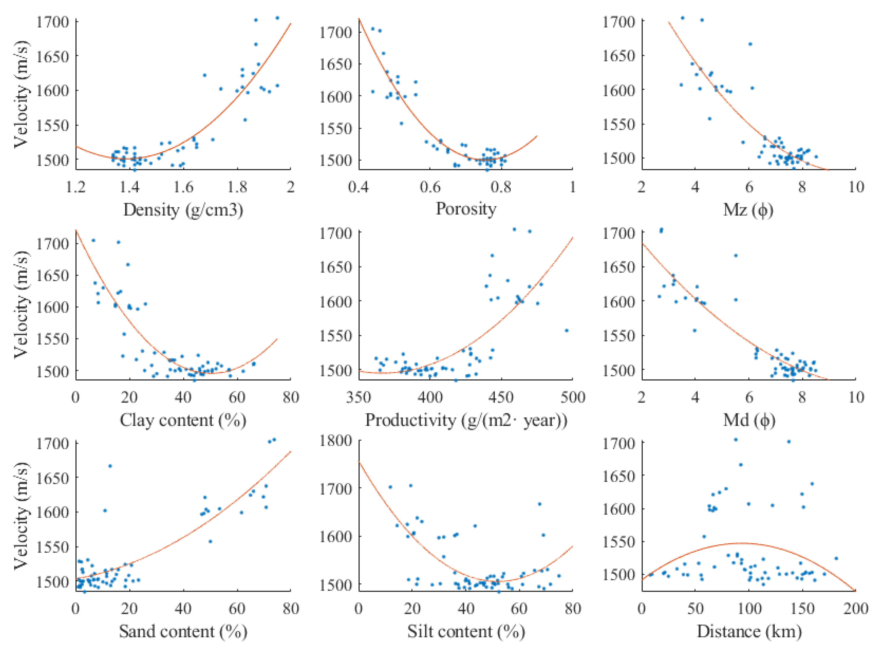
The regression equations between the velocity of sound and the input parameters was established by using the least squares method, and the training data and the correlation between the velocity of sound and the input parameters are shown in Figure 2. According to Figure 2, some input parameters have a good quadratic relationship with the velocity of sound. The exponential and linear functions can be seen in the Supplementary Materials, and all the R2 values were reduced even when we used an exponential function and a linear function independently; thus we chose the quadratic relationship for the comparison with the machine learning method in this study. For example, porosity is negatively correlated with the velocity of sound, and the velocity of sound decreased with increasing porosity, which is consistent with porosity–velocity relationships [1,19]. We used the traditional quadratic regression method for fitting the regression of the input parameters, and the single-parameter regression equations are listed in Table 2. The highest coefficient of determination (R2) of the single-parameter regression equation was 0.89, and the lowest was as low as 0.05. If two or more parameters were analyzed simultaneously, the accuracy was even lower. This is the advantage of ML algorithms, which can handle multidimensional parameters at the same time. ML algorithms can analyze the internal relationships between each parameter, and the more parameters there are, the more accurate the analysis.
In this article, we used DNN to establish a predictive model for the velocity of sound. The total dataset had 77 stations and was divided into the training data and the test dataset. The training data included 65 points, and the test data had 12 points. To avoid overfitting, the dataset was randomly assigned, and we used a test set as an estimate. The input features were wet bulk density; porosity; sand, silt and clay content; mean grain size (Mz); median size (Md); distance to the nearest coast; water depth and annual average primary productivity, for a total of 10 input features (Figure 1 and Table 1). Therefore, the training matrix was a 65 × 10 matrix, the training label (the corresponding measured velocities of sound) was a 65 × 1 vector, the test data were a 12 × 10 matrix and the test label was a 12 × 1 vector.
According to this analysis, the following model training parameters were set:
  • n_hidden_1 = 64; number of neurons in Hidden Layer 1;
  • n_hidden_2 = 64; number of neurons in Hidden Layer 2;
  • n_input = 10; number of input parameters;
  • n_prediction = 1; since the output is the velocity of sound, the number of outputs was 1;
  • training_epochs = 300; number of training cycles;
  • batch_size = 10; the amount of data to be taken per batch.
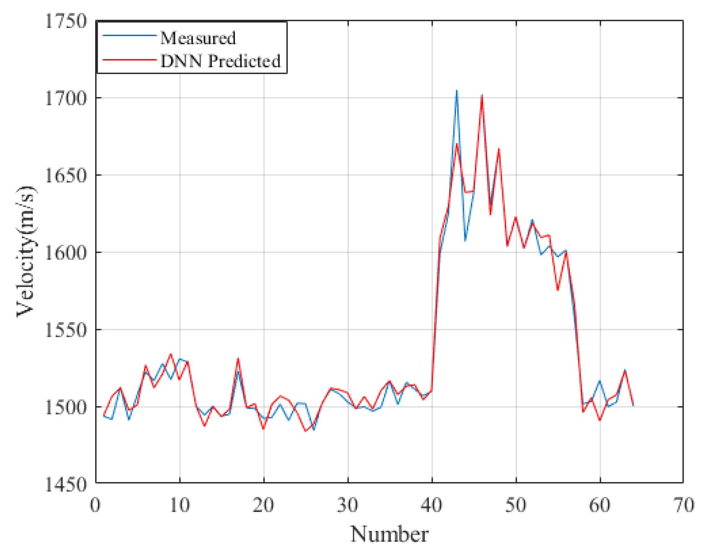
The coefficient of determination (R2) of the DNN model was 0.97, and the training matrix was input into the DNN model. The results are shown in Figure 3. The model’s predicted values are almost consistent with the measured values, which shows that the training results had a good fit to the training dataset.

4. Discussion

From the training dataset, the DNN model could handle 10 parameters simultaneously and had an R2 as high as 0.97, which implies that compared with traditional data analysis methods (regression equations), the DNN has obvious advantages. However, does the trained DNN model have the same accuracy when applied to other areas?
To verify the accuracy of the DNN model, we used 10 test data points from different area for testing, and the results are shown in Figure 4. The comparison between DNN and the conventional regression method for predicting the velocity of sound are shown in Table 3. From Figure 4, we can see that the predicted values of the DNN model had the same trend as the real measured values, and the error was small. In Table 3, we tested the regression equation’s error with the data from the test stations, and the results showed that the velocity of sound–porosity relationship had the highest accuracy among the correlations. The standard deviation (STDEV) of the velocity–porosity regression was 22.66, and the root mean square error (RMSE) was 38.54. Compared with these correlations, the DNN model had more accuracy: the STDEV of the DNN model was 17.67 and the RMSE was 33.73, which shows that the DNN model is more accurate than the regression equations for predicting the velocity of sound.
The input parameters used in the DNN model are mainly easily accessible data, such as the granularity parameters (sand, silt and clay content; Mz and Md) of the seafloor’s sediments in the SCS, which have accumulated after years of collection. Other remote sensing parameters, such as the distance to the nearest coast, the decadal average sea surface productivity and the water’s depth, are also easily accessible data. If we want to predict the velocity of sound in an area, the DNN model can provide a better and more accurate prediction. The importance of the 10 features is provided in the Supplementary Materials.

5. Conclusions

To solve the problem of accuracy in the acquisition of the velocity of sound, we developed a new velocity of sound model based on the DNN method.
(1)
Compared with theoretical models and regression equations, not only can our new model easily take advantage of accessible data, such as remote sensing data, but it can also easily be applied in practice.
(2)
Due to the advantages of machine learning for processing multidimensional data, the DNN model can comprehensively consider various factors affecting the velocity of sound, such as the source of the sediment, the sedimentary environment and the physical properties, compared with traditional methods (regression equations), and thus the DNN model has improved predictive accuracy.
(3)
For the first time, this study shows the possibility of using remote sensing data in geo-acoustics, and it provides a new method for the rapid acquisition of the velocity of sound of sediment.

Supplementary Materials

The following supporting information can be downloaded at https://www.mdpi.com/article/10.3390/rs15184483/s1. Feature importance is used to illustrate the importance of a feature to the model. Figure S1. The feature importance of the 10 features. The feature number and corresponding names are shown in Table 1. Table S1. The regression equations of input parameters in exponential functions. Table S2. The regression equations of input parameters in linear functions. Figures for exponential + linear functions of the input parameters. From the Figures S2 to S11, Figures for exponential + linear functions of the input parameters. Figure S2. Exponential (black line) + linear (red line) functions of density vs sound velocity. Figure S3. Exponential (black line) + linear (red line) functions of porosity vs sound velocity. Figure S4. Exponential (black line) + linear (red line) functions of sand content vs sound velocity. Figure S5. Exponential (black line) + linear (red line) functions of silt content vs sound velocity. Figure S6. Exponential (black line) + linear (red line) functions of clay content vs sound velocity. Figure S7. Exponential (black line) + linear (red line) functions of Mz vs sound velocity. Figure S8. Exponential (black line) + linear (red line) functions of Md vs sound velocity. Figure S9. Exponential (black line) + linear (red line) functions of distance vs sound velocity. Figure S10. Exponential (black line) + linear (red line) functions of depth vs sound velocity. Figure S11. Exponential (black line) + linear (red line) functions of productivity vs sound velocity.

Author Contributions

Methodology, Z.H.; data curation, Z.H., J.W. and G.L.; writing—original draft preparation, Z.H.; writing—review and editing, Z.H. and G.L. All authors have read and agreed to the published version of the manuscript.

Funding

This study was funded by the National Key R&D Program of China (2021YFF0501202), the National Natural Science Foundation of China (12374428, 42176191, 41706045, U22A2012).

Data Availability Statement

The data presented in this study are available on request from the corresponding author.

Conflicts of Interest

The authors declare no conflict of interest.

References

  1. Hamilton, E.L.; Bachman, R.T. Sound velocity and related properties of marine sediments. J. Acoust. Soc. Am. 1982, 72, 1891–1904. [Google Scholar]
  2. Endler, M.; Endler, R.; Wunderlich, J.; Bobertz, B.; Leipe, T.; Moros, M.; Jensen, J.B.; Arz, H. Geo-acoustic modelling of late and postglacial sedimentary units in the Baltic Sea and their acoustic visibility. Mar. Geol. 2016, 376, 86–101. [Google Scholar]
  3. Kan, G.; Zou, D.; Liu, B.; Wang, J.; Meng, X.; Li, G.; Pei, Y. Correction for effects of temperature and pressure on sound speed in shallow seafloor sediments. Mar. Georesources Geotechnol. 2019, 37, 1217–1226. [Google Scholar]
  4. Kim, S.R.; Lee, G.S.; Kim, D.C.; Bae, S.H.; Kim, S.P. Physical properties and geoacoustic provinces of surficial sediments in the southwestern part of the Ulleung Basin in the East Sea. Quat. Int. 2017, 459, 35–44. [Google Scholar]
  5. Chotiros, N.P.; Isakson, M.J. A broadband model of sandy ocean sediments: Biot–Stoll with contact squirt flow and shear drag. J. Acoust. Soc. Am. 2004, 116, 2011–2022. [Google Scholar]
  6. Rajan, S.D.; Lin, Y.T. Broadband Geoacoustic Inversions for Seabed Characterization of the New England Mud Patch. IEEE J. Ocean. Eng. 2022, 48, 264–276. [Google Scholar]
  7. Lee, K.M.; Ballard, M.S.; McNeese, A.R.; Wilson, P.S. Sound speed and attenuation measurements within a seagrass meadow from the water column into the seabed. J. Acoust. Soc. Am. 2017, 141, EL402–EL406. [Google Scholar]
  8. Potty, G.R.; Miller, J.H.; Michalopoulou, Z.H.; Bonnel, J. Estimation of geoacoustic parameters using machine learning techniques. J. Acoust. Soc. Am. 2019, 146, 2987. [Google Scholar]
  9. Hamilton, E.L. Geoacoustic modeling of the sea floor. J. Acoust. Soc. Am. 1980, 68, 1313–1340. [Google Scholar]
  10. Biot, M.A. Theory of Propagation of Elastic Waves in a Fluid-saturated Porous Solid. II. Higher Frequency Range. J. Acoust. Soc. Am. 1956, 28, 179–191. [Google Scholar]
  11. Stoll, R.D. Acoustic waves in ocean sediments. Geophysics 1977, 42, 715–725. [Google Scholar]
  12. Stoll, R.D.; Bautista, E.O. Using the Biot theory to establish a baseline geoacoustic model for seafloor sediments. Cont. Shelf Res. 1998, 18, 1839–1857. [Google Scholar] [CrossRef]
  13. Buckingham, M.J. Wave propagation, stress relaxation, and grain-to-grain shearing in saturated, unconsolidated marine sediments. J. Acoust. Soc. Am. 2000, 108, 2796–2815. [Google Scholar]
  14. Buckingham, M.J. Analysis of shear-wave attenuation in unconsolidated sands and glass beads. J. Acoust. Soc. Am. 2014, 136, 2478–2488. [Google Scholar]
  15. Williams, K.L. Adding thermal and granularity effects to the effective density fluid model. J. Acoust. Soc. Am. 2013, 133, EL431–EL437. [Google Scholar]
  16. Hou, Z.Y.; Wang, J.Q.; Chen, Z.; Yan, W.; Tian, Y.H. Sound velocity predictive model based on physical properties. Earth Space Sci. 2019, 6, 1561–1568. [Google Scholar] [CrossRef]
  17. Wang, J.; Hou, Z.; Li, G.; Kan, G.; Meng, X.; Liu, B. A new compressional wave speed inversion method based on granularity parameters. IEEE Access 2019, 7, 185849–185856. [Google Scholar]
  18. Chen, M.; Meng, X.; Kan, G.; Wang, J.; Li, G.; Liu, B.; Liu, C.; Liu, Y.; Liu, Y.; Lu, J. Predicting the Sound Speed of Seafloor Sediments in the East China Sea Based on an XGBoost Algorithm. J. Mar. Sci. Eng. 2022, 10, 1366. [Google Scholar]
  19. Hou, Z.; Guo, C.; Wang, J.; Chen, W.; Fu, Y.; Li, T. Seafloor sediment study from South China Sea: Acoustic & physical property relationship. Remote Sens. 2015, 7, 570–585. [Google Scholar]
  20. Witten, I.H.; Frank, E. Data mining: Practical machine learning tools and techniques with Java implementations. ACM Sigmod Rec. 2002, 31, 76–77. [Google Scholar] [CrossRef]
  21. Montavon, G.; Samek, W.; Müller, K.R. Methods for interpreting and understanding deep neural networks. Digit. Signal Process. 2018, 73, 1–15. [Google Scholar]
  22. Sze, V.; Chen, Y.H.; Yang, T.J.; Emer, J.S. Efficient processing of deep neural networks: A tutorial and survey. Proc. IEEE 2017, 105, 2295–2329. [Google Scholar] [CrossRef]
  23. Shepard, F.P. Nomenclature based on sand-silt-clay ratios. J. Sediment. Res. 1954, 24, 151–158. [Google Scholar]
  24. Wessel, P.; Smith, W.H.F. A global, self-consistent, hierarchical, high-resolution shoreline. J. Geophys. Res. 1996, 101, 8741–8743. [Google Scholar] [CrossRef]
  25. Smith, W.H.F.; Sandwell, D.T. Global sea floor topography from satellite altimetry and ship depth soundings. Science 1997, 277, 1956–1962. [Google Scholar] [CrossRef]
  26. Tang, S.; Chen, C. Novel maximum carbon fixation rate algorithms for remote sensing of oceanic primary productivity. IEEE J. Sel. Top. Appl. Earth Obs. Remote Sens. 2016, 9, 5202–5208. [Google Scholar] [CrossRef]
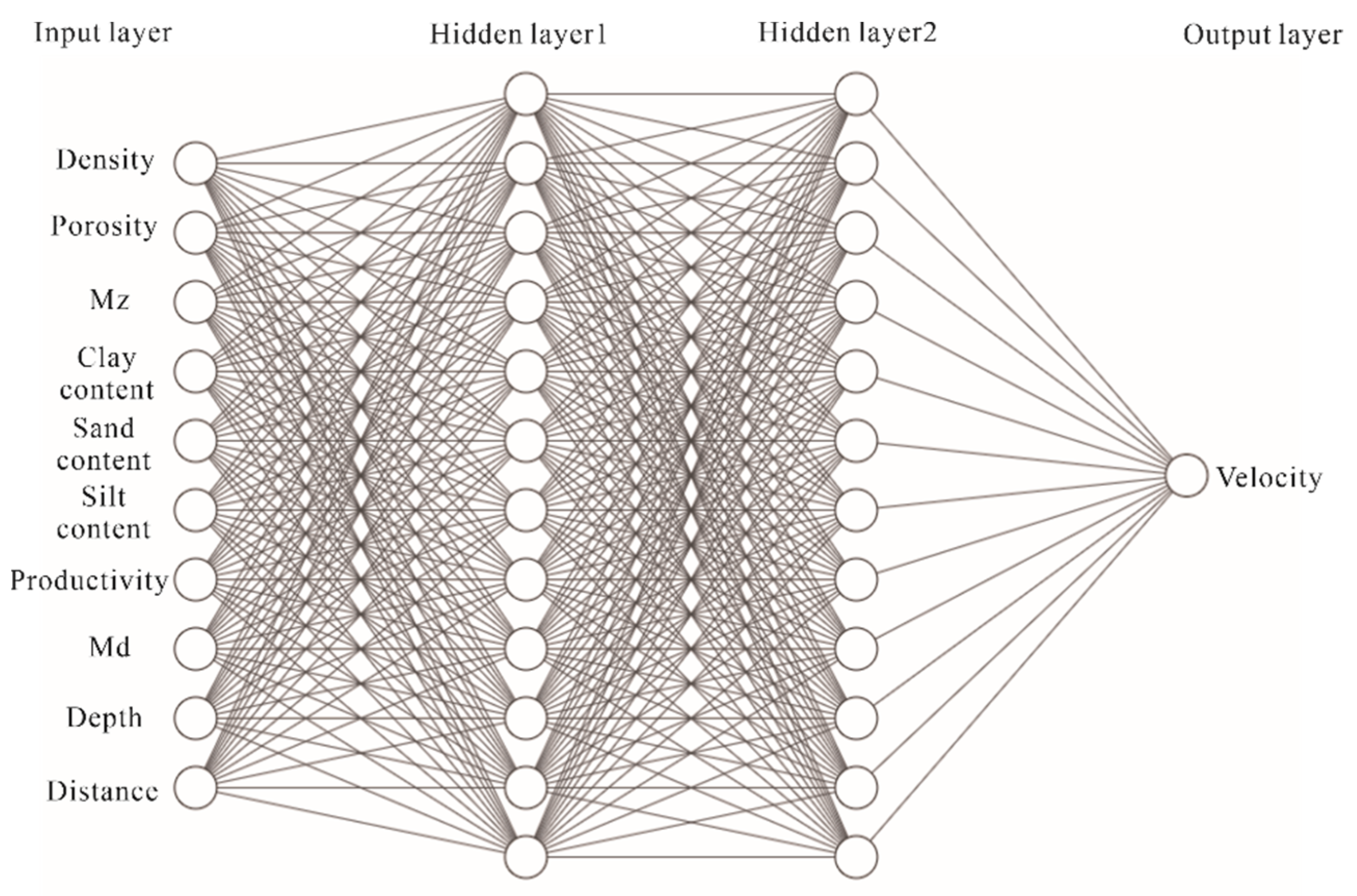
Figure 1. The structure of the input and output layers of DNNs. Here, Hidden Layers 1 and 2 are just an indication that there can be multiple hidden layers.
Remotesensing 15 04483 g001
Figure 2. The correlations between the input parameters (density, porosity, mean grain size (Mz), clay content, productivity, median particle size (Md), sand content, silt content, and distance to the source) and the velocity of sound.
Remotesensing 15 04483 g002
Figure 3. The results of model training compared with the measured values.
Remotesensing 15 04483 g003
Figure 4. The error of the predicted results of regression equations and DNN Model. 1, DNN model; 2, density equation; 3, porosity equation; 4, sand equation; 5, silt equation; 6, clay equation; 7, Mz equation; 8, Md equation; 9, distance equation; 10, depth equation; 11, productivity equation.
Remotesensing 15 04483 g004
Table 1. The input parameters and sources in the study.
ParametersFeature
Numbers
AbbreviationData SourceLabel
Velocity of soundLabelVpLaboratory measurementOutput
Wet bulk densityFeature 0ρLaboratory measurementInput
PorosityFeature 1nLaboratory measurementInput
Sand contentFeature 2sandLaboratory measurementInput
Silt contentFeature 3siltLaboratory measurementInput
Clay contentFeature 4clayLaboratory measurementInput
Mean grain sizeFeature 5MzLaboratory measurementInput
Median sizeFeature 6MdLaboratory measurementInput
Distance to the nearest coastFeature 7disGlobal Self-consistent, Hierarchical, High-resolution
Geography Database from NOAA’s National Centers for Environmental Information [24]
Input
Water depthFeature 8depthSRTM15+ [25]Input
Average primary productivityFeature 9proRemote Sensing of Oceanic Primary Productivity [26]Input
Table 2. The regression equations of the input parameters.
EquationsRegression EquationsR2
Vp = f(ρ)Vp = 524.8ρ2 − 1457ρ + 25120.82
Vp = f(n)Vp = 1765n2 − 2662n + 25040.89
Vp = f(sand)Vp = 0.02036sand2 + 0.685sand + 15030.74
Vp = f(silt)Vp = 0.09307silt2 − 9.651silt + 17560.43
Vp = f(clay)Vp = 0.08951clay2 − 9.006clay + 17220.76
Vp = f(Mz)Vp = 4.57mz2 − 91.02mz + 19310.78
Vp = f(md)Vp = 2.498md2 − 56.15md + 17880.83
Vp = f(dis)Vp = −0.006457dis2 + 1.202dis + 14910.05
Vp = f(depth)Vp = 3.166 × 10⁻⁵ depth2 − 0.1391depth + 16170.65
Vp = f(pro)Vp = 0.01114pro2 − 8.17pro + 29930.58
Table 3. The statistics of the predicted error of the regression equations and the DNN model for the 10 test parameters.
EquationsSTDEVRMSE
Vp = f(ρ)22.5049.90
Vp = f(n)22.6638.54
Vp = f(sand)24.4537.53
Vp = f(silt)24.4537.53
Vp = f(clay)36.6864.75
Vp = f(Mz)22.8051.35
Vp = f(md)27.2453.03
Vp = f(dis)48.0975.15
Vp = f(depth)43.1281.80
Vp = f(pro)388.27439.52
Vp = DNN model17.6733.73
STDEV is the standard deviation; RMSE is the root mean square error.
Disclaimer/Publisher’s Note: The statements, opinions and data contained in all publications are solely those of the individual author(s) and contributor(s) and not of MDPI and/or the editor(s). MDPI and/or the editor(s) disclaim responsibility for any injury to people or property resulting from any ideas, methods, instructions or products referred to in the content.