Article

Statistical Downscaling of SEVIRI Land Surface Temperature to WRF Near-Surface Air Temperature Using a Deep Learning Model

Fraunhofer Institute for Building Physics, Fraunhoferstraße 10, 83626 Valley, Germany
*
Author to whom correspondence should be addressed.
Remote Sens. 2023, 15(18), 4447; https://doi.org/10.3390/rs15184447
Submission received: 4 July 2023 / Revised: 31 August 2023 / Accepted: 7 September 2023 / Published: 9 September 2023
(This article belongs to the Section Urban Remote Sensing)

Abstract

:
The analysis of the near-surface air temperature is vital for many applications such as urban heat islands and climate change studies. In particular, extreme weather events are typically localized and so should the corresponding adaptation measures. However, climate scientists are often confronted with the difficulty of providing reliable predictions at high spatial resolutions in the order of 1 km. We propose to train a convolutional neural network model to emulate the hourly high-resolution near-surface air temperature field simulated by the Weather Research and Forecasting (WRF) software over a period of 18 months. The model is driven by current and past lags of coarse SEVIRI land surface temperature fields. This nowcasting application implements a downscaling of the spatial resolution of the input by about a factor of four, while establishing a correlation between current and past land surface temperature maps and the current near-surface air temperature field. The U-Net variant that is proposed in this study uses regularization to prevent over-fitting and implements a novel space-time approach, where multiple time steps are fed into the model through 3D convolution layers. Besides LST, the model also uses urban density as additional static input to be able to predict the temperature more accurately in urban areas and to improve the generalizability of the trained model. The performance of our U-Net model is assessed via comparison to an MLR benchmark (ridge regularization). The model is shown to be superior on all performance metrics. It achieves a mean absolute error of 1.36 ° C versus 1.49 ° C for benchmark (a 9% relative improvement) and a root mean square error of 1.77 ° C versus 1.91 ° C for benchmark (a 7% relative improvement). The absolute error of the model is less than 2 ° C for 77% of the prediction points versus 72% for the benchmark (a 7% relative improvement). The improvement over the benchmark is even more significant during extreme hot periods. We demonstrate the generalizability of the approach by testing the trained model on unseen spatial domains.

1. Introduction

1.1. Motivation and Context

The analysis of the near-surface air temperature is vital for many applications such as urban heat islands and climate change studies. However, climate scientists are often confronted with the difficulty of providing reliable predictions at high spatial resolutions in the order of 1 km. In particular, extreme weather events are typically localized and so should be the corresponding adaptation measures. Climate change will result in more frequent, more severe, and longer extreme weather events, see (Masson-Delmotte et al. [1]). Even the most recent global circulation models (GCM) have a typical spatial resolution of about 100 km or more (Fiedler et al. [2]). They are designed with a focus on large-scale weather phenomena and lack a proper representation of smaller mesoscale atmospheric processes and topography (Feser et al. [3]). Crucially, urban land cover is not explicitly modeled. Increasing the resolution of the GCM models is essential for most practical applications.
Via dynamical downscaling, it is possible to simulate high-resolution regional climate models (RCM) over a limited spatial domain informed by initial and boundary conditions provided by the GCM low-resolution model. However, dynamical downscaling is complex and computationally expensive. In particular, in order to obtain reliable near-surface fields of climate variables, RCMs with grid spacings of the order of 1 kilometer need to be used (Höhlein et al. [4]). Therefore, only a limited number of GCM/RCM pairs are used in regional simulations, which leads to an under-representation of initial condition and structural model uncertainties (Deser [5]).
Alongside dynamical downscaling, statistical downscaling has been applied for a long time (Wilby and Wigley [6]). It avoids physics-based simulation at finer scales by using the results of the low-resolution simulation (“predictor” or input data) to infer high-resolution atmospheric variables (“predictand” or output data). The statistical correlation between predictors and predictands is learned by training the model using a set of known paired input–output datasets. Classical statistical methods such as generalized multilinear regression (GML) have often been used for this purpose (Chandler [7]).
Recently, deep learning models have started to transform the field of climate science (Reichstein et al. [8]). Deep learning methods are the most advanced types of machine learning techniques (Goodfellow et al. [9]). In particular, convolutional neural networks (CNNs) have found many applications in image and video processing. CNNs manage to efficiently capture local invariant features. This is done by applying convolution filters that propagate images from one layer to the next. Each filter is trained to highlight an important feature in the dataset. CNNs work on gridded data and can process an extended spatial domain by repeatedly applying local convolution operations onto varying spatial sub-domains. The use of local filter kernels limits the number of trainable parameters thus reducing the risk of overfitting the data. Nonlinear activation functions are typically used between successive convolution layers in order to learn nonlinear mappings. Many CNN architectures have been proposed. Increasingly complex mappings can be learned by increasing the depth of the model. According to Rampal et al. [10], relatively simple CNN architectures with a more traditional encoder–decoder structure give superior results. Using simpler architectures also enables greater flexibility for hyper-parameter optimization. In that regard, U-Nets by Ronneberger et al. [11] are a promising and often used architecture. The skip connections in the U-Net smooth the loss landscape (making it easier to conduct gradient descent during training) and give access to the high-frequency information of earlier layers.
CNNs are ideally suited to single-image super-resolution (SISR) data, as initially proposed by Dong et al. [12]. SISR is the process of generating high-resolution images from low-resolution images (Yang et al. [13]). As such, it is very similar to statistical downscaling. SISR is an underdetermined problem that generally does not have a unique solution: one low-resolution image can correspond to a multitude of high-resolution truths. The goal is to learn mappings between physically consistent pairs of high- and low-resolution images in order to generalize across images in the series. Practical resolution methods need to take advantage of prior knowledge about the structure of the high-resolution images. In deep learning, this structural information is typically learned by processing a large number of input–output examples.
SISR CNNs were initially applied to statistical downscaling by Vandal et al. [14], who reported improved performance in downscaling daily precipitation compared to traditional statistical methods. Since then, CNN has been applied to climate downscaling by using a wider range of predictor fields, including additional atmospheric variables, land cover descriptors, and topography maps. Baño-Medina et al. [15] applied reanalysis-trained CNNs to the downscaling of future projections from GCMs. Other recent studies have reported improvements in downscaling with CNNs (Vaughan et al. [16]).
Furthermore, generative adversarial networks (GANs) have been used to train CNNs in climate applications (Leinonen et al. [17]). The GAN architecture is composed of a generator and a discriminator (Goodfellow et al. [9]). The generator aims at producing realistic samples that are similar to those encountered during training. Instead of a standard “loss function”, a second network (the discriminator) is used to evaluate generated samples. The generator network is trained to produce outputs that the discriminator considers to be plausible. At the same time, the discriminator is trained to improve its ability to distinguish real data from artificial data. While GANs have been highly successful in image and video processing, whether the plausibility criterion is sufficient in scientific data analysis is still a topic of active research. Furthermore, training can be unstable and slow, requiring a large amount of data to produce good results.
In contrast to dynamical models that are based on well-understood physical principles, machine learning approaches to downscaling only learn from historical data. Since they may fail to capture certain non-stationary processes (Watson-Parris [18]), it is useful to be able to quantify the uncertainty of the downscaled output. The major types of predictive uncertainties for deep neural networks are epistemic uncertainty and aleatoric uncertainty. Epistemic uncertainty is also known as systematic or model uncertainty and it is a measure of our ignorance about the true model. Given sufficient training data, it can be explained away. Aleatoric uncertainty describes the intrinsic randomness of the input data’s generating process; it cannot be resolved with more observations. By estimating both types of uncertainty, it is possible to estimate the prediction interval.
For the estimation of the epistemic uncertainty, Bayesian networks offer a mathematically exact method, but they are computationally expensive. Gal and Ghahramani [19] proposed the Monte Carlo Dropout (MCD), a simple and scalable method that can be used as a Bayesian approximation to represent model uncertainty. This method implements the dropout approach (Srivastava et al. [20]), which is typically used only during training, also at test time. This is equivalent to sampling from ensembles of neural networks. The application of this uncertainty quantification approach is quite straightforward with the GAN architecture (Bihlo [21]).
Lakshminarayanan et al. [22] proposed ensembles of multiple models for uncertainty estimation: assuming the test set Y ^ = { y ^ 1 , y ^ 2 , , y ^ I } is sampled from the probability distribution p ( Y | X ) where X is the input set, the expected value E ( Y | X ) can be approximated as the average of Y ^ and we use it as the final prediction of the model:
E ( Y | X ) Y ¯ = 1 I i = 1 I y ^ i
The uncertainty is estimated by measuring how diverse the predictions for a given input are. Assuming a monomodal distribution, the variance of p ( Y | X ) can be used to approximate model uncertainty.
Other model uncertainty approximation methods, such as Markov chain Monte Carlo methods (Neal [23]) and variational Bayesian methods (Graves [24]), have also been developed.
Beluch et al. [25] found ensemble methods to deliver more accurate predictions than MCD. Ovadia et al. [26] showed that already for a relatively small ensemble size of five, deep ensembles perform best. According to Gustafsson et al. [27], ensembling consistently outperforms the MCD method. Ensemble methods are easy to apply since no complex implementation or major modification of the standard model is required. The main challenge when working with ensemble methods is the need to introduce diversity among the ensemble members.
Naive ensembling consists of training each member of the ensemble on the same training dataset but with different parameter initializations, resulting in several models with identical architecture but different parameter values. Often, to achieve better generalization, bootstrapped ensembling is preferred, wherein ensemble members are trained on different bootstrap samples of the original training set. Typically, the most common network ensemble approach is the k-fold cross-validation strategy that trains multiple networks with different subsets of training data and random initialization of the networks (Krogh and Vedelsby [28]).
For the estimation of the aleatoric uncertainty, Ayhan and Berens [29] proposed test-time augmentation. Test-time augmentation consists of creating multiple variants from each test input sample by applying data augmentation techniques on it and then testing all those samples with the trained model to obtain a predictive distribution of the output. Test-time augmentation methods give the prediction based on one single deterministic network but augment the input data at test-time in order to generate several predictions. This differs from the ensembling method where the predictions of several different deterministic networks for the same input data are combined at test-time (see, e.g., [30]). Test time augmentation is an easy method for estimating uncertainties because it keeps the underlying model unchanged, requires no additional data, and is simple to put into practice. Wang et al. [31] proposed a theoretical formulation of test-time augmentation where a distribution of the prediction was estimated by Monte Carlo simulation with prior distributions of parameters.

1.2. State of the Art

In this state-of-the-art analysis, we will provide an overview of the current research trends, methods, and applications related to deep learning-based downscaling of climatic data. The first notable trend is the increased application of convolutional neural networks, originally developed for single-image super-resolution data, to downscaling tasks. In particular, the U-Net architecture has been widely adopted for its ability to handle high-resolution images and its efficient use of computing resources. Many studies have reported impressive results using CNN-based methods, achieving significant improvements in the accuracy of downscaling compared to traditional statistical techniques. More recently, the application of GAN methods to downscaling has also been on the rise, despite the limitations that were discussed above. Furthermore, the use of recurrent neural network models to account for the dynamic nature of the physical process is actively investigated. Another trend is the integration of prior physical knowledge with deep learning models in order to overcome the limitations of traditional statistical methods, which often fail to capture the complex relationships between atmospheric variables. Finally, there is a growing interest in uncertainty quantification of deep learning models for downscaling. Many studies have proposed methods to estimate the uncertainty associated with the predictions of deep learning models. This is essential for decision-making in climate-sensitive sectors, where accurate and reliable predictions are critical.
Dong et al. [12] introduced a CNN architecture for single-image super-resolution data. Their method receives as input an image that was already downscaled with a conventional method, such as bicubic interpolation, and then predicts an improved result. The CNN is thereby applied to patches of the image, which are combined to result in the final image. The prior selection of an interpolation method may not be optimal, as it places assumptions and alters the data. Yang et al. [13] reviewed representative deep learning-based single-image super-resolution methods and grouped them into two categories according to their contributions to two essential aspects of SISR: the exploration of efficient neural network architectures for SISR and the development of effective optimization objectives for deep SISR learning. For each category, a baseline is first established, and several critical limitations of the baseline are summarized. Vandal et al. [32] proposed “DeepSD”, a simple CNN for downscaling precipitation over extended spatial domains. More recently, Baño-Medina et al. [33] evaluated different CNN architectures for downscaling temperature and precipitation, based on the VALUE validation framework, and compared them with a few benchmark methods (linear and generalized linear models). They concluded that while, for temperature, the added value of CNNs is mostly limited to a better reproduction of extremes, for precipitation, these techniques clearly outperform the classic ones. They suggested the use of statistical downscaling approaches in international initiatives such as the Coordinated Regional Climate Downscaling Experiment (CORDEX). Höhlein et al. [4] evaluated four exemplary CNN architectures for the task of downscaling ERA5 reanalysis initial conditions at 31 km horizontal resolution to high-resolution short-range forecasts of wind at the 100 m level at 9 km resolution. However, they indicated that a predictand scale of 1–2 km would have even more practical applicability. They increased the performance of the model by incorporating additional atmospheric variables, such as geopotential height and forecast surface roughness, and static high-resolution fields, such as land–sea mask and topography. They showed that their proposed DeepRU architecture—a U-Net variant—is able to infer situation-dependent wind structures that cannot be reconstructed by other models. The authors further trained their model on sub-regions of the domain, to avoid learning relationships between low- and high-resolution fields purely based on geographical location, that is, to avoid over-fitting to a particular domain. Model depth as well as the design patterns used, that is, residual connections across successive convolution layers and U-shaped encoder–decoder architectures, are leveraged to balance between model complexity and prediction quality. Liu et al. [34] proposed YNet, a novel deep CNN with skip connections and fusion capabilities to perform downscaling for climate variables directly on Global Climate Models rather than on reanalysis data. They downscaled mean precipitation as well as maximum/minimum temperature. They analyzed the results using metrics, including mean square error and mean absolute error maps, and showed that their method significantly outperforms the competing methods. Serifi et al. [35] used U-Net to downscale temperature and precipitation data simulated by COSMO at 2.2 km resolution). The input for training was obtained by coarsening the ground truth using linear interpolation. A time signal was appended to the latent state of the U-Net model. The method was applied to temperature and precipitation. They framed the downscaling as a super-resolution problem. They concluded that while slowly changing information, such as temperature, can be adequately predicted through an error-predicting network, fields with larger variations in both space and time, such as precipitation, require a different approach and cannot profit from residual learning. Baño-Medina et al. [15] downscaled future Global Climate Model (GCM) climate projections using a CNN model trained on historical ERA interim reanalysis data. They showed that, as compared to well-established generalized linear models (GLMs), CNNs yield more plausible downscaling results for climate change applications. Moreover, as a consequence of the automatic treatment of spatial features, CNNs are also found to provide more spatially homogeneous downscaled patterns than GLMs. Kwok and Qi [36] used a Variational U-Net architecture and enhanced the model’s performance through the use of data augmentation and model blending. They demonstrated the capability and robustness of their Variational U-Net in solving video frame prediction problems. They showed that it is possible to expand the scope of a pre-trained model simply by continuing training with new data. In other words, the model can be reconfigured to handle newly added regions, or it can be refined for a specific region, without the need to restart training from scratch. They also highlighted the importance of having a robust validation strategy and not being over-reliant on a single metric. Doury et al. [37] used a U-Net architecture to train an RCM-emulator for the downscaling of GCM simulation data. Their model combines 2D and 1D input variables. The emulator demonstrated an excellent ability to reproduce the complex spatial structure and daily variability simulated by the RCM. Lerch and Polsterer [38] downscaled the ECMWF 50-member ensemble forecast. They used convolutional auto-encoders to learn compact representations of spatial input fields, which were then used to augment location-specific information as additional inputs to post-processing models. The benefits of including this spatial information were demonstrated in a case study of 2 m temperature forecasts at surface stations.
Gong et al. [39] applied a Stochastic Adversarial Video Prediction (SAVP) model to create hourly forecasts of the 2 m temperature for the next 12 h. They chose the 2 m temperature, the total cloud cover, and the 850 hPa temperature as predictors. The training was conducted on 13 years of ERA5 reanalysis data, of which 11 years were used for training and 1 year each was used for validating and testing. A sensitivity study showed that a larger weight of the GAN component in the SAVP loss led to better preservation of spatial variability at the cost of a somewhat increased MSE. Including the 850 hPa temperature as an additional predictor enhanced the forecast quality, and the model also benefited from a larger spatial domain. Rampal et al. [10] attempted to downscale ERA5 reanalysis data (regridded to 50 km) to daily rainfall measured data (interpolated to 5 km grid). Sensitivity analysis revealed that a relatively simple CNN architecture with carefully selected loss functions could considerably outperform existing statistical downscaling models based on multiple linear regressions with manual feature selection. Their CNN model was capable of self-learning physically plausible relationships between the large-scale atmospheric environment and extreme localized rainfall events. Using conditional GAN (cGAN) models with a U-Net deployed for the generator, Bihlo [21] successfully predicted 2 m temperature and geopotential height. Their model failed to predict precipitation over the next 24 h. The proposed models were trained on 4 years of ERA5 reanalysis data. They used Monte-Carlo dropout to develop an ensemble weather prediction system based purely on deep learning strategies, allowing them to quantify the uncertainty in the weather forecast learned by the model. Leinonen et al. [17] exploited the ability of conditional GANs to generate an ensemble of solutions for a given input. They introduced a recurrent, stochastic super-resolution GAN that could generate ensembles of time-evolving high-resolution atmospheric fields for an input consisting of a low-resolution sequence of images of the same field. They found that the GAN could generate realistic, temporally consistent super-resolution sequences. The statistical properties of the generated ensemble were analyzed using rank statistics, a method adapted from ensemble weather forecasting. Price and Rasp [40] applied the CorrectorGAN architecture to downscale global ensemble forecasts, using fine-grained radar observations as ground truth. Since the model inputs were low-resolution forecasts, the model had to accomplish both super-resolution and bias correction. Wang et al. [41] developed a deep learning approach for emulating high-resolution modeled precipitation data. They used a combination of low- and high-resolution simulations to train the model to map from the former to the latter. Four CNN variants were evaluated, including a conditional GAN (CGAN). They preprocessed the input by placing a coarse RCM between the GCM and the CNN model in order to eliminate the well-known large-scale biases that exist between RCMs and their driving GCM. Harris et al. [42] extend the previous work of Leinonen et al. [17], who had applied GAN to produce ensembles of reconstructed high-resolution atmospheric fields, given coarsened input data. They demonstrated that the approach can be applied to the more challenging problem of increasing the accuracy and resolution of comparatively low-resolution input from a weather forecasting model. They used high-resolution radar measurements as “ground truth”. The proposed VAE-GAN model not only adds resolution and structure but also corrects for the forecast error.
Tian et al. [43] proposed a generative adversarial convolutional gated recurrent unit (GA-ConvGRU) method for the modeling of the time evolution of precipitation fields. The model is composed of two adversarial learning systems, which are a ConvGRU-based generator and a CNN-based discriminator. They concluded that the GA-ConvGRU model significantly outperforms state-of-the-art extrapolation methods, ConvGRU and optical flow. Harilal et al. [44] applied a recurrent convolutional long short-term memory (LSTM) architecture for statistical downscaling of earth system models (ESM). Furthermore, they incorporated auxiliary predictors in computer-vision-inspired architectures. Their rationale for the proposed approach was that while state-of-the-art super-resolution architectures have shown promise for single images, ESMs have complex spatio-temporal dependencies that need to be accounted for explicitly. They performed daily downscaling of precipitation down to 25 km over India. The authors indicated significant improvement in comparison to popular state-of-the-art baselines with a better ability to predict statistics of extreme events.
de Bézenac et al. [45] used a CNN model to predict, indirectly, the sea surface temperature. Their CNN model estimates the flow velocity while the temperature is derived by applying a convolution implementing the advection–diffusion physical process to the flow field. Kashinath et al. [46] observed that off-the-shelf ML models do not obey the fundamental governing laws of physical systems and do not generalize well to scenarios on which they have not been trained. They surveyed systematic approaches to incorporating physics and domain knowledge into ML models.
Shen et al. [47] employed deep learning for near-surface air temperature mapping mainly based on space remote sensing of LST, NDVI, land cover, elevation, and anthropogenic heat drivers. Specifically, a 5-layer structured deep belief network (DBN) was evaluated. The layer-wise pre-training process for essential feature extraction and fine-tuning process for weight parameter optimization ensure the robust prediction of air temperature’s spatio-temporal distribution. Nguyen et al. [48] introduced a deep learning-based algorithm, named multi-residual U-Net, for super-resolution of MODIS LST single-images. Their proposed network is a modified version of the U-Net architecture, which aims at super-resolving the input LST image from 1 km to 250 m per pixel. The multi-residual U-Net outperformed other state-of-the-art methods.
A general framework for downscaling with deep learning (DL4DS) has been developed by Gomez Gonzalez [49], who implemented and tested many state-of-the-art methods. The models are custom built for each application and the building blocks range from dense and convolutional neural networks to encoder–decoder structures and GANs. Various loss functions and regularization methods have been implemented as well.

1.3. Application

The focus of this study is slightly different from the traditional downscaling of GCM data, although the resolution method is similar. We propose to infer high-resolution near-surface air temperatures from coarse remotely sensed land surface temperatures (LST), using RCM simulations as ground truth. While the model is trained and tested on historical input–output data, the foreseen application is the nowcasting of urban heat maps driven by near real-time satellite thermal images. A related application would consist of training the model to forecast the very near future (next few hours).
The analysis of the near-surface air temperature is vital for many applications such as urban heat island and climate change studies. It is usually measured at meteorological stations at a height of 2 m above ground. These stations are sparse and unevenly spread. Furthermore, they are rarely available within urban agglomerations.
Previous studies have demonstrated that LST, as an important boundary condition for the surface energy balance, has a strong correlation with near-surface air temperature (Stoll and Brazel [50], Prihodko and Goward [51]). The value of the near-surface air temperature is the result of several interacting physical processes: short-wave and long-wave radiation, clouds, atmospheric boundary-layer effects, topography, proximity to large bodies of water, etc. On the other hand, LST remote acquisition is influenced by sensor characteristics, atmospheric conditions, variations in spectral emissivity, surface type heterogeneity, soil moisture, visualization geometry, and assumptions related to the split-window method (Vogt et al. [52]). Therefore, the correlation between remotely sensed LST and air temperature is complex and difficult to express explicitly using physical relationships. The temporal (time-of-day, day-of-year) and spatial variations of this correlation are of particular importance, especially in the built environment where the sun exposure and satellite visibility of all urban surfaces must be considered (e.g., [53]). Statistical models constitute the only practical approach.
Remotely sensed thermal images make it possible to obtain gridded estimates of the LST. Although high-resolution thermal images are available, their temporal frequency is low (Liang and Wang [54]). A middle ground between spatial and temporal resolutions is offered by the Moderate Resolution Imaging Spectroradiometer (MODIS) instrument (MODIS [55]) twice a day at a nadir resolution of 1 km. However, an hourly or sub-hourly resolution is necessary for the study of the UHI and most extreme weather events. Such temporal frequency is available with the geostationary Meteosat Second Generation (MSG) Spinning Enhanced Visible and InfraRed Imager (SEVIRI) instrument—albeit at a coarser nadir resolution of 3 km to 5 km (SEVIRI [56]).
Benali et al. [57], Kloog et al. [58], and Kloog et al. [59] used conventional statistical models to derive daily air temperatures from MODIS LST. Bechtel et al. [60] proposed to downscale SEVIRI LST data for Northern Germany. Using ASTER satellite data for validation, the authors reported a root mean square error of 1.6  ° C for LST-to-LST downscaling with a ratio similar to the one considered in the current study. Zhou et al. [61] used a machine learning-based ensemble model to estimate hourly air temperature at a high spatial resolution of 1 km × 1 km from remotely sensed LST provided by SEVIRI and MODIS.

1.4. Proposed Approach

The problem statement of our research work is as follows: the current high-resolution near-surface air temperature from the Weather Research and Forecasting (WRF) model (predictand) is to be predicted from past low-resolution SEVIRI land surface temperatures (predictor). The statistical downscaling model needs to (1) downscale the spatial resolution by about a factor of four and (2) establish a correlation between current and past land surface temperature maps and the current near-surface air temperature field. By “current” time, we mean the time at which the downscaling is conducted. It does not refer to a forecasting situation–although this is planned as future work.
As a statistical downscaling model, we propose a U-Net that was optimized for this downscaling task using regularization methods to prevent over-fitting and a novel space-time approach, where multiple time steps are fed into the model through 3D convolution layers. Besides LST temperature, the model uses the urban density as additional static input to be able to predict the temperature more accurately in urban areas. To assess the performance of the U-Net model, a linear regression model was used as a benchmark, specifically a pixel-by-pixel ensemble model that uses ridge regularization.
The contribution of this work is four-fold. First, the proposed application is original. We develop and evaluate a deep learning model that can dynamically nowcast—and, potentially, also forecast over a short future horizon—high-resolution near-surface air temperature in near real-time conditions using as input high frequency but low resolution remotely sensed LST images. The model is trained to emulate an RCM using a large amount of historical input–output hourly data panning an 18-month time period. Second, the U-Net variant set forth herein implements a novel space-time approach, where multiple time steps are fed into the model through 3D convolution layers. Third, we demonstrate the clear superiority of the proposed model, based on a comprehensive set of evaluation metrics, in comparison to a multiple linear regression benchmark. Finally, we demonstrate the generalizability of the model by applying it to domains that were mostly unseen during the training.

2. Methodology

In this study, we use statistical downscaling to predict high-resolution near-surface air temperature from low-resolution remotely sensed land surface temperature for an urban region using 18 months of hourly data. A state-of-research deep learning model and a benchmark linear regression model have been implemented.

2.1. Test Case

The region of interest is an area of 48 × 48 km 2 around the city of Berlin in Germany centered on the coordinates 52.520 772°N, 13.409 390°E. It covers the city boundary and extends further into the rural landscape around the city. The selected historical time period spans 18 months, from 21 June 2021 (summer solstice 2021) until 21 December 2022 (winter solstice 2022), covering 6 complete seasons. Winter and spring occur only once—in 2021—while summer and fall are repeated—2021 and 2022.

2.2. The Predictor: SEVIRI Land Surface Temperature

The land surface temperature was obtained from the SEVIRI instrument on board the Meteosat Second Generation satellites. The MSG satellites orbit the earth on a geostationary orbit at an altitude of 35,800 km and provide imagery of the earth in 12 spectral channels with a spatial resolution of 3 km to 5 km in 15 min time increments. The data were post-processed and distributed by the Satellite Application Facility on Land Surface Analysis (LSA SAF) that provides finished products of LST on a regular latitude/longitude grid with 0.05 ° resolution in half-hourly time increments, see Trigo et al. [62]. The LST is available as a gap-filled dataset (MLST-AS) that can be readily downloaded from the LSA SAF website, with a small delay.
The SEVIRI dataset was downloaded for the 18-month period and cropped to a 48 km × 48 km region of interest. The data were then interpolated to the target resolution of 1 km, resulting in a grid of 48 × 48 pixels. For interpolation, we implemented the conservative method (Jones [63]) using the Python xesmf package [64], which preserves the area-weighted average values of the source grid.

2.3. The Predictand: WRF Near-Surface Air Temperature

As predictand, we used the near surface air temperature from a numerical simulation using the Weather Research and Forecasting (WRF) model in version 4.3.1 and the WRF Preprocessing System (WPS) in version 4.3. The WRF model and all available parameterizations have been summarized by Skamarock et al. [65].
Our WRF setup builds on our previous study, see Vogel and Afshari [66], where a WRF model for Berlin was presented and validated using different physics parameterizations. Our current study is based on the setup in reference [66] that uses the multi-layer urban canopy model (MLUCM). As there are some differences between the previous and current configurations, a short summary of the current model setup follows: 3 nested domains with grid spacings of 9 km, 3 km, and 1 km were used. The projection of the simulation domain is a Lambert conformal conic (LCC) projection with true latitudes of 51.914 901° and 53.126 576°, and a standard longitude of 13.409 39°. The projection was adjusted so that the innermost nested domain has a minimum mapping error. The physical models and parameterizations were chosen as follows: we used the Bougeault–Lacarrére (Boulac) planetary boundary layer (PBL) scheme and the Mellor–Yamada–Janjic (MYJ) surface layer scheme. To accurately model urban pixels, we used the Building Effect Parameterization (BEP) scheme, which is a multi-layer urban canopy model. Furthermore, we used the Noah land surface model and the global parameterization of the Rapid Radiative Transfer Model (RRTMG) for shortwave and longwave radiation. For microphysics, we used the “WRF single-moment 5-class scheme” (WSM5). For Cumulus parameterization in the coarsest domain d01, the “Kain Fritsch (new eta) scheme” was activated. For the vertical resolution, we defined 61 hybrid η levels that start at a first full grid level thickness of 10 m (half-layer thickness of 5 m). The first full level thicknesses are approximately 10 m, 20 m, 30 m, 40 m, 50 m. The grid was stretched from the surface up to the domain top defined by a pressure of 1000 Pa with a maximum layer thickness of 1000 m. The parameters specifying the domain composition are given in Table 1.
As land–use/land–cover data in the WRF simulations, we used two different approaches depending on the domain. First, for the large coarsely resolved outer domains d01 and d02, we used a composition of the MODIS land-cover data with 15 resolution and the CORINE land cover (CLC) data from 2018 with 100 m resolution. Second, for the smaller and higher resolved inner domain d03, where the urban canopy layer model is active, we used a map of local climate zones (LCZ) for Berlin created by Muhammad et al. [67]. For the portion of d01 that is outside of the city boundaries of Berlin, we used the LCZ map of Europe by Demuzere et al. [68] as second priority during preprocessing with the WPS. The land use data of the WRF setup is shown in Figure 1.
In addition to the previously mentioned land-cover data, the Copernicus impervious density (IMD) from 2015 with 100 m × 100 m resolution was used to infer the urban fraction field during preprocessing in the WPS. The urban morphological parameters needed for the urban canopy model were derived similarly to Vogel and Afshari [66].
The WRF simulations were validated by Deutscher Wetterdienst (DWD) weather stations that provide measurements of temperature, humidity, and wind speed at hourly resolution. The data are publicly available via the DWD Climate Data Center (CDC) Deutscher Wetterdienst [69]. Sixteen stations within a radius of about 70 km around the center of Berlin were selected for this study, namely Alexanderplatz, Tempelhof, Dahlem, Marzahn, Buch, Brandenburg, Potsdam, Heckelberg, Berge, Müncheberg, Zehdenick, Baruth, Lindenberg, Neuruppin-alt, Angermünde, and Menz. The locations of the measurement stations are shown in Figure 1.

2.4. Data Preprocessing

To prepare the data for model training, several preprocessing steps were undertaken. First, the predictand WRF dataset, consisting of 136 × 136 pixels of size 1 km × 1 km, was cropped to a centered 48 × 48 pixel region for the training of the machine learning model. This ensures that the boundary effects of the innermost nested domain are excluded. Also, we are mainly interested in predicting the results for the city and its immediate rural surroundings, and using a smaller region decreases the model training time significantly. The 18 months of data consists of 13,153 hourly time steps. The data are windowed in time, where each window includes 8 time steps of the full data. The windowing is performed so that the model can correlate the output not only to the input at the time step that is to be predicted but also to the input at previous time steps—the so-called lagged observations. The windowing operation selects the indexes I input , i.e.,  I input = [ 14 , 12 , 10 , 8 , 6 , 4 , 2 , 0 ] for the model input and I output = [ 0 ] for the model output, and it moves over all time steps. Each window produces one sample for the training of the machine learning model. Since we need to disregard the first couple of time steps to obtain the first sample, the above-mentioned 13,153 time steps result in 13,139 windowed samples.
The predictor, which is the SEVIRI land surface temperature at a low spatial resolution of about 3 km × 5 km, is interpolated onto the predictand 1 km × 1 km WRF grid using a conservative interpolation, which preserves the area-weighted average of the source data. This way, both the predictor and the predictand data share the same high-resolution grid of 48 × 48 pixels, although the predictor data represents the low-resolution LST data and the predictand data represents the high-resolution WRF data. There are several alternative approaches to this that depend on the statistical downscaling method. If the model performs the scale operation, then the data would not have to be interpolated beforehand. However, for both the benchmark linear-regression model as well as the U-Net-type deep learning model that we are investigating in this work, it is beneficial to interpolate the data already during preprocessing. Instead of interpolating using a bilinear or bicubic method, we selected the conservative interpolation to modify the raw input data as little as possible during preprocessing and let the model learn the relationship between coarse and fine data entirely on its own.
Another necessary next step during the preprocessing of the SEVIRI LST data is a final gap-filling. Although we use an LST product that is already gap-filled in clouded areas, there persists a very small number of missing data points. Fortunately, the LST data are available half-hourly; therefore, we can use the half-hour steps to interpolate in time to the full hour. The remaining missing data are interpolated from neighboring grid pixels, first in the y- and then in the x-direction. With this approach, it was possible to obtain a complete dataset without any gaps. This is crucial, as it is usually not possible to handle missing data in the statistical downscaling model itself.
The resulting dimensions of the predictor (LST) data are 13,139 samples × 8 time steps × 48 y-pixels × 48 x-pixels. The resulting dimensions of the predictand (WRF) data are 13,139 samples × 1 time step × 48 y-pixels × 48 x-pixels.

2.5. Data Splitting

The predictor and predictand datasets were split into training, validation, and testing sets. The training set was sent to the model for training, the validation set was used during training to detect and prevent over-fitting, and finally, the test data were not seen by the model at all and were used at the end to create the final output of the model.
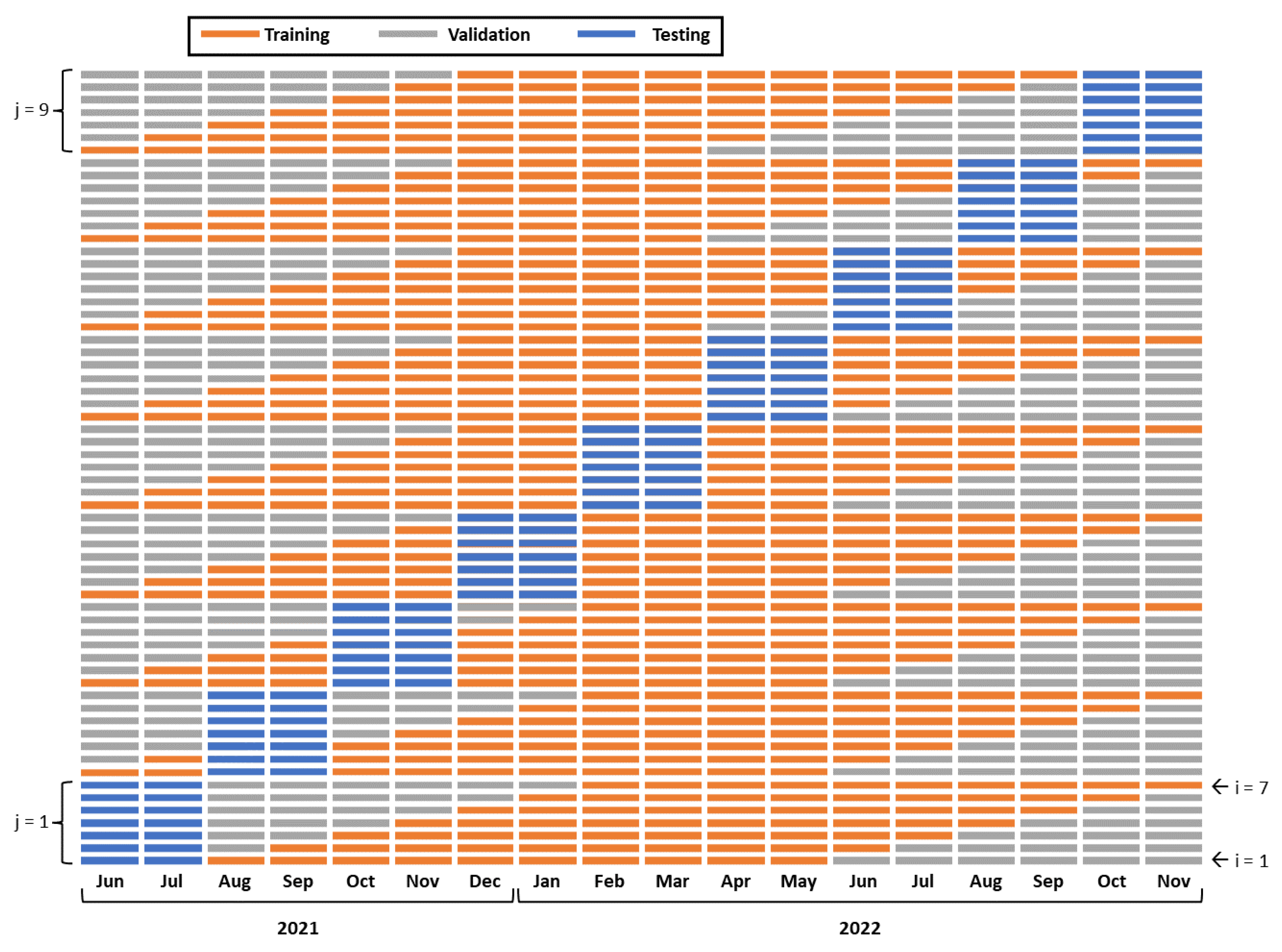
The splits were performed multiple times to obtain a k-fold cross-validation sequence. The data were split into 18 equal subsets, which approximately correspond to the 18 calendar months present in the time period (from June 2021 to December 2022). In order to create the test subsets, we started by selecting the first two months of the 18-month period and then moved on to the successive non-overlapping two-month subsets until we reached the end of the period. This resulted in 9 distinct test subsets. For each test split iteration, setting aside the 2 test months, there was a second validation split-sequence: from the remaining 16 months, 10 months were selected for training and 6 months were selected for validation. To create a statistical variation of the model and to allow for an ensemble averaging of the results, multiple validation split sequences were created as follows: the training data were moved forward by one month in each iteration and the remaining data were selected for validation. This way, 7 different training/validation split sequences can be created for a single test split-sequence. The split sequences are shown in Figure 2. An important property of our data splitting is that for a given selection of the testing period, each of the 7 training sets only includes distinct months (no month is repeated in a given training set). Following these rules, we have a total of 63 (9 × 7) model runs. The final result is derived from these models as follows: for each 2-month testing period, the output is predicted only for the corresponding I = 7 ensemble model members. Finally, the  J = 9 test outputs are concatenated to form a 7-member ensemble of 18-month test sequences. This ensemble will be used to assess the performance of the model. The average Y ¯ of the ensemble members Y ^ i is the model’s output:
Y ¯ = 1 I i = 1 I Y ^ i
This model output is compared to the ground truth Y ˜ (WRF simulation) to estimate model accuracy while the model uncertainty is derived from the dispersion of the ensemble members.

2.6. Statistical Downscaling Models

2.6.1. Linear Regression Model

Previous statistical downscaling studies by Baño-Medina et al. [33] and Hernanz et al. [70] have used a multiple linear regression (MLR) model for temperature prediction. In this study, such a model is used as a benchmark to assess the performance of our deep-learning downscaling approach. Initially, the model is used to conduct a feature selection investigation whereby the most significant lagged inputs are identified.
Wilby et al. [71] developed a model based on multiple regression for statistical downscaling of data from GCMs onto site-specific daily surface weather conditions. The main challenge was to choose the appropriate predictor variables—which vary spatially and temporally—since they largely impact the downscaled results. Therefore, only statistically significant predictors were used by the model in their study. Similarly, in this study, the inputs and outputs are composed of spatio-temporal data. Therefore, a feature selection routine is performed as a preprocessing step to reduce the dimensionality of the input data. Note that in our case, the input data only consist of one variable: LST. In order to estimate the significant time lags (features), a preliminary linear regression model with sequential feature selection capability (using the mlxtend.feature_selection package developed by Raschka [72]) was implemented.
For the purpose of feature selection, we used a single linear regression model for the entire input dataset. Therefore, the input data were flattened in the spatial dimensions so that only the time dimension persists. For each LST input pixel, the current time and twelve previous time lags were evaluated for the prediction of the near-surface air temperature in the output pixel. Both forward and backward feature selection procedures were carried out. In the forward selection procedure, candidate time lags were added one by one in such a way that the best R 2 score was obtained after each addition. In the backward selection procedure, we started by including all 12 time lags in the model, and then features were removed one by one, such that the best R 2 persisted after each elimination. In both cases, the procedure was repeated until the stopping criteria for R 2 (<0.05%) suggested by Wilks [73] was reached. This means that the features were added/removed in forward/backward feature selection, respectively, until the change in R 2 was less than 0.05 %. This resulted in retaining seven features in both cases. The retained time lags were ( 12 , 9 , 6 , 5 , 2 , 1 , 0) for forward selection, and ( 12 , 7 , 6 , 5 , 2 , 1 , 0) for backward selection. The significant time lags were the same except for one. In the forward selection iteration, the −9 time lag was the last feature that was selected before the procedure was stopped. In the backward selection procedure, the  7 time lag was deemed more important. However, while the forward selection method showed that the 7 time lag remained highly significant—even though it was finally not retained because of the stopping criterion—the backward selection method did not deem the −9 time lag to be of high significance. Therefore, the lag 7 was included in this study instead of the lag 9 . Finally, the ( 12 , 7 , 6 , 5 , 2 , 1 , 0) time lags were used for training the benchmark model.
Standard linear regression models, when used for spatial data analysis, suffer from the high dimensionality of the input data. Therefore, MLR models were trained (a separate model is used for each pixel) similar to Baño-Medina et al. [33]. This resulted in 2304 (48 × 48) LR models, where each model uses only the 7 previously identified time lags as input.
In addition to this, the ridge regularization (L2 penalty) method, similar to Hernanz et al. [70], was implemented (using the scikit-learn Python package) to avoid over-fitting and improve generalization. The lsqr solver was used since it uses the regularized least-squares routine, and it is relatively fast. The benchmark model used the training-validation-test data splits defined previously (Figure 2). For each training/validation split, the  α parameter was obtained using scipy’s “minimize scalar” constrained optimization algorithm “bounded”. This algorithm finds the optimum α parameter within the specified bounds (in our case, between 0 and 10) that minimizes the mean square error on the validation dataset.

2.6.2. Deep Learning Model

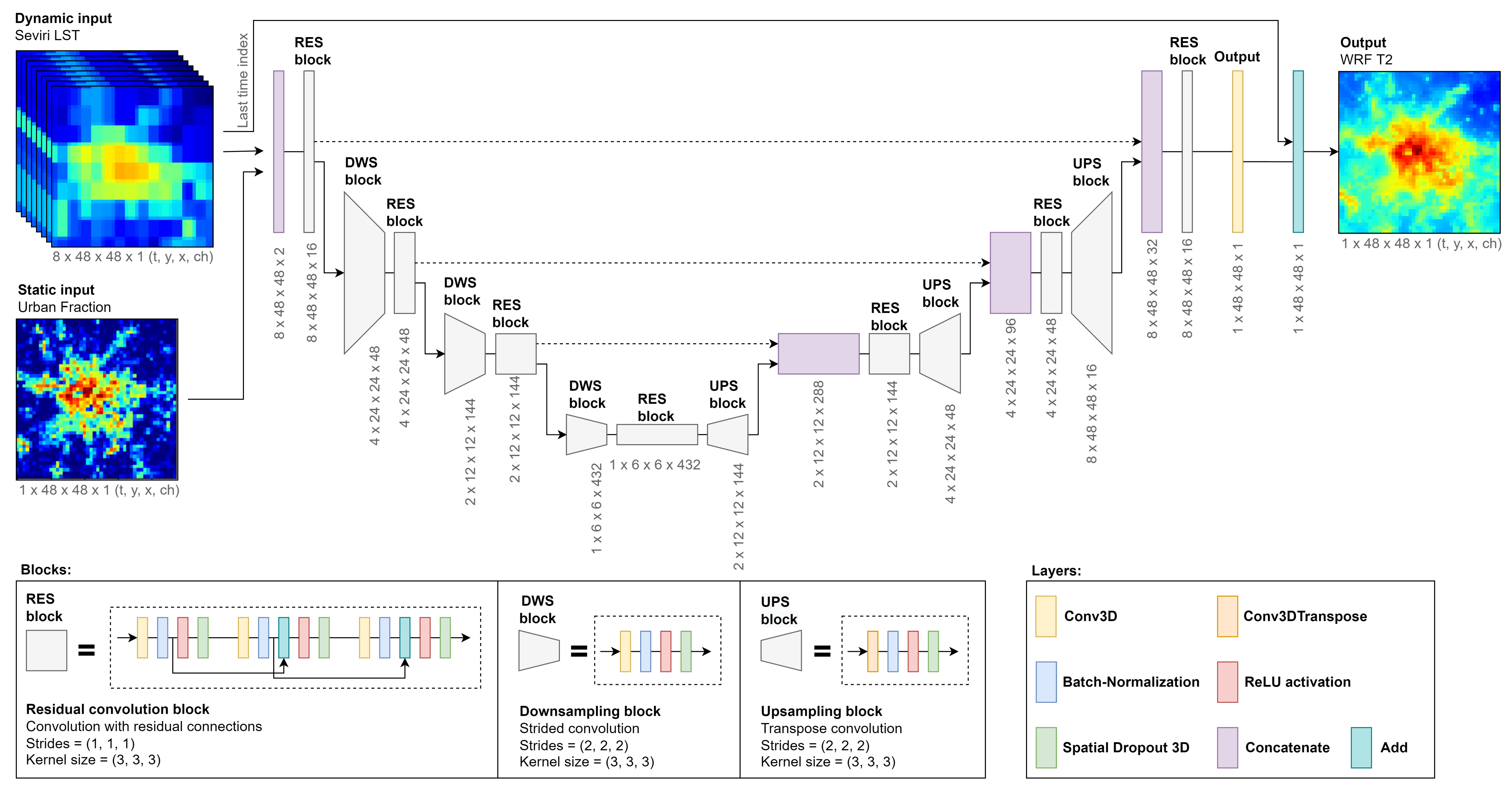
Our deep learning (DL) downscaling model was based on the U-Net structure that was originally proposed by Ronneberger et al. [11] for image segmentation. The variant we implement is mostly inspired by the research on downscaling temperature and wind fields by Höhlein et al. [4], Serifi et al. [35] and Gomez Gonzalez [49]. We tested many different model types and selected the architecture that performed best for the given task of statistical downscaling from coarse resolution LST to fine resolution WRF near-surface air temperature. The model was implemented using Tensorflow [74]. An illustration of the model is shown in Figure 3.
At each time step, the model uses several time steps of the 2D input data (SEVIRI LST) as well as an additional static 2D input (urban fraction) to predict the current 2D map of the output (WRF near-surface temperature). The dynamic input data are LST at a spatial resolution of about 3 km × 5 km; however, as described in Section 2.4, the data are already on the target grid resolution after conservative interpolation. As a result, both the input and output data are on a grid of 48 × 48 grid pixels at a resolution of 1 km × 1 km.
The selection of input and output time steps (windowing operation) was described in Section 2.4. In the last Section 2.6.1, it was pointed out that a sequence of 7 time steps (current and previous lags) of the input was sufficient to optimize the linear regression model. However, for our DL model, and especially the U-Net structure, it is beneficial to have a number of time steps that can be divided by 8 and that have an equal step distance. The reason is that the U-Net we propose reduces the dimensions of both space and time, where the dimensions need to be equally sampled and divisible by two for each U-Net level. Therefore, we modified the input sequence to include the following 8 time steps (−14, −12, −10, −8, −6, −4, −2, 0). This fulfills the structural requirement while at the same time being close to the lags identified by the feature selection procedure described in Section 2.6.1.
In a first layer, the dynamic and static inputs are concatenated along the channel dimension after broadcasting the static input to the dimensions of the dynamic input. The result is an input tensor with shape (t: 8, y: 48, x: 48, c h : 2), where t is the time, y and x are the grid dimensions of the WRF coordinate system, and c h is the “channel” dimension that becomes the dimension of feature-maps in the subsequent convolutional layers. After the concatenation layer, a first residual block is used to create an initial set of 16 feature maps. In each level of the encoder part of the U-Net, a downsampling (DWS) block is followed by a residual convolution (RES) block. The downsampling block includes a strided convolution layer with strides (2, 2, 2), which results in a reduction of the t, y, and x dimensions by a factor of 2. Every residual block contains 3 convolution layers with strides (1, 1, 1) and two residual connections. In each level of the decoder part of the U-Net, an upsampling (UPS) block is followed by a concatenation of the skip connection along the channel dimension and a RES block. The upsampling block includes a transpose convolution layer with strides (2, 2, 2), which results in an increase of the t, y, and x dimensions by a factor of 2. After the decoder, an output layer creates a single high-resolution temperature map that corresponds to the last time step of the dynamic input. The output is created using a convolution layer and setting the kernel size to (1, 1, 1) and the number of feature maps to 1. Finally, the last time step of the input is added to the output, which resembles a residual connection over the whole model, i.e., the model only predicts the residual between the output and the last time step of the dynamic input.
The number of feature maps is tripled in each level of the U-Net, i.e., 48 in the first level, 144 in the second level, and 432 in the final level (often referred to as the latent state). Having a factor of three instead of two is a good compromise between the more common factor of two that is used in other studies and the factor of 8 that would be needed to preserve the total size of the 4D tensor (each U-Net level reduces the size of each of the 3D input dimensions by a factor of 2, leading to a total reduction of the input size by a factor of 8).
The optimal model activation and regularization were thoroughly investigated by testing different layer orderings with and without dropout and normalization. Our final optimized setup was as follows: every convolution layer was followed by a normalization layer, an activation layer, and a dropout layer. For normalization, we used batch-normalization, for activation, the rectified linear unit (ReLU), and for dropout, the spatial 3D dropout with a rate of 0.2, i.e., 20% of the feature maps were deactivated randomly during training. There are mixed reports of using dropout and normalization together. Höhlein et al. [4] mentioned previous research revealing performance issues when using dropout and normalization together. However, they reported that they did not encounter these issues themselves. In our case, using normalization and dropout together was the optimal configuration to prevent excessive over-fitting of the model.
We used a mixed loss function based on the mean square error (MSE), mean square gradient error (MSGE), and structural dissimilarity (DSSIM). Combining MSE and MSGE was described by Abrahamyan et al. [75] and Lu and Chen [76]. Using DSSIM in addition to MAE or MSE was investigated by Gomez Gonzalez [49]. After testing different weights, we found the following combination to perform best: 50% MSE, 10% MSGE, and 40% DSSIM.
To train the model, we used the ADAM optimizer with a learning rate of 3 × 10⁻⁴. The input data were fed into the model using a data generator. The data generator prepared the data in batches of 5 days (120 samples) from the training set that contained a total number of 7300 samples. The training data were shuffled initially and then again after each epoch. The validation set, which included 4379 samples, was used for early stopping and selecting the best weights found during training. The optimization continued until no improvement of the validation loss by at least 1 × 10⁻³ could be observed in the last 20 epochs. The early stopping algorithm was configured to always preserve the weights of that epoch having the lowest validation loss. This way, even when the model starts over-fitting, the final model weights are the ones for which the model performed optimally on the validation set. The model typically needed between 100 and 150 epochs to converge.

3. Results and Discussion

3.1. Input Uncertainty

The DL model implicitly assumes that the error in the input LST data, while possibly spatially differentiated, is temporally consistent. Problems can arise if the input error also varies in time, especially if said temporal variations are not the same for land-cover types. In other words, further examination of the daily and seasonal fluctuations of the error of the satellite sensor is required.
The ability of the remote sensor to reproduce the actual land surface temperature is typically characterized by the bias and the RMSE between remotely sensed LST and in situ-measured LST. Trigo et al. [77] analyzed error data for SEVIRI and, specifically, the LSA-SAF LST product based on measurements collected at the Evora (Portugal) rural validation station in 2005–2006. They reported that the bias was generally positive in the day-time by about 2  ° C on average. As explained by Bechtel et al. [60], since SEVIRI views Europe from the south, the day-time warm bias is likely to be even higher in urban areas where south-oriented vertical surfaces are generally warmer than (unseen) north-oriented ones. Night-time SEVIRI values presented a negative bias ranging from −0.4  ° C to −2.5  ° C.
The day-time RMSE in September (∼summer) was highest at 4.9  ° C. January (∼winter) was more accurate with a day-time RMSE of 2.7  ° C. November (∼fall) was even more accurate with a day-time RMSE of 1.4  ° C. Finally, in May (∼spring), the day-time RMSE was lowest at 1.0  ° C. The night-time RMSE was 2.9  ° C in September, 1.9  ° C in November, 0.90  ° C in January and 2.4  ° C in May. In summary, according to the results of this limited study, the most accurate LST values corresponded to winter night-time and spring day-time with RMSEs in the range 0.90–1.0  ° C. Fall had intermediate accuracy with RMSE in the range 1.4–1.9  ° C. Winter day-time and spring night-time were even less accurate with RMSE in the range 2.4–2.9 ° C. Finally, the least accurate period was summer day-time with an RMSE of 4.9  ° C.
This complex time and land-cover dependency of the SEVIRI sensor error accounts for some of the intractable aspects of the variability of the overall model output error that we will analyze in the following sections.

3.2. Overall Model Error and Accuracy Metrics

The epistemic uncertainty can be analyzed by calculating the standard deviation over all I = 7 members of the ensemble of model predictions Y ^ i ( t , n , m ) where t [ 1 , , T ] , n [ 1 , , N ] and m [ 1 , , M ] are the indices of, respectively, the time coordinate, the x-coordinate, and the y-coordinate. Note that each ensemble member is the concatenation of J = 9 test outputs and spans a full 18-month period. First, we calculate the ensemble average Y ¯ ( t , n , m ) . Then, the overall standard deviation of the DL model can be calculated as follows:
σ ^ = 1 I T N M 1 i = 1 I t = 1 T n = 1 N m = 1 M [ Y ^ i ( t , n , m ) Y ¯ ( t , n , m ) ] 2
The following overall error metrics were calculated over all selected data points, where Y ˜ ( t , n , m ) denotes the ground truth:
  • Mean bias error:
    MBE = 1 T N M t = 1 T n = 1 N m = 1 M [ Y ¯ ( t , n , m ) Y ˜ ( t , n , m ) ]
  • Mean absolute error:
    MAE = 1 T N M t = 1 T n = 1 N m = 1 M | Y ¯ ( t , n , m ) Y ˜ ( t , n , m ) |
  • Root mean square error:
    RMSE = 1 T N M t = 1 T n = 1 N m = 1 M [ Y ¯ ( t , n , m ) Y ˜ ( t , n , m ) ] 2
  • R-squared:
    R 2 = 1 t = 1 T n = 1 N m = 1 M [ Y ¯ ( t , n , m ) Y ˜ ( t , n , m ) ] 2 t = 1 T n = 1 N m = 1 M [ Y ˜ ( t , n , m ) 1 T N M t = 1 T n = 1 N m = 1 M Y ˜ ( t , n , m ) ] 2
  • Peak signal-to-noise ratio:
    PSNR = 20 log 10 max t , n , m { Y ˜ ( t , n , m ) } min t , n , m { Y ˜ ( t , n , m ) } RMSE
  • P ( AE < ° C), the probability of getting an absolute error (AE) that is smaller than 2  ° C:
    AE ( t , n , m ) = | Y ¯ ( t , n , m ) Y ˜ ( t , n , m ) |
    AE 2 ( t , n , m ) = 1 , if AE ( t , n , m ) < 2 0 , otherwise
    P ( AE < 2 ° C ) = 1 T N M t = 1 T n = 1 N m = 1 M AE 2 ( t , n , m )
The structural similarity (SSIM) was calculated using the function tf.image.ssim in Tensorflow [74] following Wang et al. [78]. The structural similarity is defined for a 2D-array and it is calculated in a convolutional fashion using an 11 by 11 Kernel. Also, the SSIM calculation assumes positive values and requires the dynamic range of the data. Therefore, we used the global minimum and maximum values to calculate the dynamic range for the PSNR, see Equation (8). Before calling the function to calculate the SSIM, the global minimum was subtracted to offset the data so that all values were positive.
To visualize the model errors in 2D maps as well as box-plots for spatial variability, the following metrics were only averaged over time to retain the space dimensions:
  • Mean bias error map:
    MBE ( n , m ) = 1 T t = 1 T [ Y ¯ ( t , n , m ) Y ˜ ( t , n , m ) ]
  • Mean absolute error map:
    MAE ( n , m ) = 1 T t = 1 T | Y ¯ ( t , n , m ) Y ˜ ( t , n , m ) |
  • Root Mean Square Error map:
    RMSE ( n , m ) = 1 T t = 1 T [ Y ¯ ( t , n , m ) Y ˜ ( t , n , m ) ] 2

3.3. Model Evaluation

As described in Section 2.4, the models were run in a cross-validation fashion, which results in a 7-member test output ensemble (concatenation of the results for each test subset) spanning a period of 18 months. The final output is the average of the ensemble.
The overall standard deviation of the DL model output was determined following Equation (3), to be σ ^ = 0.479 ° C or approximately 0.50 ° C. Accordingly, assuming that the epistemic error is normally distributed, a 95% confidence interval around the ensemble average would correspond to the range Y ¯ ± 1.0 ° C, while a 99% confidence interval would correspond to the range Y ¯ ± 1.5 ° C.
To evaluate the error of the DL model compared to the benchmark approach, we analyzed the data over the last 12 months of the 18-month period used in training, i.e., from 21 December 2021 until 21 December 2022. The repeated seasons occurring in the first calendar year of the 18-month period (i.e., summer 2021 and fall 2021) were left out of this averaging exercise in order to avoid skewing the metrics.
The overall metrics used in this evaluation were calculated using all data points of the predicted model output and the ground truth over the selected 12-month period. The results are given in Table 2.
Both the benchmark MLR model and the U-Net model predicted the output sufficiently well. With the exception of the model bias, the DL model was superior on all metrics. In particular, MAE, RMSE, and all the 98th percentile (warmest 2%) model errors were clearly smaller than the benchmark. In addition, P( AE < 2 ° C), the probability of the absolute error being less than 2 degrees was 7% higher than the benchmark.
A major difference between the models is that for the benchmark implementation, a separate linear regression model was estimated for each grid pixel. The model was, therefore, fully fitted to each pair of input/output pixels which, unsurprisingly, leads to quite accurate predictions. However, given that it is a linear model, it is unable to predict nonlinearities. The U-Net model architecture is much more complex and includes the correlation of temperature to an urban fraction. Therefore, it is expected to better generalize to other regions and domain sizes. However, these potential advantages of the DL model cannot be seen in this comparison where the increase in accuracy compared to the benchmark may seem moderate (although it is quite significant for the 98th percentile).
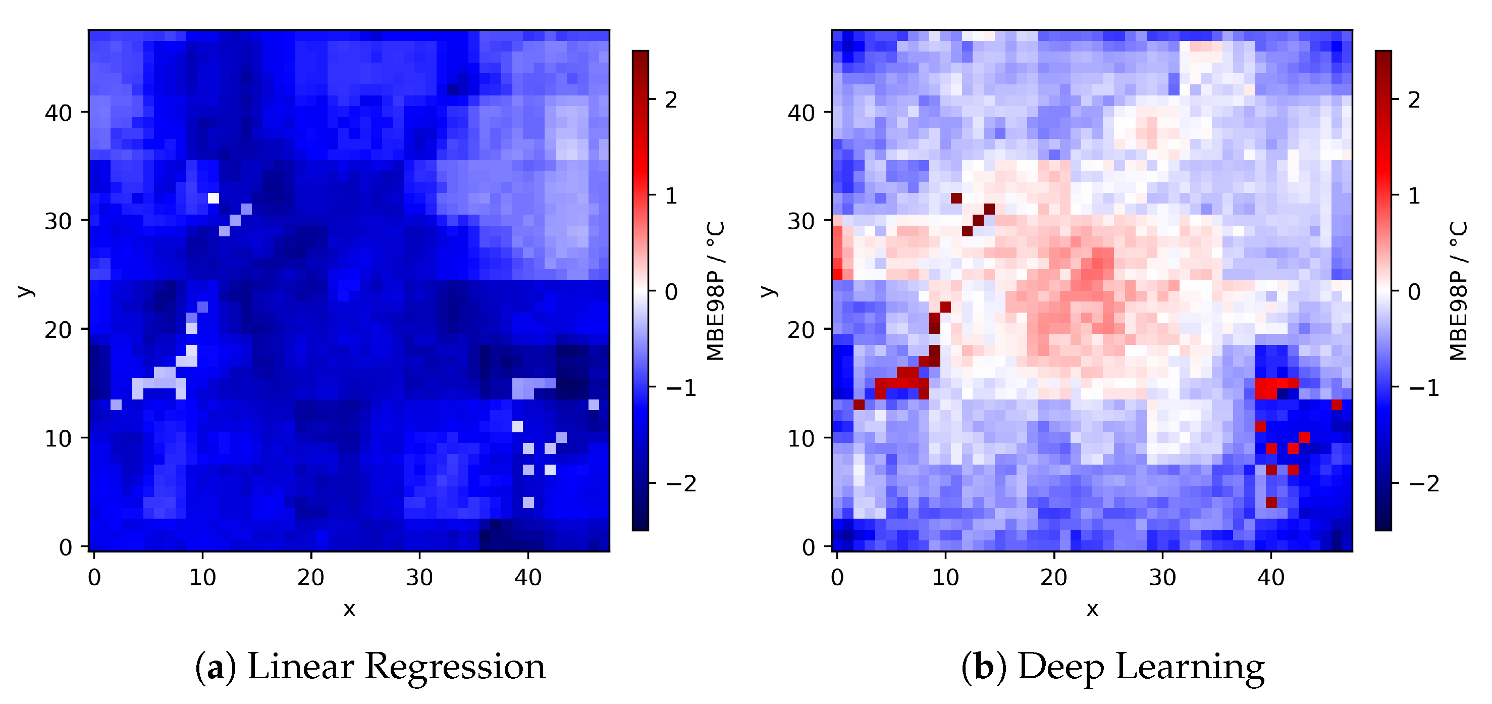
To characterize and compare the DL model’s ability to capture the spatial variability of the prediction for extreme hot weather, the 2 % warmest time steps were averaged. First, all predicted space-time data points over the 12-month period were analyzed and the hottest 2% were selected. Then, for the selected data points, the corresponding 2D maps were averaged along the time dimension. The outcome of this exercise for MBE98P is shown in Figure 4. While the linear regression model mostly under-predicts the temperature by more than 1 ° C, the pixel-by-pixel average bias of the DL model is lower and better distributed around zero: urban pixels showed over-prediction, while rural pixels were mostly under-predicted. This general urban over-prediction was consistent with the comment made earlier about the fact that, in urban areas, the LST sensor sees mostly warmer south-oriented walls. In other words, in such areas, the SEVIRI-measured LST is higher than the true LST.
Both models show stark discontinuity over some rural pixels to the west and the south-east of the domain. These pixels correspond to water surfaces and their immediate surroundings. While the linear regression model shows relatively good accuracy over these pixels, the DL model over-predicts the near-surface temperature above/near water by close to 2 ° C. This underlines one inherent advantage of the MLR approach, where each pixel is predicted by its own model, whereas the more compact convolutional model is, by construction, less adept at modeling very localized and discontinuous phenomena. Nonetheless, the DL model’s output is generally more accurate and more spatially homogeneous compared to the linear regression model.

3.4. Seasonal Variability of the Model Performance

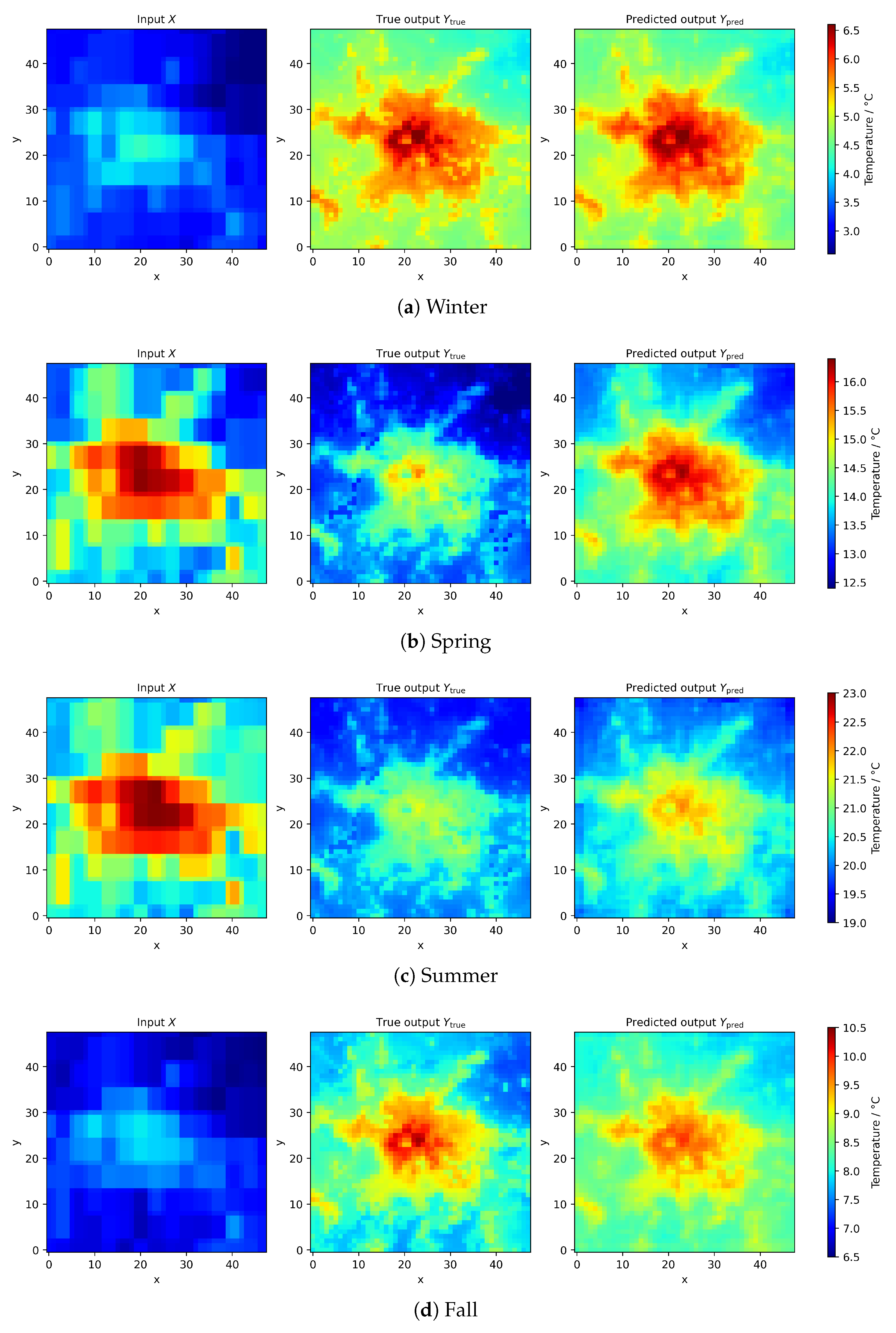
To capture the seasonality of the DL model’s performance, we analyzed the data over the four seasons of the previously analyzed 12-month period: (1) Winter from 21 December 2021 until 21 March 2022, (2) Spring from 21 March 2022 until 21 June 2022, (3) Summer from 21 June 2022 until 21 September 2022, (4) Fall from 21 September 2022 until 21 December 2022. The model predictions of temperature during different seasons are illustrated in Figure 5. Note that the color scale is, necessarily, different for each season. However, to facilitate comparison, the range is the same in each case: 4 ° C.
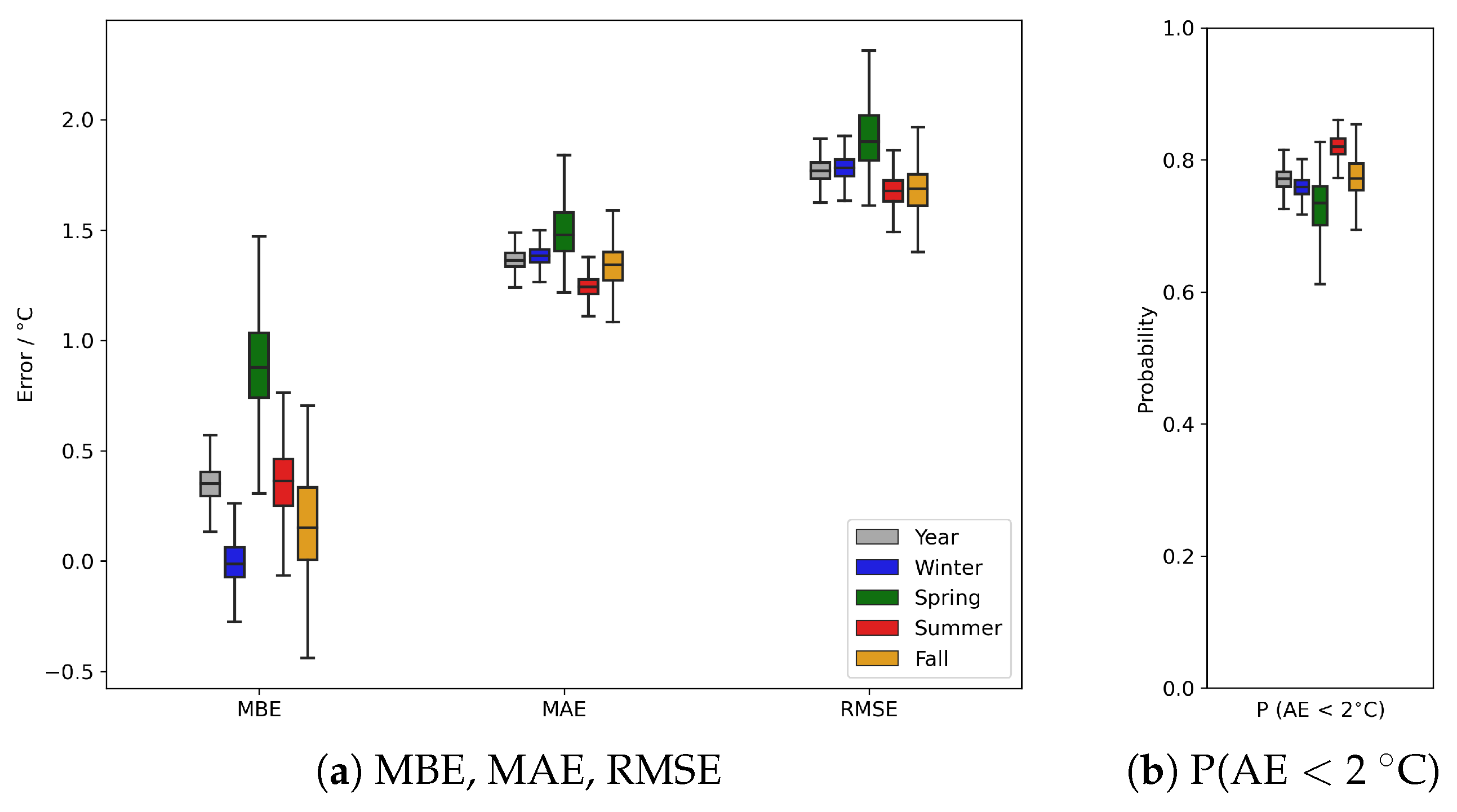
According to Figure 5, over most of the year (winter, spring, summer), the urban near-surface air temperature was over-predicted, while under-prediction occurred in rural areas. In fall, on the other hand, the temperature in the urban center was slightly under-predicted while over-prediction was detected in the peripheral rural region. The bias of the DL model in winter was generally small and slightly negative for most pixels. In the other seasons, the model over-predicted on average. The most challenging season for the model seemed to be spring and, to a lesser extent, summer.
The average seasonal metrics of the DL model are provided in Table 3. For each metric, the best-performing seasonal value is shown in bold font. According to these overall metrics, winter had the lowest bias and the highest SSIM. The fall season had the second-best MBE, the best PSNR, and the best RMSE. Summer had the best MAE, the best P( AE < 2 ° C), and the same RMSE as fall. Finally, spring was worse than other seasons on all metrics except R 2 .
We also provide, in Figure 6, the box plots showing the spatial variation of seasonal performance metrics over the study area, time-averaged for different seasons. The center-line corresponds to the median of the distribution. The box extremes correspond to the quantile values (25th and 75th percentile) of the distribution. The extreme lines correspond to maximum and minimum values in the distribution calculated using quantiles and the inter-quantile range. All the metrics indicate that the spring season error had the highest variability in comparison to other seasons. Spring was also the worst performing season on all average metrics, as was previously seen in Table 3. Fall metrics showed the highest dispersion after spring. That being said, in terms of average metrics, it was significantly better than spring. Overall, winter has the lowest MBE but performs worse than summer and fall when it comes to MAE and RMSE. Summer has the lowest MAE and RMSE, but its MBE is higher than winter and fall. The model generally over-predicts (positive average bias) in spring, summer, and fall.
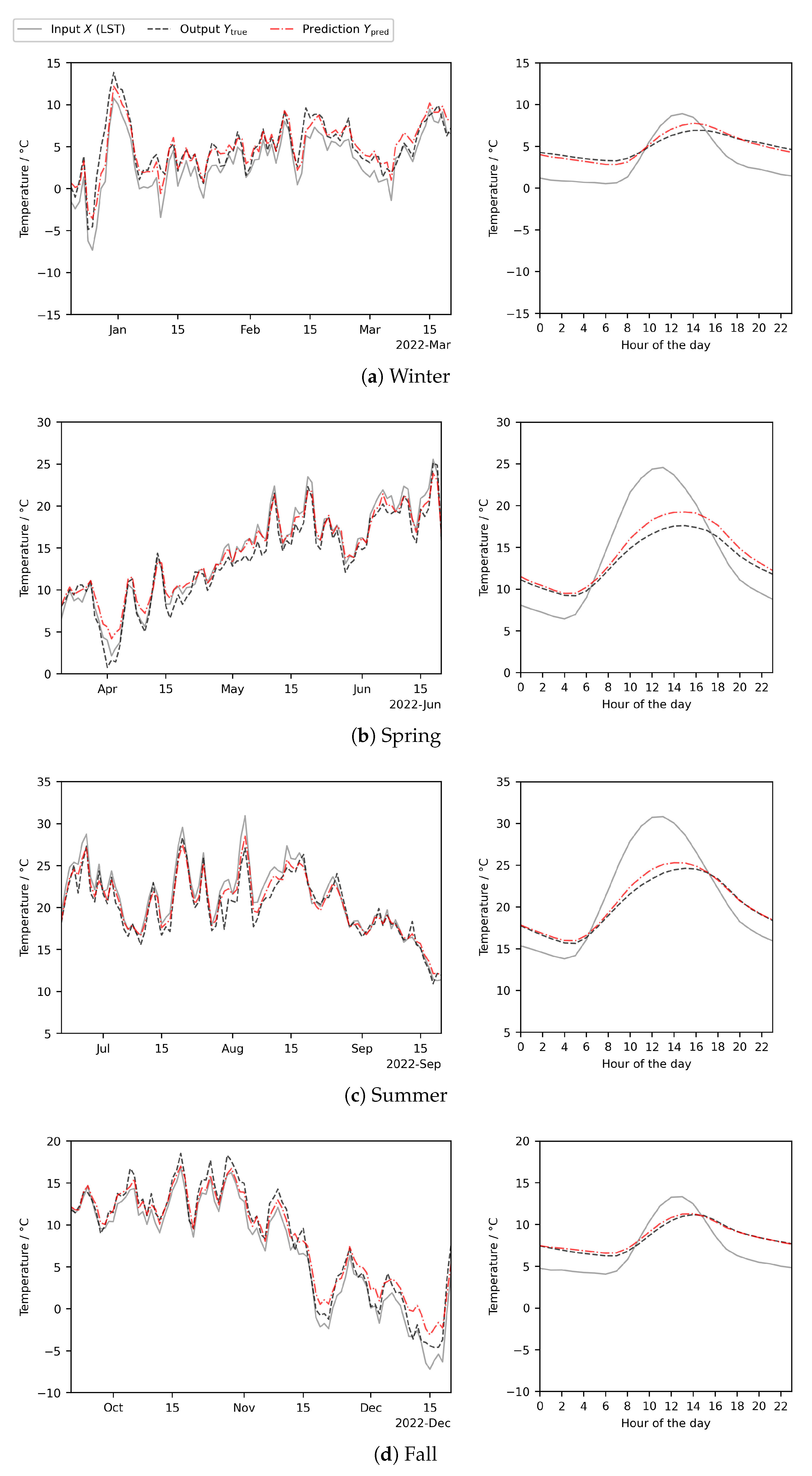
The time series of daily average values, as well as the average daily profiles of hourly values, for different seasons are illustrated in Figure 7. As can be seen on this figure, the daily average values are quite accurate throughout the year. In spring, fall, and summer, on those days when the average daily temperature fell suddenly in comparison to the previous trend—presumably due to cloudy/rainy days for which LST data had to be gap-filled—the model over-predicted, sometimes significantly. As can be seen on the average daily profiles, the over-prediction occurred mostly during day-time while the night-time prediction is quite accurate. In winter, slight diurnal over-prediction and nocturnal under-prediction co-exist and are approximately of the same magnitude. In winter and fall, the amplitude of the average day/night air temperature fluctuation was small and only slightly less than the corresponding LST fluctuation. Over the remainder of the year (spring and summer), the amplitude of the average day/night air temperature fluctuation was higher than in fall and winter. In addition, in spring and summer, day-time LST tended to be much higher than the air temperature: the maximum average discrepancy exceeded +6 ° C. The night-time discrepancy was generally smaller and more stable over the course of the night. It was nearly the same for all seasons, of the order of −3 ° C.

3.5. Generalizability of the Model

To test the generalizability of the model, we apply the trained model to four different domains on the four cardinal corners of the primary region of interest (ROI). These secondary ROIs have the same size as the primary ROI, i.e., 48 × 48 pixels. They all share their innermost quadrant (1/4th of the total domain area) with the primary ROI, while the three other quadrants were unseen by the trained model. As an example, the south-western secondary domain is shown in Figure 1.
The annual metrics for each of these secondary ROIs are shown in Table 4, where the core (primary) ROI metrics are also repeated to facilitate comparison. The deterioration is highest for the prediction bias. It was less accurate (less than 15% increase) when it came to MAE and RMSE. In all cases, the RMSE remained below 2 ° C and P( AE < 2 ° C) above 0.70. PSNR and SSIM were only slightly affected, with deterioration well below 5%.

4. Conclusions and Outlook

4.1. Conclusions

In this study, we develop and evaluate a method to emulate the Weather Research and Forecasting (WRF) model in a nowcasting application. The proposed deep learning model predicts the current high-resolution ( 1 × 1 km 2 pixels) near-surface air temperature from current and past low-resolution land surface temperatures measured by the SEVIRI sensor. The spatial resolution of the input is downscaled by about a factor of four. A modified U-Net architecture was derived that implements a novel space-time approach where multiple time steps are fed into the model through 3D convolution layers. Besides LST, the model uses the urban density as additional static input. The performance of the proposed deep learning model was compared to that of a pixel-by-pixel multiple linear regression model using ridge regularization (benchmark). The intention is to apply the trained model to nowcasting or, perhaps, short-term forecasting (e.g., next 6–24 h) in future work. For that reason, it is desirable that the model is driven solely by the LST feed, which is available in quasi-real-time.
The model was trained, validated, and tested on a 48 × 48 km 2 domainbreak, including the city of Berlin and extending slightly into the rural landscape around the city. Here, 18 months of hourly input/output data were used. An original training/validation/testing split of the total period was derived which avoids repeated calendar months in the 10-month training period over all the validation folds. In addition, for each of the nine test splits, there were seven training/validation splits, resulting in an ensemble of seven concatenated test outputs. The average of the ensemble was used as the model output while the dispersion of the ensemble elements was used to approximate the epistemic uncertainty of the model.
The error of the DL model was compared to the benchmark MLR approach. With the exception of the model bias, the DL model was superior on all metrics. The superiority was even more pronounced for the 2% warmest hours of the evaluation period. Generally, urban pixels show over-prediction while rural pixels are mostly under-predicted. On the other hand, the DL model strongly over-predicts the air temperature over water surface pixels. Nonetheless, the DL model’s output is generally more accurate and more spatially homogeneous compared to the benchmark. A significant proportion of the model’s inaccuracy can be attributed to the largely intractable SEVIRI sensor measurement error which is highly variable in time and space. The most challenging season for the model is spring and, to a lesser extent, summer. Overall, winter has the lowest MBE but performs worse than summer and fall when it comes to MAE and RMSE. Summer has the lowest MAE and RMSE, but its MBE is higher than winter and fall. The model generally over-predicts in spring, summer, and fall. In spring, fall, and summer, the model over-predicts during day-time, while the night-time prediction is quite accurate. In winter, slight diurnal over-prediction and nocturnal under-prediction co-exist and are approximately the same magnitude.
The mostly positive bias results from unpredictable seasonal/annual discrepancies that naturally exist between the input–output behavior in the training data and the input–output behavior in the corresponding test data. It is difficult to address this bias directly. The best approach would be to conduct the analysis over a significantly longer period (e.g., 5–10 years instead of 18 months). Given that we use hourly data, this would require significant computation effort, both on the WRF side and on the ML side. It is, nonetheless, one of the future improvement tracks that are envisioned.
The generalizability of the model was tested by applying the trained model to four different domains on the four corners of the primary region of interest (ROI). The deterioration in comparison to the primary ROI is highest for the prediction bias. It is less accurate when it comes to MAE and RMSE (less than 15% increase). In all cases, the RMSE remains below 2 ° C and P( AE < 2 ° C) above 0.70. PSNR and SSIM are only slightly affected, with deterioration well below 5%.
The study sets forth the following contributions:
  • The proposed application is original: nowcasting of high-resolution near-surface air temperature (WRF emulation) in near real-time conditions using as input high-frequency but low-resolution SEVIRI LST images;
  • The proposed deep learning model implements a novel space-time approach, where multiple time steps are fed into the model through 3D convolution layers;
  • Clear superiority of the proposed deep learning model is demonstrated based on a comprehensive set of evaluation metrics, in comparison to a finely tuned multiple linear regression benchmark;
  • Generalizability is established by applying the deep learning model to domains that were mostly unseen during training.

4.2. Outlook

Future research work will pursue the following improvement tracks:
  • Conduct the analysis over an extended period (several years) in order to reduce the bias;
  • Use a separate model for each season: The seasonal variations of the model error, presumably attributable in large part to the seasonal variability of the input error, call for a clear differentiation between the seasons;
  • Explore more effective ways to incorporate daily/seasonal patterns into the model: Fourier harmonics, etc.;
  • Investigate other deep learning model architectures: convolutional LSTM, GAN, etc.;
  • Include additional regularizers into the loss function: Ability to enforce physical conservation laws would be ideal in this context;
  • Systematically optimize hyper-parameters: For instance, the regularization coefficients in the loss function;
  • Use, as input to the deep learning model, further gridded static data maps to characterize anthropogenic heat, topography, land cover, and urban morphology (to the extent such data is also taken into account in the WRF simulation): For instance, road density (e.g., from OpenStreetMap), population density, average building height, roughness length, land/water mask, NDVI (Normalized Difference Vegetation Index), terrain elevation, etc.;
  • Add LST data from non-geostationary satellites: MODIS, ASTER, etc.;
  • Apply to short-term forecasting: with minimal modifications, use the model to forecast near-surface air temperature a few hours ahead; this forward-looking capability will enable us to cover the short latency that currently exists in the availability of the SEVIRI LST data.

Author Contributions

Conceptualization, A.A. and J.V.; methodology, J.V., A.A. and G.C.; software, J.V. and G.C.; validation, J.V., G.C. and A.A.; data curation, J.V. and G.C.; writing—original draft preparation, A.A., J.V. and G.C.; writing—review and editing, A.A. and J.V.; visualization, J.V. and G.C.; supervision, A.A.; funding acquisition, A.A. All authors have read and agreed to the published version of the manuscript.

Funding

This research was supported by Fraunhofer Internal Programs under Grant No. Attract 003-695033.

Data Availability Statement

The data presented in this study are available on request from the corresponding author.

Conflicts of Interest

The authors declare no conflict of interest. The funders had no role in the design of the study; in the collection, analyses, or interpretation of data; in the writing of the manuscript; or in the decision to publish the results.

References

  1. Masson-Delmotte, V.; Zhai, P.; Pirani, A. Climate Change 2021: The Physical Science Basis: Summary for Policymakers: Working Group I Contribution to the Sixth Assessment Report of the Intergovernmental Panel on Climate Change; IPCC: Geneva, Switzerland, 2021. [Google Scholar]
  2. Fiedler, T.; Pitman, A.J.; Mackenzie, K.; Wood, N.; Jakob, C.; Perkins-Kirkpatrick, S.E. Business risk and the emergence of climate analytics. Nat. Clim. Chang. 2021, 11, 87–94. [Google Scholar] [CrossRef]
  3. Feser, F.; Rockel, B.; von Storch, H.; Winterfeldt, J.; Zahn, M. Regional Climate Models Add Value to Global Model Data: A Review and Selected Examples. Bull. Am. Meteorol. Soc. 2011, 92, 1181–1192. [Google Scholar] [CrossRef]
  4. Höhlein, K.; Kern, M.; Hewson, T.; Westermann, R. A comparative study of convolutional neural network models for wind field downscaling. Meteorol. Appl. 2020, 27, e1961. [Google Scholar] [CrossRef]
  5. Deser, C. Certain Uncertainty: The Role of Internal Climate Variability in Projections of Regional Climate Change and Risk Management. Earth’s Future 2020, 8, e2020EF001854. [Google Scholar] [CrossRef]
  6. Wilby, R.; Wigley, T. Downscaling general circulation model output: A review of methods and limitations. Prog. Phys. Geogr. Earth Environ. 1997, 21, 530–548. [Google Scholar] [CrossRef]
  7. Chandler, R.E. On the use of generalized linear models for interpreting climate variability. Environmetrics 2005, 16, 699–715. [Google Scholar] [CrossRef]
  8. Reichstein, M.; Camps-Valls, G.; Stevens, B.; Jung, M.; Denzler, J.; Carvalhais, N.; Prabhat, F. Deep learning and process understanding for data-driven Earth system science. Nature 2019, 566, 195–204. [Google Scholar] [CrossRef]
  9. Goodfellow, I.; Bengio, Y.; Courville, A. Deep Learning; MIT Press: Cambridge, MA, USA, 2016. [Google Scholar]
  10. Rampal, N.; Gibson, P.B.; Sood, A.; Stuart, S.; Fauchereau, N.C.; Brandolino, C.; Noll, B.; Meyers, T. High-resolution downscaling with interpretable deep learning: Rainfall extremes over New Zealand. Weather Clim. Extrem. 2022, 38, 100525. [Google Scholar] [CrossRef]
  11. Ronneberger, O.; Fischer, P.; Brox, T. U-Net: Convolutional Networks for Biomedical Image Segmentation. arXiv 2015, arXiv:1505.04597. [Google Scholar]
  12. Dong, C.; Loy, C.C.; He, K.; Tang, X. Image Super-Resolution Using Deep Convolutional Networks. IEEE Trans. Pattern Anal. Mach. Intell. 2016, 38, 295–307. [Google Scholar] [CrossRef]
  13. Yang, W.; Zhang, X.; Tian, Y.; Wang, W.; Xue, J.H. Deep Learning for Single Image Super-Resolution: A Brief Review. IEEE Trans. Multimed. 2019, 21, 3106–3121. [Google Scholar] [CrossRef]
  14. Vandal, T.; Kodra, E.; Ganguly, S.; Michaelis, A.; Nemani, R.; Ganguly, A.R. DeepSD: Generating High Resolution Climate Change Projections through Single Image Super-Resolution. In Proceedings of the 23rd ACM SIGKDD International Conference on Knowledge Discovery and Data Mining, Halifax, NS, Canada, 13–17 August 2017; pp. 1663–1672. [Google Scholar] [CrossRef]
  15. Baño-Medina, J.; Manzanas, R.; Gutiérrez, J.M. On the suitability of deep convolutional neural networks for continental-wide downscaling of climate change projections. Clim. Dyn. 2021, 57, 2941–2951. [Google Scholar] [CrossRef]
  16. Vaughan, A.; Tebbutt, W.; Hosking, J.S.; Turner, R.E. Convolutional conditional neural processes for local climate downscaling. Geosci. Model Dev. 2022, 15, 251–268. [Google Scholar] [CrossRef]
  17. Leinonen, J.; Nerini, D.; Berne, A. Stochastic Super-Resolution for Downscaling Time-Evolving Atmospheric Fields With a Generative Adversarial Network. IEEE Trans. Geosci. Remote Sens. 2021, 59, 7211–7223. [Google Scholar] [CrossRef]
  18. Watson-Parris, D. Machine learning for weather and climate are worlds apart. Philos. Trans. R. Soc. A Math. Phys. Eng. Sci. 2021, 379, 20200098. [Google Scholar] [CrossRef]
  19. Gal, Y.; Ghahramani, Z. Dropout as a Bayesian Approximation: Representing Model Uncertainty in Deep Learning. In Proceedings of the 33rd International Conference on Machine Learning, New York, NY, USA, 20–22 June 2016. [Google Scholar]
  20. Srivastava, N.; Hinton, G.; Krizhevsky, A.; Sutskever, I.; Salakhutdinov, R. Dropout: A Simple Way to Prevent Neural Networks from Overfitting. J. Mach. Learn. Res. 2014, 15, 1929–1958. [Google Scholar]
  21. Bihlo, A. A generative adversarial network approach to (ensemble) weather prediction. Neural Netw. 2021, 139, 1–16. [Google Scholar] [CrossRef]
  22. Lakshminarayanan, B.; Pritzel, A.; Blundell, C. Simple and Scalable Predictive Uncertainty Estimation using Deep Ensembles. arXiv 2017, arXiv:1612.01474. [Google Scholar]
  23. Neal, R.M. Bayesian Learning for Neural Networks; Lecture Notes in Statistics; Springer: New York, NY, USA, 1996; Volume 118. [Google Scholar]
  24. Graves, A. Practical Variational Inference for Neural Networks. In Proceedings of the 24th International Conference on Neural Information Processing Systems, Granada, Spain, 12–15 December 2011; Curran Associates Inc.: Red Hook, NY, USA, 2011; pp. 2348–2356. [Google Scholar]
  25. Beluch, W.H.; Genewein, T.; Nurnberger, A.; Kohler, J.M. The Power of Ensembles for Active Learning in Image Classification. In Proceedings of the 2018 IEEE/CVF Conference on Computer Vision and Pattern Recognition, Salt Lake City, UT, USA, 18–23 June 2018; pp. 9368–9377. [Google Scholar] [CrossRef]
  26. Ovadia, Y.; Fertig, E.; Ren, J.; Nado, Z.; Sculley, D.; Nowozin, S.; Dillon, J.V.; Lakshminarayanan, B.; Snoek, J. Can You Trust Your Model’s Uncertainty? Evaluating Predictive Uncertainty under Dataset Shift. In Proceedings of the 33rd International Conference on Neural Information Processing Systems, Vancouver, BC, Canada, 8–14 December 2019; Curran Associates Inc.: Red Hook, NY, USA, 2019. [Google Scholar]
  27. Gustafsson, F.K.; Danelljan, M.; Schon, T.B. Evaluating Scalable Bayesian Deep Learning Methods for Robust Computer Vision. In Proceedings of the 2020 IEEE/CVF Conference on Computer Vision and Pattern Recognition Workshops (CVPRW), Seattle, WA, USA, 14–19 June 2020; pp. 1289–1298. [Google Scholar] [CrossRef]
  28. Krogh, A.; Vedelsby, J. Neural Network Ensembles, Cross Validation and Active Learning. In Proceedings of the 7th International Conference on Neural Information Processing Systems, Denver, CO, USA, 28 November–1 December 1994; MIT Press: Cambridge, MA, USA, 1994; pp. 231–238. [Google Scholar]
  29. Ayhan, M.S.; Berens, P. Test-time Data Augmentation for Estimation of Heteroscedastic Aleatoric Uncertainty in Deep Neural Networks. In Proceedings of the International Conference on Medical Imaging with Deep Learning, Amsterdam, The Netherland, 4–6 July 2018. [Google Scholar]
  30. Gawlikowski, J.; Tassi, C.R.N.; Ali, M.; Lee, J.; Humt, M.; Feng, J.; Kruspe, A.; Triebel, R.; Jung, P.; Roscher, R.; et al. A Survey of Uncertainty in Deep Neural Networks. arXiv 2022, arXiv:2107.03342. [Google Scholar] [CrossRef]
  31. Wang, G.; Li, W.; Aertsen, M.; Deprest, J.; Ourselin, S.; Vercauteren, T. Aleatoric uncertainty estimation with test-time augmentation for medical image segmentation with convolutional neural networks. Neurocomputing 2019, 338, 34–45. [Google Scholar] [CrossRef]
  32. Vandal, T.; Kodra, E.; Ganguly, A.R. Intercomparison of machine learning methods for statistical downscaling: The case of daily and extreme precipitation. Theor. Appl. Climatol. 2019, 137, 557–570. [Google Scholar] [CrossRef]
  33. Baño-Medina, J.; Manzanas, R.; Gutiérrez, J.M. Configuration and intercomparison of deep learning neural models for statistical downscaling. Geosci. Model Dev. 2020, 13, 2109–2124. [Google Scholar] [CrossRef]
  34. Liu, Y.; Ganguly, A.R.; Dy, J. Climate Downscaling Using YNet. In Proceedings of the 26th ACM SIGKDD International Conference on Knowledge Discovery & Data Mining, Virtual Event, 6–10 July 2020; Gupta, R., Liu, Y., Shah, M., Rajan, S., Tang, J., Prakash, B.A., Eds.; ACM: Long Beach, CA, USA, 2020; pp. 3145–3153. [Google Scholar] [CrossRef]
  35. Serifi, A.; Günther, T.; Ban, N. Spatio-Temporal Downscaling of Climate Data Using Convolutional and Error-Predicting Neural Networks. Front. Clim. 2021, 3, 656479. [Google Scholar] [CrossRef]
  36. Kwok, P.H.; Qi, Q. Enhanced Variational U-Net for Weather Forecasting. In Proceedings of the 2021 IEEE International Conference on Big Data (Big Data), Orlando, FL, USA, 15–18 December 2021; pp. 5758–5763. [Google Scholar] [CrossRef]
  37. Doury, A.; Somot, S.; Gadat, S.; Ribes, A.; Corre, L. Regional climate model emulator based on deep learning: Concept and first evaluation of a novel hybrid downscaling approach. Clim. Dyn. 2022, 60, 1751–1779. [Google Scholar] [CrossRef]
  38. Lerch, S.; Polsterer, K.L. Convolutional autoencoders for spatially-informed ensemble post-processing. arXiv 2022, arXiv:2204.05102. [Google Scholar]
  39. Gong, B.; Langguth, M.; Ji, Y.; Mozaffari, A.; Stadtler, S.; Mache, K.; Schultz, M.G. Temperature forecasting by deep learning methods. Geosci. Model Dev. 2022, 15, 8931–8956. [Google Scholar] [CrossRef]
  40. Price, I.; Rasp, S. Increasing the accuracy and resolution of precipitation forecasts using deep generative models. In Proceedings of the International Conference on Artificial Intelligence and Statistics, Virtual, 28–30 March 2022. [Google Scholar]
  41. Wang, J.; Liu, Z.; Foster, I.; Chang, W.; Kettimuthu, R.; Kotamarthi, V.R. Fast and accurate learned multiresolution dynamical downscaling for precipitation. Geosci. Model Dev. 2021, 14, 6355–6372. [Google Scholar] [CrossRef]
  42. Harris, L.; McRae, A.T.T.; Chantry, M.; Dueben, P.D.; Palmer, T.N. A Generative Deep Learning Approach to Stochastic Downscaling of Precipitation Forecasts. J. Adv. Model. Earth Syst. 2022, 14, e2022MS003120. [Google Scholar] [CrossRef]
  43. Tian, L.; Li, X.; Ye, Y.; Xie, P.; Li, Y. A Generative Adversarial Gated Recurrent Unit Model for Precipitation Nowcasting. IEEE Geosci. Remote Sens. Lett. 2020, 17, 601–605. [Google Scholar] [CrossRef]
  44. Harilal, N.; Singh, M.; Bhatia, U. Augmented Convolutional LSTMs for Generation of High-Resolution Climate Change Projections. IEEE Access 2021, 9, 25208–25218. [Google Scholar] [CrossRef]
  45. de Bézenac, E.; Pajot, A.; Gallinari, P. Deep learning for physical processes: Incorporating prior scientific knowledge. J. Stat. Mech. Theory Exp. 2019, 2019, 124009. [Google Scholar] [CrossRef]
  46. Kashinath, K.; Mustafa, M.; Albert, A.; Wu, J.L.; Jiang, C.; Esmaeilzadeh, S.; Azizzadenesheli, K.; Wang, R.; Chattopadhyay, A.; Singh, A.; et al. Physics-informed machine learning: Case studies for weather and climate modelling. Philos. Trans. R. Soc. A Math. Phys. Eng. Sci. 2021, 379, 20200093. [Google Scholar] [CrossRef]
  47. Shen, H.; Jiang, Y.; Li, T.; Cheng, Q.; Zeng, C.; Zhang, L. Deep learning-based air temperature mapping by fusing remote sensing, station, simulation and socioeconomic data. Remote Sens. Environ. 2020, 240, 111692. [Google Scholar] [CrossRef]
  48. Nguyen, B.M.; Tian, G.; Vo, M.T.; Michel, A.; Corpetti, T.; Granero-Belinchon, C. Convolutional Neural Network Modelling for MODIS Land Surface Temperature Super-Resolution. arXiv 2022, arXiv:2202.10753. [Google Scholar]
  49. Gomez Gonzalez, C.A. DL4DS—Deep learning for empirical downscaling. Environ. Data Sci. 2023, 2, E3. [Google Scholar] [CrossRef]
  50. Stoll, M.J.; Brazel, A.J. Surface-Air Temperature Relationships in the Urban Environment of Phoenix, Arizona. Phys. Geogr. 1992, 13, 160–179. [Google Scholar] [CrossRef]
  51. Prihodko, L.; Goward, S.N. Estimation of air temperature from remotely sensed surface observations. Remote Sens. Environ. 1997, 60, 335–346. [Google Scholar] [CrossRef]
  52. Vogt, J.V.; Viau, A.A.; Paquet, F. Mapping regional air temperature fields using satellite-derived surface skin temperatures. Int. J. Climatol. 1997, 17, 1559–1579. [Google Scholar] [CrossRef]
  53. Voogt, J.A.; Oke, T.R. Complete Urban Surface Temperatures. J. Appl. Meteorol. 1997, 36, 1117–1132. [Google Scholar] [CrossRef]
  54. Liang, S.; Wang, J. (Eds.) Advanced Remote Sensing: Terrestrial Information Extraction and Applications, 2nd ed.; Academic Press: Amsterdam, The Netherland, 2020. [Google Scholar]
  55. MODIS. Terra & Aqua Moderate Resolution Imaging Spectroradiometer. 2023. Available online: https://ladsweb.modaps.eosdis.nasa.gov/missions-and-measurements/modis/ (accessed on 21 March 2023).
  56. SEVIRI. The Spinning Enhanced Visible and InfraRed Imager. 2023. Available online: https://www.eumetsat.int/seviri (accessed on 21 March 2023).
  57. Benali, A.; Carvalho, A.; Nunes, J.; Carvalhais, N.; Santos, A. Estimating air surface temperature in Portugal using MODIS LST data. Remote Sens. Environ. 2012, 124, 108–121. [Google Scholar] [CrossRef]
  58. Kloog, I.; Nordio, F.; Coull, B.A.; Schwartz, J. Predicting spatiotemporal mean air temperature using MODIS satellite surface temperature measurements across the Northeastern USA. Remote Sens. Environ. 2014, 150, 132–139. [Google Scholar] [CrossRef]
  59. Kloog, I.; Nordio, F.; Lepeule, J.; Padoan, A.; Lee, M.; Auffray, A.; Schwartz, J. Modelling spatio-temporally resolved air temperature across the complex geo-climate area of France using satellite-derived land surface temperature data: Modelling Air Temperature in France. Int. J. Climatol. 2017, 37, 296–304. [Google Scholar] [CrossRef]
  60. Bechtel, B.; Zakšek, K.; Hoshyaripour, G. Downscaling Land Surface Temperature in an Urban Area: A Case Study for Hamburg, Germany. Remote Sens. 2012, 4, 3184–3200. [Google Scholar] [CrossRef]
  61. Zhou, B.; Erell, E.; Hough, I.; Shtein, A.; Just, A.C.; Novack, V.; Rosenblatt, J.; Kloog, I. Estimation of Hourly near Surface Air Temperature Across Israel Using an Ensemble Model. Remote Sens. 2020, 12, 1741. [Google Scholar] [CrossRef]
  62. Trigo, I.F.; DaCamara, C.C.; Viterbo, P.; Roujean, J.L.; Olesen, F.; Barroso, C.; Camacho-de Coca, F.; Carrer, D.; Freitas, S.C.; García-Haro, J.; et al. The Satellite Application Facility on Land Surface Analysis. Int. J. Remote Sens. 2011, 32, 2725–2744. [Google Scholar] [CrossRef]
  63. Jones, P.W. First- and Second-Order Conservative Remapping Schemes for Grids in Spherical Coordinates. Mon. Weather Rev. 1999, 127, 2204–2210. [Google Scholar] [CrossRef]
  64. Zhuang, J.; Dussin, R.; Huard, D.; Bourgault, P.; Banihirwe, A.; Raynaud, S.; Malevich, B.; Schupfner, M.; Filipe; Levang, S.; et al. Pangeo-Data/xESMF: V0.7.1. 2023. Available online: https://zenodo.org/record/7800141 (accessed on 21 March 2023).
  65. Skamarock, W.C.; Klemp, J.B.; Dudhia, J.; Gill, D.O.; Liu, Z.; Berner, J.; Wang, W.; Powers, J.G.; Duda, M.G.; Barker, D.M.; et al. A Description of the Advanced Research WRF Model Version 4. NCAR Tech. Notes 2019. [Google Scholar] [CrossRef]
  66. Vogel, J.; Afshari, A. Comparison of Urban Heat Island Intensity Estimation Methods Using Urbanized WRF in Berlin, Germany. Atmosphere 2020, 11, 1338. [Google Scholar] [CrossRef]
  67. Muhammad, F.; Xie, C.; Vogel, J.; Afshari, A. Inference of Local Climate Zones from GIS Data, and Comparison to WUDAPT Classification and Custom-Fit Clusters. Land 2022, 11, 747. [Google Scholar] [CrossRef]
  68. Demuzere, M.; Bechtel, B.; Middel, A.; Mills, G. Mapping Europe into local climate zones. PLoS ONE 2019, 14, e0214474. [Google Scholar] [CrossRef]
  69. Deutscher Wetterdienst. DWD Open Data-Server Climate Data Center (CDC). Available online: https://opendata.dwd.de (accessed on 21 March 2023).
  70. Hernanz, A.; García-Valero, J.A.; Domínguez, M.; Ramos-Calzado, P.; Pastor-Saavedra, M.A.; Rodríguez-Camino, E. Evaluation of statistical downscaling methods for climate change projections over Spain: Present conditions with perfect predictors. Int. J. Climatol. 2022, 42, 762–776. [Google Scholar] [CrossRef]
  71. Wilby, R.L.; Dawson, C.W.; Barrow, E.M. SDSM—A decision support tool for the assessment of regional climate change impacts. Environ. Model. Softw. 2002, 17, 145–157. [Google Scholar] [CrossRef]
  72. Raschka, S. MLxtend: Providing machine learning and data science utilities and extensions to Python’s scientific computing stack. J. Open Source Softw. 2018, 3, 638. [Google Scholar] [CrossRef]
  73. Wilks, D.S. Statistical Methods in the Atmospheric Sciences; Academic Press: Amsterdam, The Netherland, 2011; Volume 100. [Google Scholar]
  74. Abadi, M.; Agarwal, A.; Barham, P.; Brevdo, E.; Chen, Z.; Citro, C.; Corrado, G.S.; Davis, A.; Dean, J.; Devin, M.; et al. TensorFlow: Large-Scale Machine Learning on Heterogeneous Systems. arXiv 2015, arXiv:1505.04597. [Google Scholar]
  75. Abrahamyan, L.; Truong, A.M.; Philips, W.; Deligiannis, N. Gradient Variance Loss for Structure-Enhanced Image Super-Resolution. In Proceedings of the ICASSP 2022—2022 IEEE International Conference on Acoustics, Speech and Signal Processing (ICASSP), Singapore, 22–27 May 2022; pp. 3219–3223. [Google Scholar] [CrossRef]
  76. Lu, Z.; Chen, Y. Single Image Super Resolution based on a Modified U-net with Mixed Gradient Loss. arXiv 2019, arXiv:1911.09428. [Google Scholar] [CrossRef]
  77. Trigo, I.F.; Monteiro, I.T.; Olesen, F.; Kabsch, E. An assessment of remotely sensed land surface temperature. J. Geophys. Res. Atmos. 2008, 113, D17108. [Google Scholar] [CrossRef]
  78. Wang, Z.; Bovik, A.; Sheikh, H.; Simoncelli, E. Image Quality Assessment: From Error Visibility to Structural Similarity. IEEE Trans. Image Process. 2004, 13, 600–612. [Google Scholar] [CrossRef]
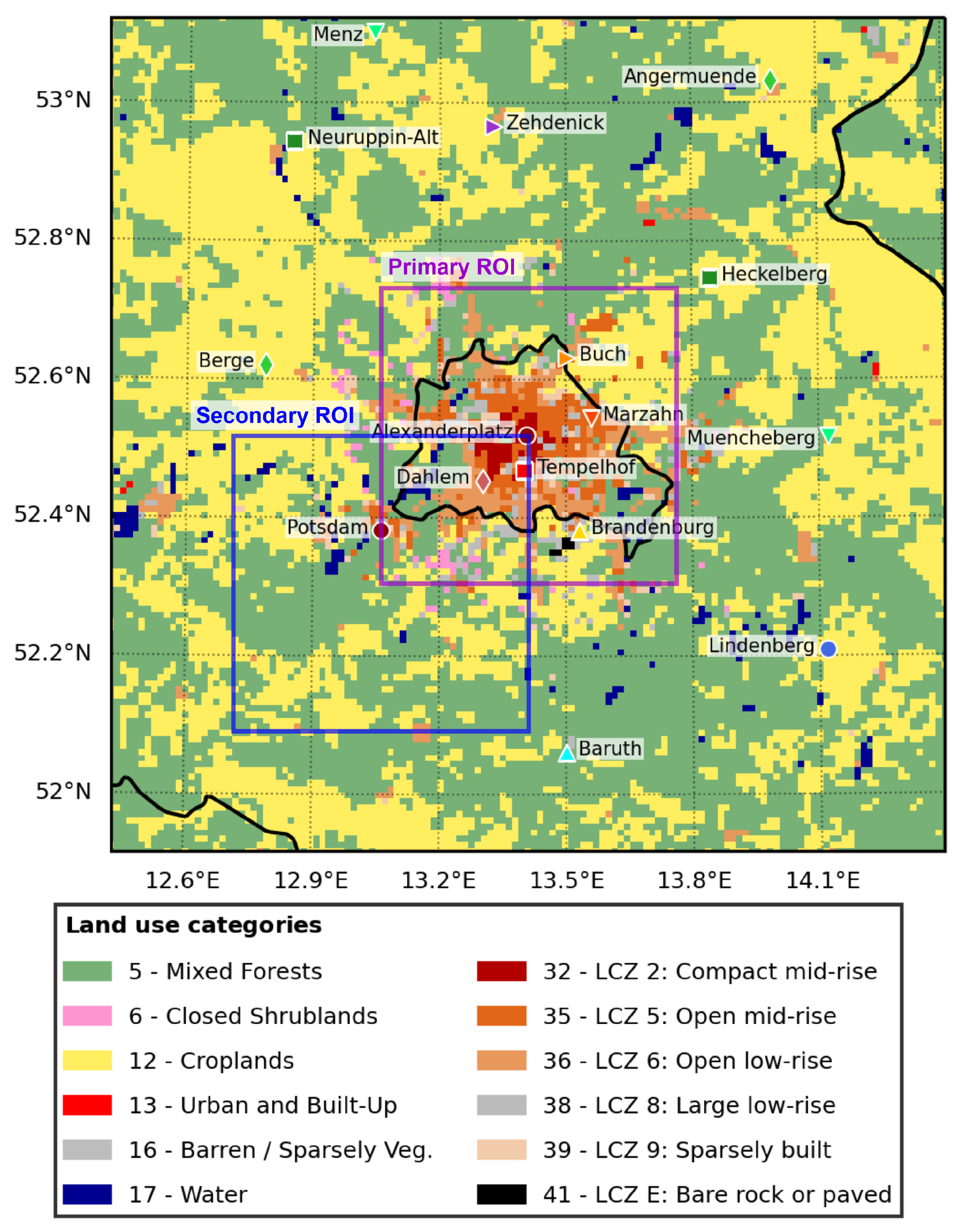
Figure 1. Land–use categories of the finest domain d03 of the WRF mesoscale model setup, where only occurring categories are shown. Also shown are positions and labels of DWD measurement stations used for model validation. The primary region of interest (ROI) was used for training the statistical downscaling models and the secondary ROI was used for additional validation of the deep learning model on mostly unseen data.
Remotesensing 15 04447 g001
Figure 2. Data splitting into training, validation, and testing sets. The data were split into 18 equal parts, where each part was approximately one month in length. The splits into different testing periods are denoted by index j and the split into different training/validation periods is denoted by index i. There are a total of 63 different split sequences ( J = 9 testing splits and I = 7 training/validation splits for each testing split).
Remotesensing 15 04447 g002
Figure 3. Deep learning downscaling model: U-Net variant “3D-space-time-residual”.
Remotesensing 15 04447 g003
Figure 4. Time-averaged model biases (98th percentile) for both the linear regression and the deep learning model.
Remotesensing 15 04447 g004
Figure 5. Time-averaged model inputs, outputs, and predictions for the deep learning model for different seasons.
Remotesensing 15 04447 g005
Figure 6. Box plots indicating the spatial variation of the error metrics within the 48 × 48 pixels of the core domain averaged for different seasons—full year, winter, spring, summer, and fall.
Remotesensing 15 04447 g006
Figure 7. Spatially-averaged time-series results for the deep learning model for different seasons. On the left-hand side, the daily average temperatures are shown for each day of the season, and on the right-hand side, the averaged temperature profile is shown for each hour of the day.
Remotesensing 15 04447 g007
Table 1. Discretization parameters to define the WRF domains d01, d02, and d03.
WRF Parameterd01d02d03
Lateral grid spacing9 km3 km1 km
Starting index in parent grid13637
Number of lateral grid points110118136
Vertical first full layer thickness10 m10 m10 m
Number of vertical grid points616161
Table 2. Metrics for both models evaluated over the last 12 months of the full 18-month period (avoiding repeating seasons).
MetricMLR ModelDL Model
MBE0.195  ° C0.350  ° C
MBE98P (98th percentile)−1.47  ° C−0.430  ° C
MAE1.49  ° C1.36  ° C
MAE98P (98th percentile)1.99  ° C1.80  ° C
RMSE1.91  ° C1.77  ° C
RMSE98P (98th percentile)2.50  ° C2.24  ° C
R 2 0.9440.952
PSNR28.429.0
SSIM0.9690.977
P( AE < ° C)0.7210.770
Table 3. Metrics calculated for the four different seasons from the predictions of the deep learning model (for each metric, the best-performing seasonal value is in bold font).
MetricWinterSpringSummerFall
MBE ( ° C)−0.0040.8860.3490.159
MAE ( ° C)1.381.51.251.34
RMSE ( ° C)1.781.921.681.68
R 2 0.7910.9050.8900.941
PSNR2928.329.429.5
SSIM0.9820.9740.9780.976
P( AE < ° C)0.7590.7280.8190.774
Table 4. Metrics evaluated over the last 12 months of the full 18-month period for the primary and the four secondary regions of interest.
MetricPrimary ROISW ROISE ROINW ROINE ROI
MBE ( ° C)0.3500.6070.6250.4540.471
MBE98P ( ° C)−0.430−0.575−0.604−0.881−0.825
MAE ( ° C)1.361.541.531.461.47
MAE98P ( ° C)1.801.681.831.751.86
RMSE ( ° C)1.771.981.961.881.89
RMSE98P ( ° C)2.242.122.312.212.39
R 2 0.9520.9400.9430.9470.947
PSNR29.028.028.128.528.4
SSIM0.9770.9770.9770.9740.974
P( AE < ° C)0.7700.7110.7180.7390.739
Disclaimer/Publisher’s Note: The statements, opinions and data contained in all publications are solely those of the individual author(s) and contributor(s) and not of MDPI and/or the editor(s). MDPI and/or the editor(s) disclaim responsibility for any injury to people or property resulting from any ideas, methods, instructions or products referred to in the content.