Mapping Buildings across Heterogeneous Landscapes: Machine Learning and Deep Learning Applied to Multi-Modal Remote Sensing Data

Abstract

We describe the production of maps of buildings on Hawai’i Island, based on complementary information contained in two different types of remote sensing data. The maps cover 3200 km² over a highly varied set of landscape types and building densities. A convolutional neural network was first trained to identify building candidates in LiDAR data. To better differentiate between true buildings and false positives, the CNN-based building probability map was then used, together with 400–2400 nm imaging spectroscopy, as input to a gradient boosting model. Simple vector operations were then employed to further refine the final maps. This stepwise approach resulted in detection of 84%, 100%, and 97% of manually labeled buildings, at the 0.25, 0.5, and 0.75 percentiles of true building size, respectively, with very few false positives. The median absolute error in modeled building areas was 15%. This novel integration of deep learning, machine learning, and multi-modal remote sensing data was thus effective in detecting buildings over large scales and diverse landscapes, with potential applications in urban planning, resource management, and disaster response. The adaptable method presented here expands the range of techniques available for object detection in multi-modal remote sensing data and can be tailored to various kinds of input data, landscape types, and mapping goals.

1. Introduction

Automated mapping of the built environment using remote sensing data is a rapidly growing field. This growth is driven by recent advances in machine learning, the increasing availability of high-quality data, and shifts in patterns of human habitation [1]. In particular, approaches that take advantage of recently developed machine learning techniques and multiple data modalities (e.g., Light Detection And Ranging [LiDAR], synthetic aperture radar [SAR], high-resolution imaging, imaging spectroscopy) are currently the focus of intensive research [2]. In this paper we develop, describe, test, and apply a method that takes advantage of the complementary information contained in LiDAR and spectroscopic data. The method combines a convolutional neural network and gradient boosting trees to locate residential buildings in a wide variety of landscape types. We use this method to produce maps of buildings over 3200 km² of Hawai’i Island, and we demonstrate that it yields high-quality results.

As an island with three active volcanoes, an accurate inventory of Hawai’i Island’s built environment is essential for emergency planning and disaster response [3]. In addition, much development on the island has taken the form of scattered, rural construction. Since this ‘rural residential development’ (RRD) can affect wildlife habitat, biotic interactions, and ecological processes [4], it is important to establish methodologies for mapping and monitoring RRD in Hawai’i and elsewhere. Moreover, many of the ~70,000 households on the island have on-site wastewater disposal systems (OSDS; cesspools or septic tanks) that pose a threat to groundwater and the marine environment [5,6]. Maps of houses and, by extension, their OSDS are needed to enable, for example, spatially explicit, hydrogeological modeling of wastewater transport to nearshore waters. Here, we focus on mapping residential buildings in three large regions of Hawai’i Island that are a particular focus of efforts to develop data-driven tools to support ridge-to-reef stewardship for the island.

The literature on remote sensing-based building detection and urban land cover classification contains much methodology that may be relevant to mapping Hawai’i Island’s buildings. That body of work can be categorized in terms of several characteristics: input data, setting (e.g., urban, rural), spatial scale, final product (pixel-wise classification vs. database of discrete objects), and analysis approach (traditional/feature engineering vs. deep learning). In feature engineering, a human carries out the process of selecting, manipulating and transforming raw data into features that can be used for machine learning. Random forests, support vector machines (SVMs), and gradient boosting with decision trees are common feature engineering applications. Deep learning, a subset of machine learning, omits the feature engineering step and instead uses nonlinear processing to extract features from data and transform the data into different levels of abstraction. Convolutional neural networks (CNNs) are an example of a deep learning method.

Regarding input data, high-resolution (<1 m) remotely sensed RGB images are widely available, and various kinds of RGB image have been used extensively in the development of deep learning models for computer vision tasks. High-resolution imaging and deep neural networks have thus been used to produce the largest-scale databases of building footprints, which are now available for the African continent [1], the United States [7,8], and indeed over much of the world [9]. The dataset produced by [8] includes footprints for 65,224 buildings on Hawai’i Island. However, that database is based on satellite imagery of unspecified vintage (mean year = 2012), and omits numerous buildings constructed since its release.

To produce updated maps for Hawai’i Island, we opted to use high-resolution (1–2 m) airborne LiDAR and imaging spectroscopy data collected over a large fraction of the island since 2016. In general, combining multiple types of data allows for the incorporation of different kinds of information. Here, LiDAR reveals the 3D structure of objects in the landscape, while imaging spectroscopy gives information about their 2D shape and material composition [10]. Rather than attempting to maximize detection rates and minimize contamination using either data type alone, it should be possible to use each one to compensate for any weaknesses of the other.

However, three key knowledge gaps needed to be addressed in order to use these data modalities for detecting buildings in the context of this study. First, the 3200 km² area of interest covers a wide variety of environments. These environments are highly heterogeneous, differing in terms of building density, land cover (from dense vegetation to bare rock), and other characteristics. In contrast, LiDAR and imaging spectroscopy datasets have mainly been used to detect objects or produce pixel-based land cover maps for relatively small, urban areas (<few km²). Second, deep learning-based methods for image segmentation and object detection that have proven effective in other contexts have only been applied to LiDAR and imaging spectroscopy data, separately, within the last decade [11,12]. Third, analyzing data from a combination of remote sensing modalities using deep learning techniques is now an active area of research [2]. We now briefly review some of the literature that is relevant to analyzing LiDAR and imaging spectroscopy data, and multi-modal data using deep learning approaches. Then, we devise a method that is effective over large, heterogeneous areas.

Zhou and Gong [12] claimed to be the first to have combined LiDAR with deep learning for automated building detection. The paper addressed the identification of buildings before and after disasters. The authors ran digital surface models (DSMs) through a CNN trained using 10,000 manually labeled samples from NOAA’s Digital Coast dataset. They found that their method performed well compared to standard LiDAR building detection tools, especially for the post-hurricane data. Maltezos et al. [13] found that performance improved when they added “additional information coming from physics” to DSMs, such as “height variation” and “distribution of normal vectors”. Gamal et al. [14] directly analyzed the 3D LiDAR point cloud to avoid the loss of information involved in converting to a DSM.

Yuan et al. [15] reviewed the literature on segmenting remote sensing imagery using deep learning methods, including applications to “non-conventional” data such as hyperspectral imaging. They pointed out that, compared to other computer vision applications, semantic segmentation of remote sensing data is distinguished by a need for pixel-level classification accuracy (in particular, accurate pixel classes around object boundaries) and a lack of labeled training data. Recent advances in analyzing hyperspectral imaging were discussed. These included using a 1D CNN to extract spectral features and a 2D CNN to extract spatial features then using the combined feature set for classification, and analyzing a 3D data cube with a CNN that performs 3D convolutions.

Different remote sensing modalities can be combined and analyzed in a number of ways, tailored to the available data and their characteristics. Recent reviews have highlighted three approaches: fusion of the data into a single data cube, separate extraction of features from each dataset followed by fusion, or combining decisions obtained from each dataset alone [16]. As data types such as LiDAR and imaging spectroscopy possess distinct characteristics, much work has focused on feature extraction and fusion across different data types [2,16] (although see [17] for an example of data-level fusion). Early work applied established algorithms to identify and fuse features, followed by classification using a CNN [18]. More recent studies have identified neural network architectures that can improve feature extraction, selection, fusion, and classification [19,20,21].

In addition to these ‘parallel’ methods, sequential approaches can be employed to integrate the complementary information present in different types of remote sensing data. Sequential approaches have been applied to single remote sensing data types, such as passing features identified by a CNN to an SVM for classification [22]). They have also been used in conjunction with multimodal datasets, outside the context of deep learning [23]. However, to the best of our knowledge, deep learning-based, sequential approaches to integrating LiDAR and imaging spectroscopy data have not yet been explored.

In this paper we investigate such an approach. First, we applied a U-NET-based CNN to LiDAR data to perform a preliminary segmentation. We then improved the initial pixel classifications using a gradient boosting model whose predictor variables included both the initial CNN-based map and the imaging spectroscopy data. Finally, we applied a set of vector operations to further refine the final maps. The method is described in detail in Section 2. In Section 3 we illustrate the rationale for this choice of sequence, and we show how and why the mapping evolves at each step. We also discuss the quality of the final maps and how they relate to comparable products that have been published. We close by discussing the broader applicability of this method and the maps it has produced.

This is one of just a few publications to date that explores how deep-learning-based techniques can be applied to LiDAR and spectroscopic data for the purpose of detecting buildings over large, diverse regions. The paper also shows that gradient boosting with decision trees can be useful even in situations involving great spectral heterogeneity. Furthermore, it determines the ways in which different spectral regions help to refine the initial CNN-based classification. The method described here has been implemented using freely-available software. Given the large amount of high-quality data becoming available, and its many potential applications, we hope this paper adds a useful and accessible option to the remote sensing toolbox.

2. Materials and Methods

This study used LiDAR and imaging spectroscopy data from the Global Airborne Observatory (GAO [24]), obtained between 2016 and 2020. The GAO captured the LiDAR and spectroscopy data simultaneously, allowing tight alignment between the two instruments [24]. The imaging spectrometer aboard the GAO measures reflected solar radiance in 428 bands between 380 nm and 2510 nm with 5 nm spectral sampling. At the 2000 m nominal flight altitude of the Hawai’i campaign, the imaging spectroscopy pixel size is 2 m.

The LiDAR point clouds were processed into a raster DSM by interpolating the regional maximum elevation of all returns from all pulses using the “translate” filter and “gdal” writer contained in the Point Data Abstraction Library software package version 2.0.1 [25]. Window size was set to 1.0, with radius 0.71 and the “max” interpolation algorithm was used. This resulted in DSMs with 1 m resolution depicting the elevation of vegetation and building upper surfaces. Hillshade and canopy height images at 1 m resolution were derived using standard procedures. Eigenvector images were derived from the DSMs by fitting a plane through the surface data within a 9 m × 9 m window around each pixel. The x, y, and z components of the normal vector to this plane, as well as the surface variation around this plane, were stored in a new four-band map.

The radiance data were transformed by first band-averaging into 214 bands of 10 nm spacing to reduce the noise within each spectrum. These maps were then processed with atmospheric correction software (ACORN v6; AIG, Boulder, CO, USA) to retrieve reflectance spectra. Reflectance maps were orthorectified using a calibrated camera model and a ray-tracing technique with the LiDAR-derived surface elevation maps [24]. A brightness-normalized version of the reflectance data cubes was made by dividing the spectrum at each pixel by the total reflectance in the spectrum (i.e., dividing by its vector norm), and both the original and brightness-normalized data cubes were incorporated into further analyses.

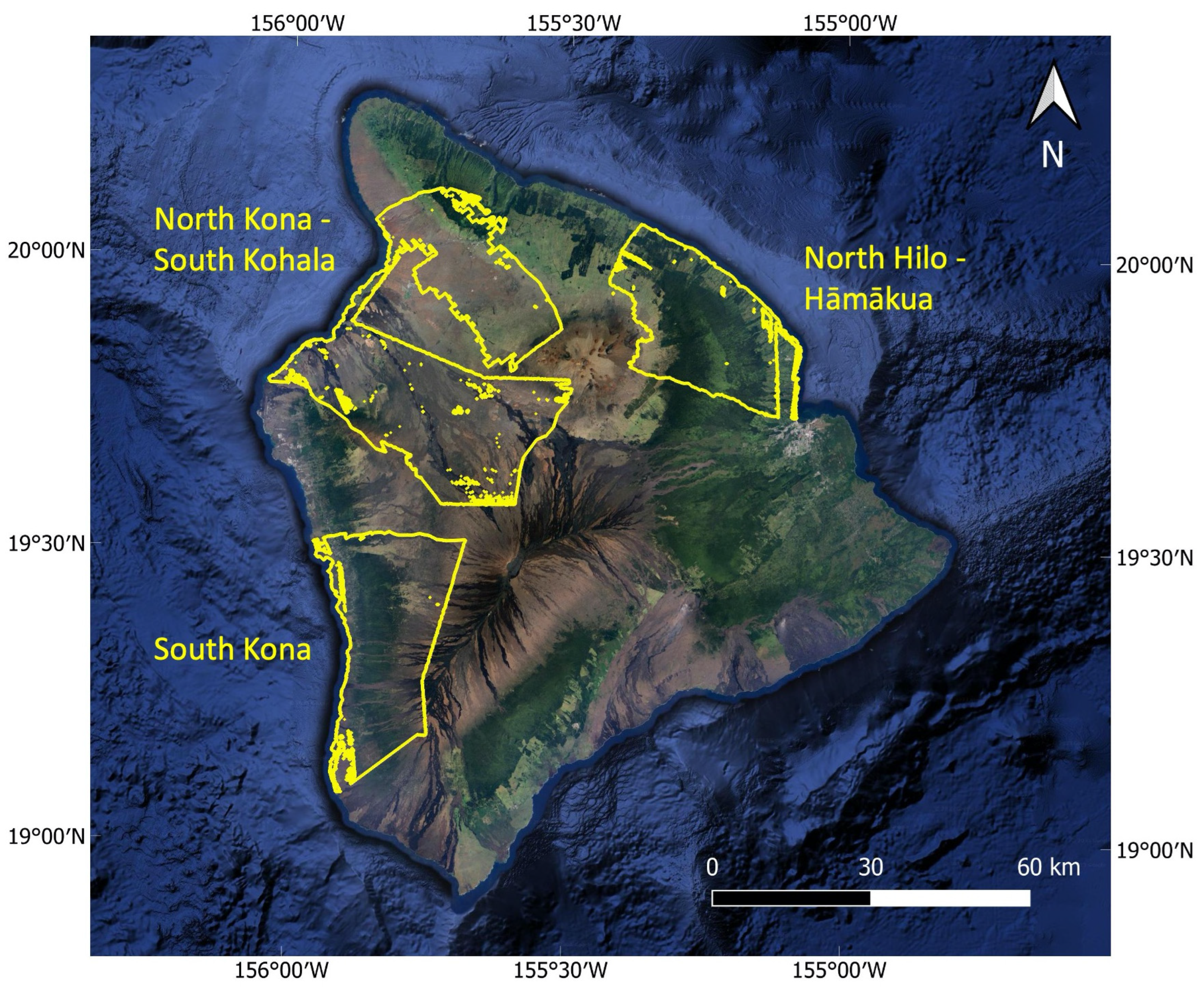
The three areas mapped for this work (Figure 1) were selected as part of a larger effort to provide data-driven decision support on Hawai’i Island. They are highly heterogeneous, covering a wide range of characteristics. In North Hilo—Hāmākua, high annual rainfall supports small-scale agriculture, timber plantations, and native and non-native forests. This area hosts a number of small villages as well as low-density rural development. In North Kona—South Kohala, the island’s main resort areas and some coastal development sit against a backdrop of dry, fire-prone, non-native grasslands and shrublands. Nearshore ecosystems in this area have suffered from high sediment and nutrient loads from coastal erosion, OSDS and other sources [6,26,27]. The South Kona district is host to rural residential and agricultural development in a diversity of environments (such as bare lava flows, forest, orchards, and pastureland), as well as scattered coastal developments and relatively undisturbed coral reefs. With the exception of the Waikoloa Village area in North Kona—South Kohala, and small sections of South Kona and North Hilo—Hāmākua, the parts of the study geographies that lack GAO data coverage are essentially uninhabited.

To generate infrastructural maps of the three study areas, we first employed a CNN to assign probabilities that pixels in LiDAR-derived data belonged to ‘building’ or ‘not-building’ classes (Figure 2). Briefly, a CNN consists of layers of nodes that receive input from the previous layer, convolve the input with a filter (kernel), and pass the result to nodes in the subsequent layer that perform similar operations. The convolutions initially detect simple shapes (e.g., edges) in the input image, then the passage through subsequent layers gradually builds up more and more complex features. The connections between layers are assigned weights that are adjusted during an optimization process, giving higher weights to more informative features and converging on the set of features that leads to the most accurate classification of a labeled training data set.

Labeled training/validation and test data for the CNN were generated by manually outlining rooftops in the DSMs. All visually identifiable buildings were labeled, regardless of perceived function, then those with area <50 m² were excluded. Locations for gathering training/validation data were initially chosen based on (1) the presence of buildings for the model to learn from, (2) the presence of fairly closely-spaced buildings, so the training set would not be dominated by non-building pixels, and (3) landscape characteristics across the range spanned by the three geographies of interest.

Preliminary experiments were carried out on training data from three locations and adjacent test regions. Based on the results obtained, data were gathered from an additional six training and five test locations. The full training dataset contains 2083 building outlines and covers 34 km². The full test dataset contains 1124 building outlines and covers 16 km². This conservative ~65:35 train:test split was chosen in order to give confidence that the model was performing adequately over a wide range of landscape types, in visual as well as statistical checks. The test regions were only used for the purpose of evaluating model quality at each step, after training had been completed.

The freely-available Big Friendly Geospatial Networks (BFGN) package [28] was used to process model training data, train a CNN to assign “building” and “not-building” probabilities to LiDAR pixels, and apply the trained model to the test datasets. BFGN implements a version of the U-NET CNN architecture [29], adapted to handle different input sizes [30], to perform semantic segmentation of remote sensing images. The package is designed for transparent handling of geospatial data and has previously been used to map termite mounds in LiDAR data [30].

In the default configuration used for this project, the CNN consists of 32 layers and 7994 trainable parameters. Of the 32 layers, 24 are convolutional layers, and the remainder perform batch normalization, max pooling, up-sampling, and concatenation. Batch size = 32 was used together with batch normalization, and the “building” class was given higher weight during model training, due to its small size relative to the “not-building” class. The files recording the package/model configuration can be found as described in the Data Availability Statement. The training and application of all models discussed in this paper were carried out on a GTX1080 GPU and took a few minutes to a few hours, largely depending on the spatial coverage and number of bands of the data.

The model was trained on the combined data for all training regions. During pre-processing with BFGN the training data are split into small, square ‘windows’, and three different window sizes were tested (see the supplementary material for [31] for further explanation). Training was also performed separately on the DSM, hillshade, and eigenvector data, resulting in a total of nine trained models. The models were applied to the training and held-out test regions, producing nine per-pixel building probability maps per region (Figure 2). Ensemble maps were created by averaging the nine maps for each region. This had the effect of reducing the number of false positives, which were only weakly correlated between different combinations of input data type and window size, while preserving true positives. The ensemble maps were then interpolated to the same 2 m pixel size as the imaging spectroscopy.

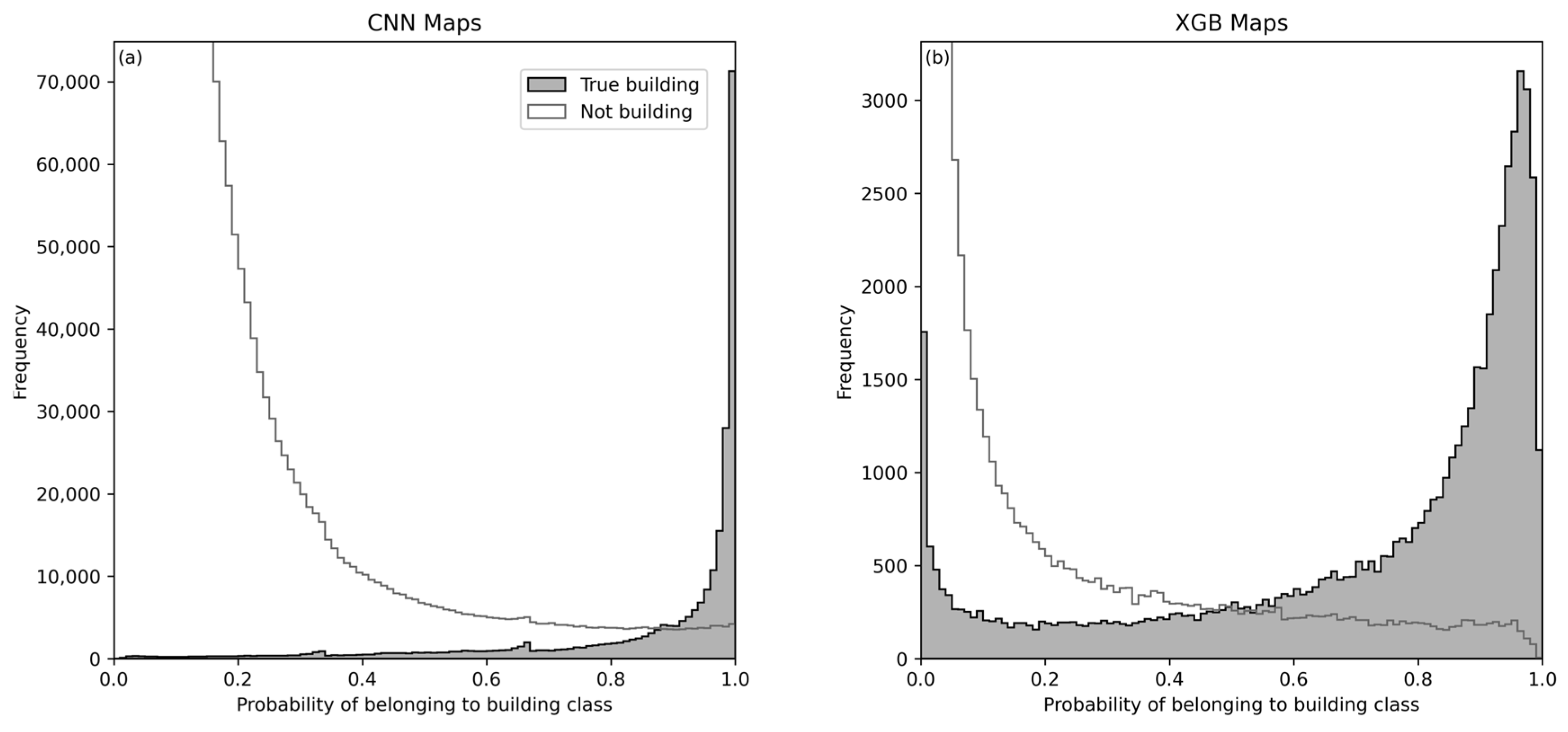
The ensemble CNN-based maps, imaging spectroscopy data cubes, and canopy height images for the training regions were used as input to the XGBoost model v 1.6.2 [32] to reclassify the pixels (Figure 2). XGBoost is an implementation of gradient boosting with decision trees, in which successive trees are trained iteratively with each new tree trying to correct the errors of the previous one. This results in a final model that can accurately predict the target variable even when the relationships between variables are complex. Among gradient boosting implementations, XGBoost is known for its efficiency, flexibility, and ability to handle missing data, as well as a large and active user community [33].

Gradient boosting trees are capable of handling high-dimensional datasets, and we were also interested in finding out which spectral regions would be particularly informative. Therefore all 147 imaging spectroscopy bands not compromised by strong atmospheric H₂O absorption were included in the model training set. As with the CNN, a set of slightly different map versions were created, using slightly different subsets of the training data and spectra that had and had not been brightness-normalized, and averaged into an ensemble map. At this point, pixels with building probability ≥ 0.2 were classified as buildings, and others as not-building.

The maps were converted to vector space, further refined by applying a set of simple vector operations, then converted back to raster format (Figure 2). The vector operations consisted of (1) applying a −1 m buffer to each polygon, (2) rejecting polygons < 25 m², (3) rejecting polygons that coincided with roads and the coastline of the island, (4) closing holes, and (5) representing each polygon by its minimum oriented bounding box. The CNN-based and gradient boosting models derived from the training region data and these final cleaning operations were then applied to the entirety of the three study geographies. Ipython notebooks showing the full process are available as described in the Data Availability Statement.

3. Results

Here, we first describe the steps in the modeling process, showing how and why each one addresses deficiencies in the previous step (Section 3.1). We then assess the quality of the maps using a set of complementary measures (Section 3.2). As imaging spectroscopy is an important and novel component of the analysis, we also discuss the spectral regions that turned out to be informative in segmenting the data (Section 3.3).

3.1. Overview of the Mapping Process

Figure 3 illustrates steps in the map-making process for a variety of locations within the test regions. In the first step, the CNN assigned high building probability to the majority of building pixels. However, the CNN also incorrectly assigned high building probabilities to many non-building pixels. Many of the false detections were tree crowns that structurally resemble buildings (Figure 3, bottom row), while ground features on lava flows (Figure 3, penultimate row) and along streams, coastline, road edges, etc., accounted for many others. Figure 4a shows that these features could not be excluded using a simple probability threshold. Rejecting pixels that had been classified as buildings with, say <90% probability would exclude many true building pixels, while lower thresholds would fail to remove a large number of false positives.

Instead, we incorporated information from spectroscopy to aid in identifying false positive pixels. To illustrate the kind of information available, Figure 5 shows spectra of a few common objects and materials in the building and not-building classes. Tree crowns, which comprise many of the false positives in the CNN map, have a highly distinctive spectrum characterized by the “red edge” around 700 nm, where absorption from chlorophyll molecules gives way to strong scattering in the near-infrared. Further into the infrared, the spectrum is shaped by broad H₂O absorption bands. Many buildings on Hawai’i Island have metal roofs, and their spectra are heavily influenced by the chemical makeup of the coatings that have been applied [34,35]. In Figure 5, the white-painted roof has high reflectance in the visible part of the spectrum, which gradually declines into the near-IR. The blue-painted roof, in contrast, contains a wide absorption trough from ~1100–1700 nm caused by cobalt ions in blue pigments [34]. Asphalt shingle roofs and lava rock have similar spectra, characterized by low and relatively constant reflectance throughout. All of these spectra have hydrocarbon absorption bands at approximately 1180 nm, 1450 nm, 1715 nm, 1940 nm, 2130 nm, and 2260 nm, which may be from petroleum-based products such as paint binders [34,36] or constituents of plants. Absorption bands from many other substances may also be present, such as iron oxides at 520 nm, 670 nm, and 870 nm in oxidizing metals [37].

The spectra therefore contained a large amount of potentially useful information. However, there was marked intra-class variation even in the limited selection of materials shown in Figure 5. The spectra varied in terms of absolute reflectance, overall spectral shape, and the presence and strength of individual absorption features. Moreover, there was considerable overlap between classes: asphalt shingle roofing and lava rock are more similar to each other than to other members of their own class. In initial testing, we did not find XGBoost to be effective in classifying pixels based on spectroscopy alone. However, including the CNN-based probabilities (and canopy height images) as predictor variables allowed XGBoost to produce maps that were much cleaner than those derived from the CNN alone (Figure 3, column d).

Figure 4b shows that the XGBoost model still did not provide a complete separation between building and not-building pixels in probability space. However, applying a further set of simple operations resulted in final maps with a high detection rate and few false positives. We first created binary maps in which all pixels with building probability > 0.2 were assigned to the ‘building’ class. This threshold approximately corresponds to an inflection point in probability space below which the likelihood of false positives rises rapidly (Figure 4b).

In the binary maps, the remaining false positive pixels tended to occur in very small groups (they were often the edges of tree crowns and ground features that were incompletely removed by the XGBoost model), around the edges of true buildings, or coincident with roads or coastline (Figure 3, column d). They were thus amenable to removal by the set of simple vector operations described in Section 2. Applying small negative buffers improved the separation of closely-spaced buildings and removed artefacts around building edges. Excluding polygons with area < 25 m² removed residual false positive pixels that clustered in small groups. Polygons that intersected with roads and the coastline of the island were also likely to be false positives and were rejected. Closing holes in polygons and representing each polygon by its minimum oriented bounding box helped to fill in small gaps and improved the final representation of each building.

3.2. Quantitative Map Characteristics

To aid comparison with various metrics that may be presented by other authors, we assess the quality of the final maps in three ways. These are presented in increasing order of rigor. First,

Table 1. Polygon-based performance metrics for test region maps produced at two intermediate stages in the mapping process, and for the final maps (see Figure 2 and Figure 3).

Map	Precision	Recall	F1-Score
CNN-based	0.90	0.76	0.81
XGBoost-based	0.80	0.92	0.85
Final	0.99	0.85	0.92

gives the polygon-based precision, recall, and f1-score for the intermediate (CNN-based and XGBoost-based) and final maps. These numbers were calculated based on the number of modeled buildings that are intersected by a labeled building, and vice versa. Polygon-based recall essentially asks, ‘what fraction of known buildings are overlapped by a modeled building?’. Similarly, polygon-based precision measures the fraction of modeled buildings that have corresponding, known buildings. These are whole-object metrics that are not sensitive to misclassifications at the pixel level.

Overall, the maps achieve high values of recall, precision, and f1-score. However, Figure 6a shows that polygon-based recall depends on building area. At the 25th, 50th, and 75th percentiles of labeled building areas (133 m², 218 m², and 289 m²), recall = 0.84, 1.0, and 0.97, respectively. At areas < 90 m², which make up 14% of the labeled buildings, recall ≤ 0.70.

Beyond the simple detection of structures in the correct locations, the accuracy of the modeled building sizes is also important. In a scatter plot of labeled and modeled building sizes, most buildings clustered around the 1:1 line (Figure 6b). The median absolute error in area over all test region buildings was 15%. Most of the buildings above the 1:1 line had neighbors within 6 m (3 imaging spectroscopy pixels). These closely-spaced buildings were often incorrectly identified as single, larger structures. Another set of outliers consisted of buildings with large true sizes but small modeled sizes. These were usually commercial or agricultural structures, including irregular clusters of small sheds, that were infrequent in the training data set. Other points that lie below the 1:1 line were often seen to be buildings with complex roof structures that were not clearly recognized as buildings by the CNN and/or roofs that were partially occluded by vegetation.

A third pair of metrics, pixel-based precision and recall, reflect the number of individual pixels that were correctly classified. High recall and precision values indicate that not only were structures detected in the correct locations and with accurate sizes, but that their morphology also closely matched that of each labeled building. In our maps, pixel-based recall was 0.71 and precision was 0.78. These numbers include all pixels, and therefore all building sizes, in the test regions.

3.3. Influential Spectral Regions

Modeling entire spectra, without first applying dimensionality-reduction techniques, permits some insight into the spectral regions that are important in classifying pixels. Figure 5 shows the most influential wavelength intervals when using original and brightness normalized spectra. On the one hand, the absolute reflectance of an individual pixel may be related to factors such as viewing angle which are not related to the composition of the materials represented in that pixel, which argues for brightness-normalizing the data. On the other hand, visual examination of the data cubes showed that buildings tended to stand out in absolute reflectance against other components of the landscape, especially at short wavelengths. It seemed reasonable to model both variations, and indeed the model performance statistics were almost identical in each case.

We quantified feature influence using SHapley Additive exPlanations (SHAP values [38]). SHAP values estimate the contribution of each feature to a model’s output by evaluating how much the presence or absence of the feature changes the predicted output when compared to a baseline prediction (usually the average value of the target variable for the entire training dataset). The resulting values indicate the relative importance of each feature and how much each feature contributes to the model’s predictions, accounting for interactions between features. Here, high positive SHAP values mean that a wavelength interval was influential in placing a given pixel into the ‘building’ class.

CNN model probability (not shown in Figure 5) was always the most influential variable, and the canopy height map was also always in the top three. Among the influential spectral bands, many occur at the short-wavelength end of the spectrum, especially for the not-normalized data. This was consistent with the generally higher short-wavelength reflectance of the rooftop spectra in Figure 5 (although this is not a comprehensive sample).

Some other influential regions may be associated with the particular chemical make-up of materials and objects in the landscape. For example, the region around 700 nm, where vegetation reflectance changes rapidly due to absorption by chlorophyll, is one of the more informative. Influential features in the vicinity of 1100–1200 nm likely reflect differences in H₂O absorption across many different materials. At the longest wavelengths, high SHAP values appear to be associated with hydrocarbon absorption features.

While some wavelength regions are more informative than others, there are no discrete absorption features that greatly outweigh others in importance; influence is distributed fairly evenly over the spectrum. This is not surprising, given the high intra-class spectral variation and the resemblance between materials like shingle roofing and lava rock substrate. Rather, XGBoost is able to model very complex relationships between spectra and building/not-building classification when used in conjunction with supporting information like the CNN-derived building probabilities for each pixel.

4. Discussion

We found the combination of a CNN and gradient boosting with decision trees to be an effective means of segmenting LiDAR and imaging spectroscopy data into building and not-building classes in a highly heterogeneous landscape. The CNN was effective at detecting buildings in the higher-resolution LiDAR data, but also misclassified objects such as tree crowns and ground surface features. Including the CNN-derived probability map along with the imaging spectroscopy bands as features in a gradient boosting model reduced the number of false positive detections. This was in spite of high intra-class variation in spectral properties that results from the wide variety of roofing materials and coatings in the study areas, and spectral similarity between some roofing materials (e.g., asphalt shingle) and landscape features (e.g., rocks). A subsequent set of simple vector operations further refined the final maps.

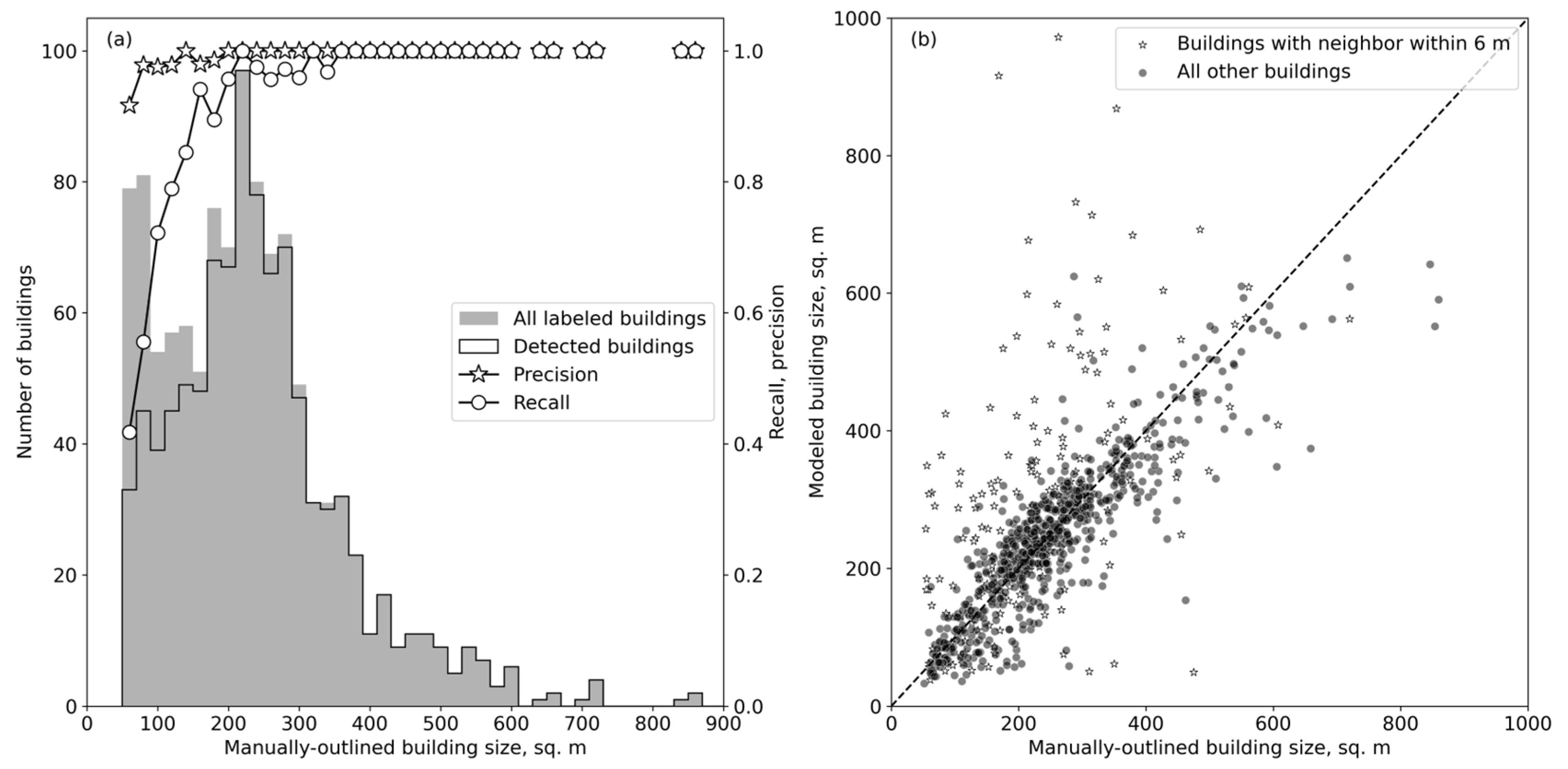
At the median building size in the test dataset, building detection rates approached 100%. Detection rates were lower for small buildings, which may be for several reasons. First, smaller structures were difficult for the CNN to detect against the background in the 1 m LiDAR pixels, meaning that the CNN-derived probability maps frequently assigned low or zero probability to pixels within small buildings. Then, the 2 m spectroscopy pixels may have been significantly ‘contaminated’ by non-building material, which would likely make them more difficult to classify. We also speculate that small buildings are more likely to be agricultural structures (e.g., polytunnels) and informal buildings (sheds, canopies), and this category may therefore include spectra that are both more diverse and less well-represented in the training dataset.

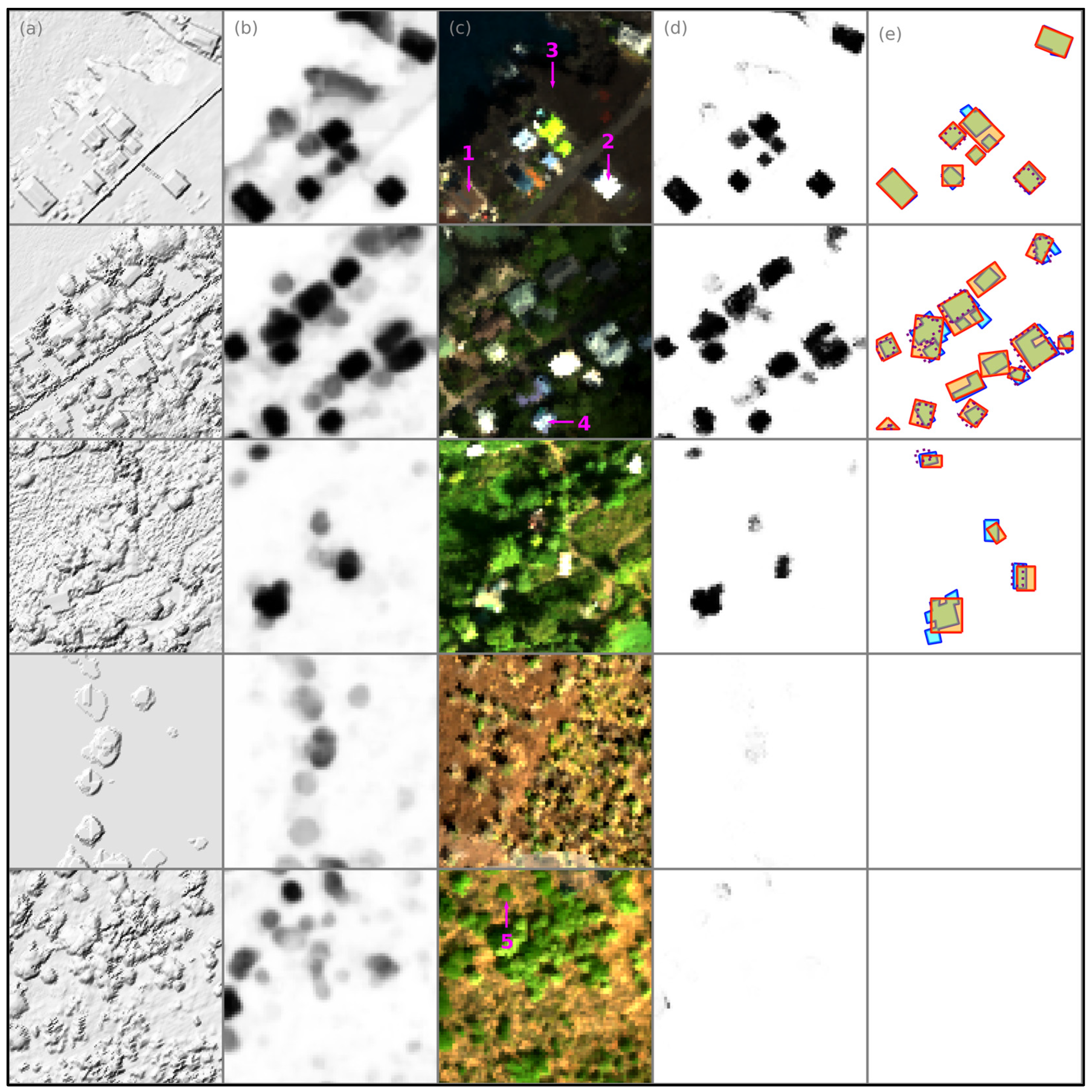
Other LiDAR- and imaging spectroscopy-based building detection methods tend to cover landscapes that are much smaller and/or more homogeneous than the three Hawai’i Island geographies mapped in this study. The most relevant comparison is the USBFD [8], which is based on satellite imagery and contains footprints for 11,283 buildings in these three areas. Visually, the maps that we present appear similar in quality to the USBFD (Figure 3, column e), with three main differences. First, the USBFD polygonization algorithm more closely approximates building outlines than we attempted to, meaning that non-rectangular structures are more accurately delineated in the USBFD. Second, in many locations there are offsets between buildings in the USBFD and both our LiDAR and spectroscopy data and Google satellite images. This is presumably related to the registration of the satellite images in which the USBFD footprints were detected. Third, numerous buildings appear on our maps but not in the USBFD. This is likely mainly because many buildings have been constructed since the acquisition of the data used for the USBFD for Hawai’i. However, there are also locations (such as the village of Papa’aloa in the Hāmākua district) where the USBFD contains only a small fraction of buildings present, despite all houses dating from the 20th century.

The USBFD reports pixel-based precision = 0.94 and recall = 0.96 for their test datasets. This is much higher than the values that we obtain (precision = 0.78 and recall = 0.71, over all building sizes; Section 3.3). However, ref. [39] show that actual recall values in the USBFD are a strong function of building size. Although recall ranges from 0.93–0.99 in buildings > 200 m², ref. [39] find that it falls to 0.37–0.73 when calculated over all building sizes in their test datasets. This relationship between recall and building area is consistent with our findings in Figure 6a and highlights the difficulty in making straightforward comparisons between published results.

Convolutional neural networks (CNNs) and other machine learning algorithms are rapidly gaining popularity for remote sensing-based computer vision tasks in fields such as ecology, conservation, and planning [31,40]. The development of accessible tools, including the BFGN package utilized in this study [28], is making these advanced techniques more widely available to non-specialists. The combination of CNNs with other machine learning algorithms, as demonstrated in this paper, expands the range of techniques available for using complementary information in multi-modal data, and allows the user to be flexible and adapt to a variety of different data types.

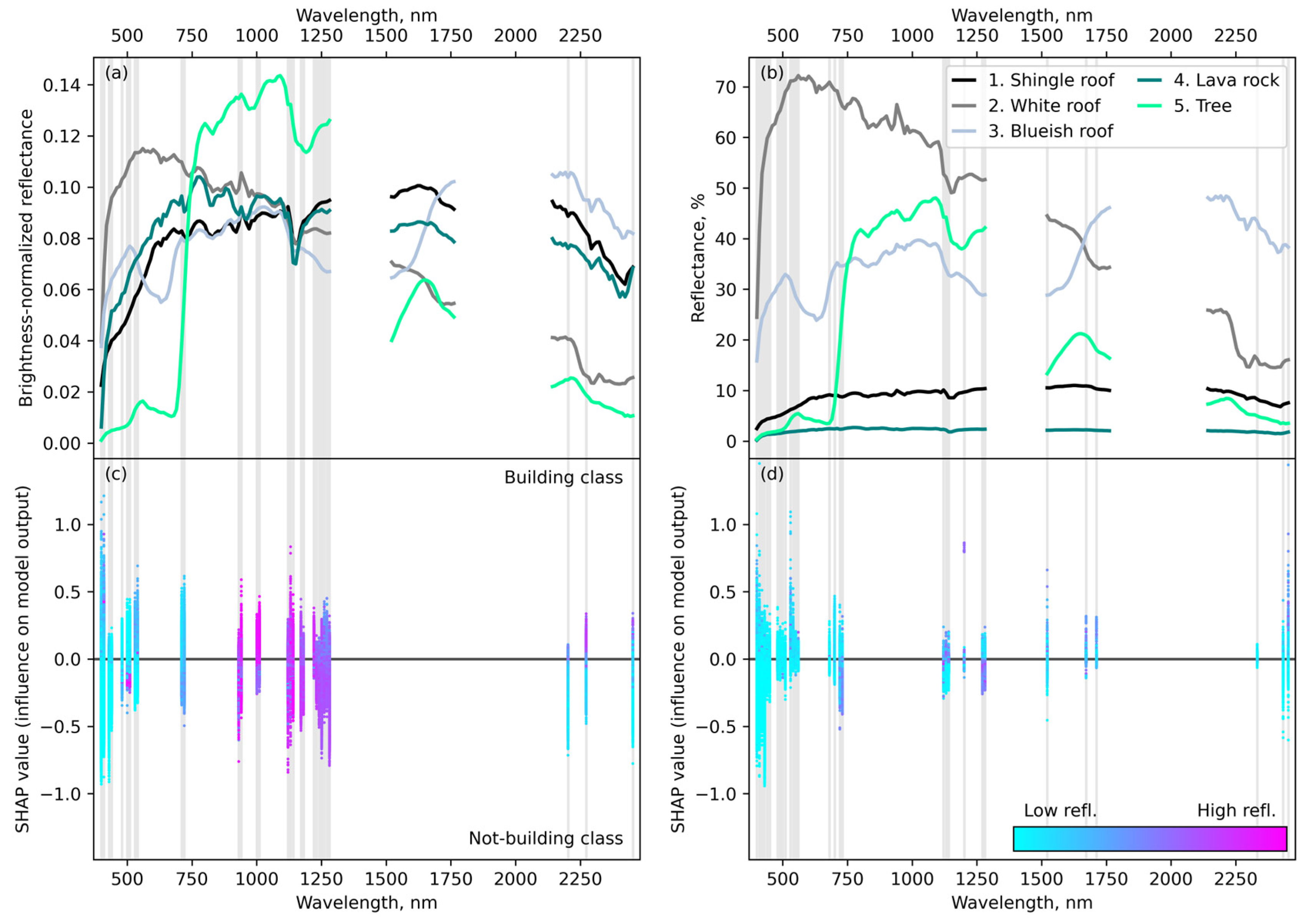
Gradient boosting algorithms have received much attention in recent years, but few applications to spectroscopic data have been described in the literature so far. In a recent study, ref. [41] used XGBoost to classify spectra of dwarf and giant stars. They concluded that, while the algorithm identified spectral features traditionally used by astronomers for stellar classification, it also identified new diagnostic regions that significantly contribute to the differentiation between classes. This conclusion was based on the number of times each wavelength band was used in the decision trees. Here, we show that gradient boosting trees are also useful in situations involving much greater spectral diversity. Extending beyond feature use counts, we used SHAP values to identify influential spectral regions. We found that although few wavelength bands disproportionately influenced the classification, short wavelengths (<500 nm) tended to be among the most important. Absorption features associated with chlorophyll, H₂O, and hydrocarbons were also influential.

The methodology presented in this study has potential for mapping other landscape components with well-defined spatial structure, such as orchard crops and roads, in rural and peri-urban areas. Furthermore, it can be customized to use other data sources that contain information about the structure and composition of landscape features, as well as to accommodate the specific conditions of different landscapes. For instance, in a more uniform landscape than the one examined in this research, multi-band or RGB imaging could serve as a satisfactory substitute for imaging spectroscopy. Similarly, if the goal is to detect small structures, it may be feasible to achieve this by carefully selecting representative training spectra based on knowledge of materials used locally. These possibilities highlight the versatility of multi-sensor data, and their potential for broadening the scope of remote sensing applications.

One issue faced during this work was the manual and time-consuming process of labelling the training data. Determining what constituted a building was not always straightforward; the difference between small houses, non-residential buildings, and structures such as temporary canopies, water tanks, piles of abandoned vehicles, etc. was not always clear. This complicated the assessment of model performance at the small end of the building size distribution. In addition, buildings separated by <3 imaging spectroscopy buildings tended to be incorrectly identified as single, larger structures. This mainly occurs in built-up areas that are connected to municipal sewer lines, rather than the rural residential development that is the focus of this work, so improving building separation was not considered a high priority. However, it may be possible to achieve better separation using traditional techniques such as watershed analysis, or by applying a CNN to the final maps.

The building maps produced using this methodology will be used within a decision support tool framework to assist hydrogeological modeling of residential wastewater transport. They will also be useful for many other purposes. For example, they may help to clarify OSDS numbers and locations on Hawai’i Island, which are currently uncertain [42]. Measures of building density may help local advocacy groups assess the viability of community-level micro-treatment plants, potentially a preferred alternative to OSDS [43]. The spectroscopic data available for the rooftops in this dataset could be used to assess indoor temperatures as the climate warms [44] or to help evaluate the potential environmental impact of contaminants in roofing runoff [45,46]. To allow for a broad range of uses, the maps are freely available as described in the Data Availability Statement.

5. Conclusions

We have shown that the combination of a CNN with gradient boosting decision trees can effectively identify buildings in LiDAR and imaging spectroscopy data, even in landscapes exhibiting high heterogeneity. In our maps of three diverse regions of Hawai’i Island, detection rates were high for typical residential buildings, while false positives were straightforwardly removed by simple vector-based operations. In common with existing building footprint datasets, detection rates were a function of building size, with small buildings more likely to be missed. This is likely due to their small size relative to the resolution of the remote sensing data and increased spectral heterogeneity among structures of this size.

Few studies had previously examined the use of gradient boosting trees for handling spectroscopic data sets. We found that they are useful even in situations involving a high degree of spectral diversity, and we identified spectral regions that appear particularly influential for classification. Based on the findings in this paper, these techniques may be adapted for mapping various landscape components or working with different data types, thereby broadening the scope of remote sensing applications. The flexibility to generate up-to-date building maps utilizing available data resources is a potent tool, aiding a wide array of applications from hydrogeological simulations to research into the ecological impacts of rural residential development.

References

1. Sirko, W.; Kashubin, S.; Ritter, M.; Annkah, A.; Bouchareb, Y.S.E.; Dauphin, Y.; Keysers, D.; Neumann, M.; Cisse, M.; Quinn, J. Continental-Scale Building Detection from High Resolution Satellite Imagery. arXiv 2021, arXiv:2107.12283. [Google Scholar] [CrossRef]
2. Li, J.; Hong, D.; Gao, L.; Yao, J.; Zheng, K.; Zhang, B.; Chanussot, J. Deep Learning in Multimodal Remote Sensing Data Fusion: A Comprehensive Review. Int. J. Appl. Earth Obs. Geoinf. 2022, 112, 102926. [Google Scholar] [CrossRef]
3. Laverdiere, M.; Yang, L.; Tuttle, M.; Vaughan, C. Rapid Structure Detection in Support of Disaster Response: A Case Study of the 2018 Kilauea Volcano Eruption. In Proceedings of the IGARSS 2020—2020 IEEE International Geoscience and Remote Sensing Symposium, Waikoloa, HI, USA, 26 September–2 October 2020; pp. 6826–6829. [Google Scholar]
4. Hansen, A.J.; Knight, R.L.; Marzluff, J.M.; Powell, S.; Brown, K.; Gude, P.H.; Jones, K. Effects of Exurban Development on Biodiversity: Patterns, Mechanisms, and Research Needs. Ecol. Appl. 2005, 15, 1893–1905. [Google Scholar] [CrossRef]
5. Wiegner, T.N.; Colbert, S.L.; Abaya, L.M.; Panelo, J.; Remple, K.; Nelson, C.E. Identifying Locations of Sewage Pollution within a Hawaiian Watershed for Coastal Water Quality Management Actions. J. Hydrol. Reg. Stud. 2021, 38, 100947. [Google Scholar] [CrossRef]
6. Yoshioka, R.M.; Kim, C.J.S.; Tracy, A.M.; Most, R.; Harvell, C.D. Linking Sewage Pollution and Water Quality to Spatial Patterns of Porites Lobata Growth Anomalies in Puako, Hawaii. Mar. Pollut. Bull. 2016, 104, 313–321. [Google Scholar] [CrossRef] [PubMed]
7. Yang, H.L.; Yuan, J.; Lunga, D.; Laverdiere, M.; Rose, A.; Bhaduri, B. Building Extraction at Scale Using Convolutional Neural Network: Mapping of the United States. IEEE J. Sel. Top. Appl. Earth Obs. Remote Sens. 2018, 11, 2600–2614. [Google Scholar] [CrossRef]
8. Microsoft USBuildingFootprints. Available online: https://github.com/microsoft/USBuildingFootprints (accessed on 16 December 2022).
9. Microsoft GlobalMLBuildingFootprints. Available online: https://github.com/microsoft/GlobalMLBuildingFootprints (accessed on 17 October 2022).
10. Kuras, A.; Brell, M.; Rizzi, J.; Burud, I. Hyperspectral and Lidar Data Applied to the Urban Land Cover Machine Learning and Neural-Network-Based Classification: A Review. Remote Sens. 2021, 13, 3393. [Google Scholar] [CrossRef]
11. Chen, Y.; Lin, Z.; Zhao, X.; Wang, G.; Gu, Y. Deep Learning-Based Classification of Hyperspectral Data. IEEE J. Sel. Top. Appl. Earth Obs. Remote Sens. 2014, 7, 2094–2107. [Google Scholar] [CrossRef]
12. Zhou, Z.; Gong, J. Automated Residential Building Detection from Airborne LiDAR Data with Deep Neural Networks. Adv. Eng. Inform. 2018, 36, 229–241. [Google Scholar] [CrossRef]
13. Maltezos, E.; Doulamis, A.; Doulamis, N.; Ioannidis, C. Building Extraction from LiDAR Data Applying Deep Convolutional Neural Networks. IEEE Geosci. Remote Sens. Lett. 2019, 16, 155–159. [Google Scholar] [CrossRef]
14. Gamal, A.; Wibisono, A.; Wicaksono, S.B.; Abyan, M.A.; Hamid, N.; Wisesa, H.A.; Jatmiko, W.; Ardhianto, R. Automatic LIDAR Building Segmentation Based on DGCNN and Euclidean Clustering. J. Big Data 2020, 7, 102. [Google Scholar] [CrossRef]
15. Yuan, X.; Shi, J.; Gu, L. A Review of Deep Learning Methods for Semantic Segmentation of Remote Sensing Imagery. Expert Syst. Appl. 2021, 169, 114417. [Google Scholar] [CrossRef]
16. Sun, X.; Tian, Y.; Lu, W.; Wang, P.; Niu, R.; Yu, H.; Fu, K. From Single- to Multi-Modal Remote Sensing Imagery Interpretation: A Survey and Taxonomy. Sci. China Inf. Sci. 2023, 66, 140301. [Google Scholar] [CrossRef]
17. Morchhale, S.; Pauca, V.P.; Plemmons, R.J.; Torgersen, T.C. Classification of Pixel-Level Fused Hyperspectral and Lidar Data Using Deep Convolutional Neural Networks. In Proceedings of the 2016 8th Workshop on Hyperspectral Image and Signal Processing: Evolution in Remote Sensing, Los Angeles, CA, USA, 21–24 August 2016. [Google Scholar] [CrossRef]
18. Ghamisi, P.; Plaza, J.; Chen, Y.; Li, J.; Plaza, A.J. Advanced Spectral Classifiers for Hyperspectral Images: A Review. IEEE Geosci. Remote Sens. Mag. 2017, 5, 8–32. [Google Scholar] [CrossRef]
19. Huang, J.; Zhang, X.; Xin, Q.; Sun, Y.; Zhang, P. Automatic Building Extraction from High-Resolution Aerial Images and LiDAR Data Using Gated Residual Refinement Network. ISPRS J. Photogramm. Remote Sens. 2019, 151, 91–105. [Google Scholar] [CrossRef]
20. Hosseinpour, H.; Samadzadegan, F.; Javan, F.D. CMGFNet: A Deep Cross-Modal Gated Fusion Network for Building Extraction from Very High-Resolution Remote Sensing Images. ISPRS J. Photogramm. Remote Sens. 2022, 184, 96–115. [Google Scholar] [CrossRef]
21. Feng, Q.; Zhu, D.; Yang, J.; Li, B. Multisource Hyperspectral and LiDAR Data Fusion for Urban Land-Use Mapping Based on a Modified Two-Branch Convolutional Neural Network. ISPRS Int. J. Geo-Inf. 2019, 8, 28. [Google Scholar] [CrossRef]
22. Xia, B.; Kong, F.; Zhou, J.; Wu, X.; Xie, Q. Land Resource Use Classification Using Deep Learning in Ecological Remote Sensing Images. Comput. Intell. Neurosci. 2022, 2022, 7179477. [Google Scholar] [CrossRef]
23. Niemann, K.O.; Frazer, G.; Loos, R.; Visintini, F. LiDAR-Guided Analysis of Airborne Hyperspectral Data. In Proceedings of the 2009 First Workshop on Hyperspectral Image and Signal Processing: Evolution in Remote Sensing, Grenoble, France, 26–28 August 2009. [Google Scholar] [CrossRef]
24. Asner, G.P.; Knapp, D.E.; Boardman, J.; Green, R.O.; Kennedy-Bowdoin, T.; Eastwood, M.; Martin, R.E.; Anderson, C.; Field, C.B. Carnegie Airborne Observatory-2: Increasing Science Data Dimensionality via High-Fidelity Multi-Sensor Fusion. Remote Sens. Environ. 2012, 124, 454–465. [Google Scholar] [CrossRef]
25. Butler, H.; Bell, A.; Gerlek, M.P.; Chambbj; Gadomski, P.; Manning, C.; Łoskot, M.; Ramsey, P.; Couwenberg, B.; Chaulet, N.; et al. PDAL/PDAL: 2.0.1. Available online: https://zenodo.org/record/3375526 (accessed on 30 May 2023).
26. Panelo, J.; Wiegner, T.N.; Colbert, S.L.; Goldberg, S.; Abaya, L.M.; Conklin, E.; Couch, C.; Falinski, K.; Gove, J.; Watson, L.; et al. Spatial Distribution and Sources of Nutrients at Two Coastal Developments in South Kohala, Hawai’i. Mar. Pollut. Bull. 2022, 174, 113143. [Google Scholar] [CrossRef]
27. Aguiar, D.K.; Wiegner, T.N.; Colbert, S.L.; Burns, J.; Abaya, L.; Beets, J.; Couch, C.; Stewart, J.; Panelo, J.; Remple, K.; et al. Detection and Impact of Sewage Pollution on South Kohala’s Coral Reefs, Hawai‘I. Mar. Pollut. Bull. 2023, 188, 114662. [Google Scholar] [CrossRef]
28. Brodrick, P.G.; Fabina, N.S. Big Friendly Geospatial Networks (Bfgn). Available online: https://github.com/pgbrodrick/bfg-nets (accessed on 28 August 2023).
29. Ronneberger, O.; Fischer, P.; Brox, T. U-Net: Convolutional Networks for Biomedical Image Segmentation. arXiv 2015, arXiv:1505.04597. [Google Scholar] [CrossRef]
30. Davies, A.B.; Brodrick, P.G.; Parr, C.L.; Asner, G.P. Resistance of Mound-Building Termites to Anthropogenic Land-Use Change: Supporting Information. Environ. Res. Lett. 2020, 15, 094038. [Google Scholar]
31. Brodrick, P.G.; Davies, A.B.; Asner, G.P. Uncovering Ecological Patterns with Convolutional Neural Networks. Trends Ecol. Evol. 2019, 34, 734–745. [Google Scholar] [CrossRef] [PubMed]
32. Chen, T.; Guestrin, C. XGBoost: A Scalable Tree Boosting System. In Proceedings of the KDD ‘16: The 22nd ACM SIGKDD International Conference on Knowledge Discovery and Data Mining, San Francisco, CA, USA, 13–17 August 2016; pp. 785–794. [Google Scholar] [CrossRef]
33. XGBoost Developers. XGBoost Documentation. Available online: https://xgboost.readthedocs.io/en/stable/index.html (accessed on 25 May 2023).
34. Levinson, R.; Berdahl, P.; Akbari, H. Solar Spectral Optical Properties of Pigments—Part II: Survey of Common Colorants. Sol. Energy Mater. Sol. Cells 2005, 89, 351–389. [Google Scholar] [CrossRef]
35. Levinson, R.; Berdahl, P.; Akbari, H.; Miller, W.; Joedicke, I.; Reilly, J.; Suzuki, Y.; Vondran, M. Methods of Creating Solar-Reflective Nonwhite Surfaces and Their Application to Residential Roofing Materials. Sol. Energy Mater. Sol. Cells 2007, 91, 304–314. [Google Scholar] [CrossRef]
36. Levinson, R.; Berdahl, P.; Akbari, H. Lawrence Berkeley National Laboratory Pigment Database. Available online: https://coolcolors.lbl.gov/LBNL-Pigment-Database/database.html (accessed on 28 August 2023).
37. Herold, M.; Roberts, D.A.; Gardner, M.E.; Dennison, P.E. Spectrometry for Urban Area Remote Sensing—Development and Analysis of a Spectral Library from 350 to 2400 Nm. Remote Sens. Environ. 2004, 91, 304–319. [Google Scholar] [CrossRef]
38. Lundberg, S.M.; Lee, S.-I. A Unified Approach to Interpreting Model Predictions. In Proceedings of the Conference on Neural Information Processing Systems, Long Beach, CA, USA, 4–9 December 2017; Volume 30. [Google Scholar]
39. Heris, M.P.; Foks, N.L.; Bagstad, K.J.; Troy, A.; Ancona, Z.H. A Rasterized Building Footprint Dataset for the United States. Sci. Data 2020, 7, 207. [Google Scholar] [CrossRef]
40. Kattenborn, T.; Leitloff, J.; Schiefer, F.; Hinz, S. Review on Convolutional Neural Networks (CNN) in Vegetation Remote Sensing. ISPRS J. Photogramm. Remote Sens. 2021, 173, 24–49. [Google Scholar] [CrossRef]
41. Yi, Z.; Chen, Z.; Pan, J.; Yue, L.; Lu, Y.; Li, J.; Luo, A.-L. An Efficient Spectral Selection of M Giants Using XGBoost. Astrophys. J. 2019, 887, 241. [Google Scholar] [CrossRef]
42. Mezzacapo, M.; Donohue, M.J.; Smith, C.; El-Kadi, A.; Falinski, K.; Lerner, D.T. Hawai’i’s Cesspool Problem: Review and Recommendations for Water Resources and Human Health. J. Contemp. Water Res. Educ. 2020, 170, 35–75. [Google Scholar] [CrossRef]
43. Carollo Engineers. Cesspool Conversion Technologies Research Summary Report; Carollo Engineers: Walnut Creek, CA, USA, 2021. [Google Scholar]
44. Dias, D.; Machado, J.; Leal, V.; Mendes, A. Impact of Using Cool Paints on Energy Demand and Thermal Comfort of a Residential Building. Appl. Therm. Eng. 2014, 65, 273–281. [Google Scholar] [CrossRef]
45. Winters, N.; Granuke, K.; McCall, M. Roofing Materials Assessment: Investigation of Five Metals in Runoff from Roofing Materials. Water Environ. Res. 2015, 87, 835–844. [Google Scholar] [CrossRef] [PubMed]
46. Nalley, E.M.; Tuttle, L.J.; Barkman, A.L.; Conklin, E.E.; Wulstein, D.M.; Richmond, R.H.; Donahue, M.J. Water Quality Thresholds for Coastal Contaminant Impacts on Corals: A Systematic Review and Meta-Analysis. Sci. Total Environ. 2021, 794, 148632. [Google Scholar] [CrossRef] [PubMed]
Figure 1. Google Satellite image of Hawai’i Island, showing the three regions mapped in this study.
Remotesensing 15 04389 g001
Figure 2. Flowchart showing the sequence of operations used to produce the final building maps.
Remotesensing 15 04389 g002
Figure 3. Data inputs and modeling steps for five 150 × 150 m areas of the test regions. Columns: (a) Hill-shaded LiDAR DSM (1 m2 pixels); (b) pixel-wise building probability map created by applying a CNN to the LiDAR data, interpolated to 2 m2 pixels; (c) color image derived from imaging spectroscopy data; (d) pixel-wise building probability map created by modeling imaging spectroscopy and CNN-based map with a gradient-boosting algorithm; (e) vectorized building footprints derived from (d). Blue boxes show manually labelled building footprints, red boxes show modeled building footprints, and dotted purple boxes show building footprints present in the Microsoft US Building Footprint Database [8]. The upper three rows illustrate the modeling process in locations with buildings occurring in a variety of densities and landscapes. The lower two rows show that the method effectively rejects building candidates in uninhabited areas. Objects whose spectra are shown in Figure 5 are labeled with pink numbers in column (c).
Remotesensing 15 04389 g003
Figure 4. Probability with which pixels that are/are not true building pixels were assigned to the ‘building’ class in (a) the initial, CNN-based maps (column b in Figure 3) and (b) the subsequent XGB-based maps (column d in Figure 3).
Remotesensing 15 04389 g004
Figure 5. Upper plots show spectra of some common objects/materials on Hawai’i Island, from both the building and not-building classes. The spectra in panel (a) have been brightness-normalized, those in panel (b) have not (see text). Lower panels (c,d) show SHAP values for the 30 most important wavelength intervals (as defined by mean absolute SHAP values), for a sample of 1% of the pixels in the XGBoost training data. These plots can be interpreted as follows: at any given wavelength (x position), each scatter point (in y) denotes the reflectance at that wavelength for a pixel in the XGBoost training data. Pixels with low reflectance are cyan and those with high reflectance are magenta. The most influential wavelength regions have high mean absolute SHAP values, averaged over all pixels. At some wavelengths (e.g., around 2250 nm in panel (c)) it is clear that pixels with high reflectance at that wavelength tend to be classed as buildings, and vice versa. The vertical shading connects these influential regions with the example spectra in the upper panels.
Remotesensing 15 04389 g005
Figure 6. (a): Building detection (recall) rates as a function of building size in the final test region maps. (b) Modeled building sizes vs. manually outlined building sizes (dotted line is the 1:1 relation). For clarity, axis limits exclude five buildings with areas between 1100 and 4700 m2.
Remotesensing 15 04389 g006