Using Deep Learning Methods for Segmenting Polar Mesospheric Summer Echoes

Abstract

Polar mesospheric summer echoes (PMSE) are radar echoes that are observed in the mesosphere during the arctic summer months in the polar regions. By studying PMSE, researchers can gain insights into physical and chemical processes that occur in the upper atmosphere—specifically, in the 80 to 90 km altitude range. In this paper, we employ fully convolutional networks such as UNET and UNET++ for the purpose of segmenting PMSE from the EISCAT VHF dataset. First, experiments are performed to find suitable weights and hyperparameters for UNET and UNET++. Second, different loss functions are tested to find one suitable for our task. Third, as the number of PMSE samples used is relatively small, this can lead to poor generalization. To address this, image-level and object-level augmentation methods are employed. Fourth, we briefly explain our findings by employing layerwise relevance propagation.

1. Introduction

Polar mesospheric summer echoes (PMSE) are radar echoes that are observed in the mesosphere during the summer months above mid and high latitudes [1]. These echoes are caused by the scattering of the radar signal off ionospheric structures that form in the presence of small ice particles, atmospheric turbulence, and charge interactions in the 75 to 95 km altitude range—that is, in the mesosphere [2]. The formation of this ice is linked to the temperature and water vapor concentration at these heights, and the formation of PMSE is closely linked to the complex dynamics of the mesosphere, which are influenced by a variety of factors.

By studying PMSE, researchers can gain insights into physical and chemical processes that occur in the mesosphere, including the formation and dynamics of ice particles, the composition of the mesospheric atmosphere, and the effects of solar radiation, solar cycles, and other external factors on the mesosphere [3,4]. This information can be used to improve our understanding of the atmosphere as a whole as well as to develop better models for predicting and mitigating the effects of atmospheric changes due to climate change. Observations with high-power, large-aperture radars like EISCAT [4,5] provide, in addition to the PMSE signal information, data on the surrounding ionosphere observed through incoherent scatter. EISCAT operates radar systems to study the Earth’s ionosphere and upper atmosphere [6].

This study builds upon the work of [7,8], wherein the authors investigate the separability of PMSE regions and background and ionospheric noise in EISCAT observations. In [7], linear discriminant analysis is used to pre-select regions that might contain PMSE. In [8], a random forest model is employed to segment PMSE to analyze PMSE shapes and structures through different solar cycle periods. In this study, we investigate the use of Fully Convolutional Networks (FNCs) for segmenting PMSE signals in data obtained with the EISCAT VHF radar.

FCN has become a dominant machine learning approach for the semantic segmentation of images and has shown good results in domains such as medical and satellite imagery. As Deep Convolutional Networks (DCNs) excel at preserving spatial information compared to many other machine learning methods, they are well-suited for learning context and complex patterns in images.

To segment PMSE, two FCN architectures are used: UNet [9] and UNet++ [10]. To the best of our knowledge, this is the first attempt to employ deep learning models for the purposes of segmenting PMSE data.

The rest of the paper is organized as follows: first, we briefly discuss the theory associated with UNET and UNET++ models, evaluation metrics, different loss functions used in this paper, and different data augmentation methods used for our data. Second, we briefly describe the process of obtaining the data, constructing samples for deep learning, database splitting, and the procedure for data augmentation. Third, we outline models and their hyperparameters. Fourth, we discuss the results associated with the different experiments performed in this study. Fifth, we briefly discuss our results. Finally, we outline conclusions based on our results.

2. Theory

2.1. UNet Architectures

In this section, we briefly discuss the two UNet architectures employed for PMSE segmentation: UNET and UNET++.

The UNet architecture [9] is a deep learning model that was originally designed for biomedical image segmentation. But it has since been used in many different areas, such as satellite and natural imagery. The UNet architecture consists of two main parts: a contracting path and an expansive path, which are referred to as the encoder and the decoder, respectively.

The encoder reduces the dimensionality of the input data and is a method of extracting important features. In the study by Ronneberger et al. [9], every contracting layer consists of two 3 × 3 convolutional filters in sequence, followed by a rectified linear unit (ReLU) and a 2 × 2 max pooling operation that downsamples the feature maps.

The decoder is used to generate an output sequence from the encoder output sequence. This is achieved by upsampling the encoder output and then running it through the same module layers as that of the encoder without the maxpool operation. The final output is produced by a 1 × 1 convolutional layer followed by a final activation layer that produces an output map wherein each pixel is given a probability score associated with belonging to different classes.

Between each encoder and decoder layer in the UNet architecture, there is a skip connection. Skip connections directly connect the input of a layer to the output of a subsequent layer that is not necessarily adjacent, allowing direct propagation of information between encoder and decoder layers. This helps preserve spatial information lost in up- and downsampling operations and enhances feature reuse throughout the network [11].

UNet++ [10] is a further development of the original UNet [9] architecture. The encoder and decoder are similar in both models, but UNet++ has a re-designed skip pathway that changes the connectivity between the encoder and the decoder, creating a nested UNet structure. This new skip pathway structure has dense convolution blocks that bring the semantic level of the encoder feature maps closer to that of decoder feature maps, enabling a better flow of spatial information. The assumption is that the optimization problem is simplified for the optimizer, as the feature maps between the encoder–decoder pathway are more semantically similar [10].

2.2. Evaluation Metrics

In order to evaluate the performance of the semantic segmentation models, two metrics are used: the Jaccard Index and the Dice–Sørensen Coefficient. In this section, the two metrics are briefly explained.

2.2.1. Jaccard Index

The Jaccard index [12], also known as the Intersection over Union (IoU) or the Jaccard similarity coefficient, is a similarity measure between two sets denoted as A and B and is calculated as follows

$$J(A,B)=\frac{\mid A\cap B\mid }{\mid A\cup B\mid },$$

(1)

where ∩ represents the intersection and ∪ represents the union. For binary data, it can be rewritten as

$$J=\frac{TP}{TP+FP+FN}$$

(2)

where TP is True Positive, FP is False Positive, and FN is False Negative. The Jaccard index does not include the True Negative (TN) samples in the equation: i.e., it does not prioritize correctly classified background regions and focuses mainly on the foreground regions. The range of the Jaccard index is [0, 1], where a value of 0 indicates no overlap and a value of 1 corresponds to perfect overlap between the sets.

2.2.2. Dice–Sørensen Coefficient

The Dice–Sørensen coefficient (DSC) [13], commonly known as Dice coefficient or F1 score, is a measure of similarity between two sets A and B. It is a commonly used measure of segmentation accuracy. The DSC is calculated as follows

$$DSC(A,B)=\frac{2|A\cap B|}{\left|A\right|+\left|B\right|}$$

(3)

where $\mid A\cap B\mid$ is the number of pixels in the intersection of A and B, and $\mid A\mid$ and $\mid B\mid$ are the number of pixels in A and B, respectively. The DSC range is [0, 1], with 1 indicating perfect overlap and 0 indicating no overlap between the two regions.

For binary data, it can be rewritten as

$${\displaystyle \frac{2TP}{2TP+FP+FN}}$$

(4)

The DSC is very similar to the Jaccard index: they are positively correlated but are different in the sense that the DSC gives more weight to the intersection, which is useful in cases where false negatives should be avoided.

2.3. Loss Function

A loss function is a measure of error between the prediction output and the ground truth. A loss function returns a scalar value that can vary depending on the function employed. Different error values result from the different ways that the functions penalized bad or reward good predictions [14,15]. The choice of loss function usually depends on the nature of the data and can be a significant factor when it comes to the model’s ability to learn quickly and accurately.

2.3.1. Binary Cross Entropy

Binary Cross Entropy (BCE) is a binary version of Cross Entropy [16]. Cross Entropy is commonly used in classification and segmentation models and is a measure of the difference between probability distributions Y and $\widehat{Y}$, where Y denotes the network prediction and $\widehat{Y}$ denotes the ground truth. The binary cross entropy is calculated as follows

$${\mathcal{L}}_{BCE}(Y,\widehat{Y})=-\left(Ylog\left(\widehat{Y}\right)\right)+(1-Y)log(1-\widehat{Y})$$

(5)

2.3.2. Dice Loss

Dice loss [17] is a loss function that is based on the Dice–Sørensen Coefficient and is defined as ${\mathcal{L}}_{Dice}=1-DSC$. Note that for dice loss to be differentiable the normalized logits predictions are used rather than the thresholded predictions that are used with DSC. Taking the normalized logits prediction denoted as Y and the ground truth denoted as $\widehat{Y}$ the loss is calculated as,

$${\mathcal{L}}_{Dice}(Y,\widehat{Y})=1-\frac{2\mid Y\cap \widehat{Y}\mid }{\mid Y\mid +\mid \widehat{Y}\mid }$$

(6)

2.3.3. Focal Loss

Focal Loss [18] is a variant of Binary Cross Entropy that prioritizes harder samples by down-weighing the easy samples. This is particularly helpful in cases where there is a class or category imbalance. Focal Loss can be calculated from cross entropy as

$$CE(Y,\widehat{Y})=\left\{\begin{array}{cc}-log\left(Y\right),\hfill & \mathrm{if}\widehat{Y}=1\hfill \\ -log(1-Y),\hfill & \mathrm{otherwise}\hfill \end{array}\right.$$

(7)

where $Y\in [0,1]$ is the model’s estimated probability and $\widehat{Y}\in [0,1]$ is the ground truth. Focal Loss defines the estimated probability of a class as $Y_t$:

$$Y_t=\left\{\begin{array}{cc}Y,\hfill & if\widehat{Y}=1\hfill \\ 1-Y,\hfill & \mathrm{otherwise}\hfill \end{array}\right.$$

(8)

As such, cross-entropy can be rewritten as

$$CE(Y,\widehat{Y})=CE\left(Y_t\right)=-log\left(Y_t\right)$$

In Focal Loss, a modulating factor ${(1-Y_t)}^{\gamma }$ is added to the cross entropy. This factor down-weights the easy samples such that the hard samples are given more weight. For $\gamma =0$, the Focal Loss is equal to the cross entropy. In addition to the modulating factor, the authors of [18] use a weighting factor ${\alpha }_t\in [0,1]$. The weighting factor can either be treated as a hyperparameter that is tuned or can be set inversely proportional to the class frequency. The final Focal Loss is calculated as

$${\mathcal{L}}_{Focal}=-{\alpha }_t{(1-Y_t)}^{\gamma }log\left(Y_t\right)$$

(9)

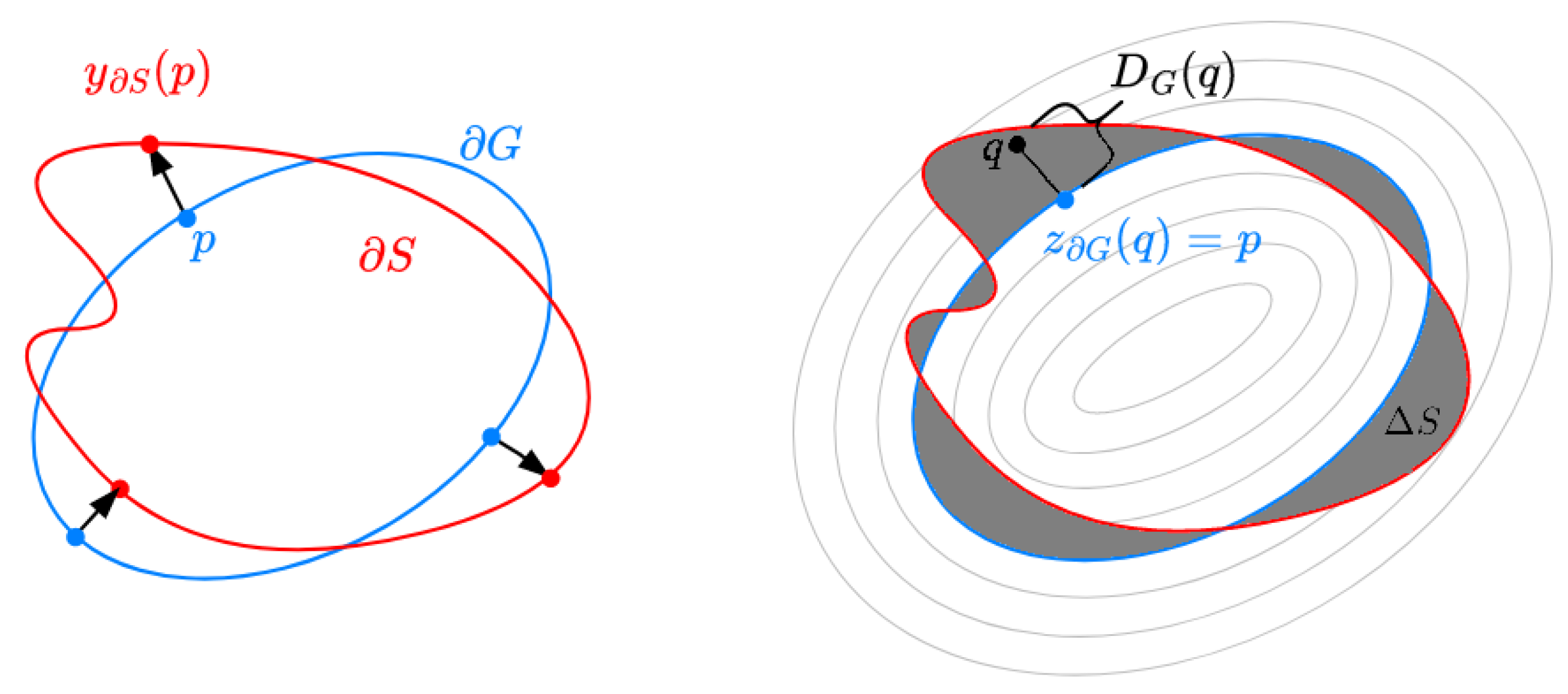
2.3.4. Boundary Loss

The idea behind boundary losses is to penalize the model for incorrect predictions along the boundaries between the prediction and the ground truth.

Boundary loss is inspired by curve evaluation methods [19], which require a measure for evaluating boundary changes. Here, a non-symmetric $L_2$ distance on the space shapes is used that gives a measure of the change between the boundaries $\partial G$ and $\partial S$: i.e., the change between the ground truth and segmentation output boundary, which is defined as

$$Dist(\partial G,\partial S_{\theta })={\int }_{\partial G}{\Vert y_{\partial S}\left(p\right)-p\Vert }^{2}dp$$

(10)

where $\Vert ·\Vert$ denotes the $L_2$ norm, $p\in \Omega$ is a point on the boundary $\partial G$, and $y_{\partial S}\left(p\right)$ denotes the corresponding point on boundary $\partial S$ perpendicular to $\partial G$ at point p. For details, please see Figure 1.

Figure 1. Differential (left) and integral (right) approach for measuring boundary change [20].

By using the integral approach, the need for local differential computation for the contour points is avoided and instead represents boundary changes as a regional integral as follows

$$Dist(\partial G,\partial S)\approx 2{\int }_{\Delta S}{D}_G\left(q\right)dq$$

(11)

where $\Delta S$ denotes the region between the two contours. $D_G:\Omega ⟶{\mathbb{R}}^{+}$ denotes the distance map with respect to the boundary $\partial G$. The distance $D_G\left(q\right)$ for any point $q\in \Omega$ is calculated by taking the closest contour point $z_{\partial G}\left(q\right)=p$ on the boundary $\partial G\left(p\right)$ such that $D_G\left(q\right)=\Vert q-z_{\partial G}\left(q\right)\Vert$. For further information, please see the study by Kervadec et al. [20].

In Figure 1, an illustration of the differential and integral approaches is shown.

The final boundary loss that approximates the boundary distance $Dist(\partial G,\partial S_{\theta })$ is defined as

$${\mathcal{L}}_B\left(\theta \right)={\int }_{\Omega }{\varphi }_G\left(q\right)s_{\theta }\left(q\right)dq$$

(12)

where ${\varphi }_G:\Omega ⟶\mathbb{R}$ denotes the level set function of the boundary $\partial G$ where for a point $q\in G$, ${\varphi }_G\left(q\right)=-D_G\left(q\right)$, and ${\varphi }_G\left(q\right)=D_G\left(q\right)$ otherwise. The term $s_{\theta }\left(q\right)$ denotes the softmax probability outputs.

2.3.5. Dice–BCE Loss

A type of combination loss used with the study by Zhou et al. [10] is the combination between Dice loss and Binary Cross Entropy. This combination loss is described as

$${\mathcal{L}}_{Dice+BCE}(Y,\widehat{Y})={\displaystyle \frac{1}{N}}\sum _{i=1}^N\left({\displaystyle \frac{1}{2}}·Y_i·log{\widehat{Y}}_i+{\displaystyle \frac{2·Y_i·{\widehat{Y}}_i}{Y_i·{\widehat{Y}}_i}}\right)$$

(13)

where N is the batch size and $Y_i$ and ${\widehat{Y}}_i$ are the predicted probabilities and the ground truth, respectively.

2.3.6. Dice–Boundary Loss

Another type of combination loss is the Dice–Boundary Loss, which combines Dice Loss and the Boundary Loss [20]. Boundary loss is suggested as a method for mitigating issues related to regional losses (such as Dice Loss) in cases of highly unbalanced segmentation. As most regional losses penalize all points within a region equally regardless of the distance from the boundary, it can be difficult for regional losses to fit the predictions to the ground truth regions, particularly for small regions. As such, the boundary loss combined with the regional loss can alleviate this potential problem. The combination of dice loss and boundary loss is formulated as

$${\mathcal{L}}_{Dice}+{\mathcal{L}}_B.$$

(14)

In the study by Kervadec et al. [20], three strategies on the weighting of the regional and the boundary loss are proposed by defining the parameter denoted as $\alpha$. The first strategy, called constant, involves setting the parameter to a constant $\alpha =n$, where the total loss is given as

$${\mathcal{L}}_{Dice}+\alpha {\mathcal{L}}_B.$$

(15)

The second approach, called increase, involves setting $\alpha >0$ to a low value and increasing it every i iterations. In this approach, the regional loss remains constant, while the contribution of the boundary loss increases with every iteration.

The third strategy, called rebalance, is defined as

$$(1-\alpha ){\mathcal{L}}_{Dice}+\alpha {\mathcal{L}}_B,$$

(16)

where for a low value of $\alpha >0$, the regional loss is given more importance at the beginning and less with every iteration, while the boundary loss is prioritized more with every iteration.

2.4. Data Augmentation

Data augmentation is a common technique used during the training of deep learning models and aims to increase model generalization (avoid over-fitting) and increase performance on unseen data samples [21,22].

In this study, two categories of image augmentation are employed: image-level and object-level augmentation.

Image-Level Augmentation

Augmentation at the image-level is the most common and easiest implemented form of augmentation [23]. With image-level augmentation, the transform is applied to the whole image and can involve transforms such as flipping, cropping, blurring, contrast adjustment, resizing, cropping, and more. In this study, we used: horizontal flip, vertical flip, and contrast adjustment for image-level augmentation.

2.5. Object-Level Augmentation

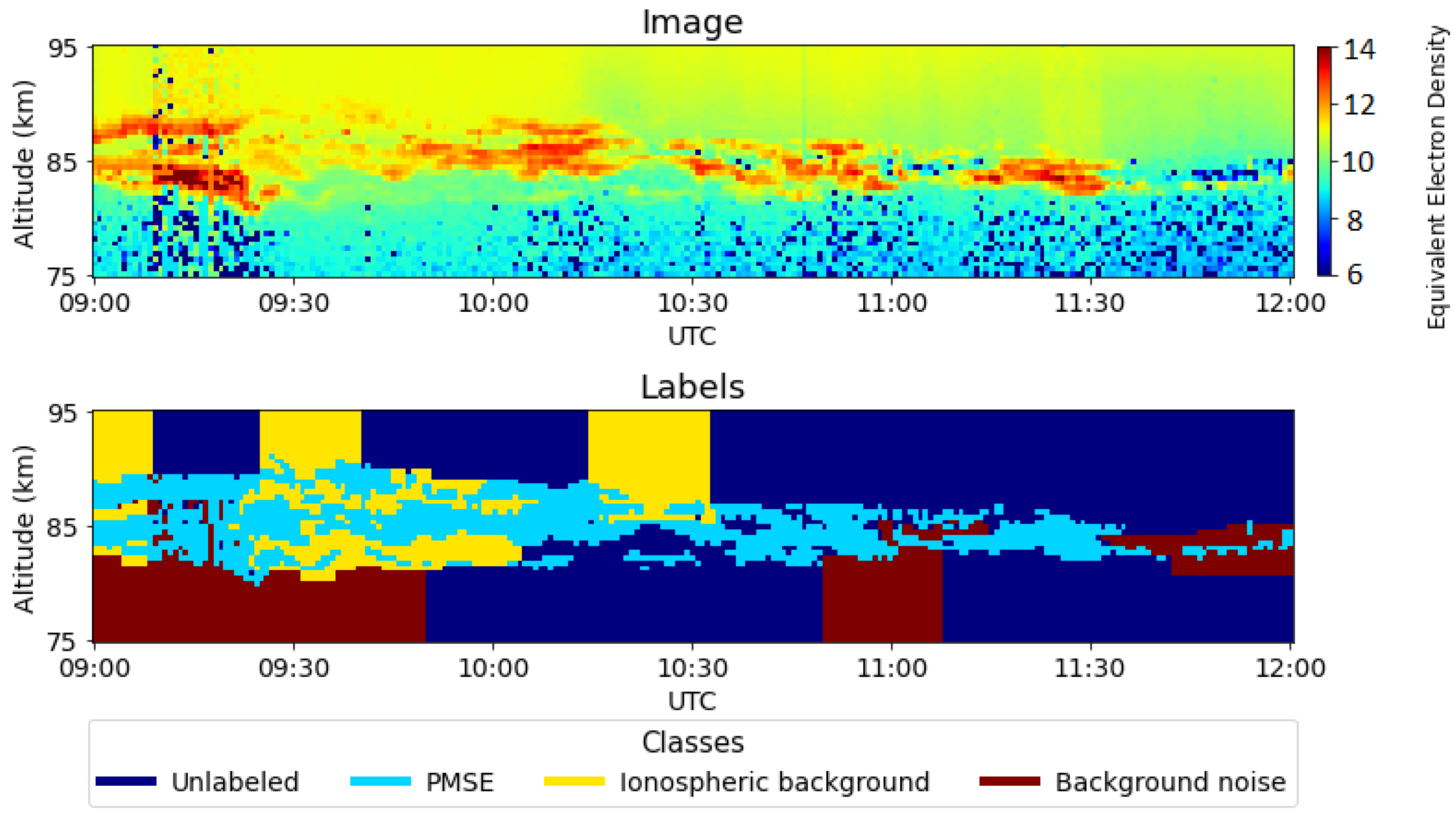
With object-level augmentation, the transforms are applied to the objects that are present in the image. This is a more complex task than the image-level augmentation and requires that the individual target objects be separated from the background and the regions of the image where the objects were removed from to be filled in to avoid artifacts. In this study, an object-level augmentation method called ObjectAug [22] is employed.

ObjectAug [22] is an augmentation method that works at the object-level to generate new samples. The method is defined by the four modules: image parsing, object augmentation, background inpainting, and assemble. Image parsing separates the objects from the rest of the image using the ground truth label, leaving the image with holed-out areas. Then in parallel, the holed-out areas in the image are inpainted, and various data augmentation techniques are performed on individual objects. And last, the objects are placed back in the inpainted image.

3. Data

In this study, we use a dataset from the EISCAT VHF (Very High Frequency, 224 MHz) radar located near Tromsø in Norway. The data include observations of polar mesospheric summer echoes (PMSE) and ionospheric incoherent scatter signals detected during the Arctic summer months in the altitudes of 80 to 90 km [1]. For recent investigation of PMSE with EISCAT observations, we refer the reader to other works [4,5]. The data set used and the data extraction are described in a study by Jozwicki et al. [8].

Each sample in the dataset is a grayscale image containing measured backscatter power. Each image in the dataset is from one observation that typically lasts from a few to several hours with an altitude from 70 to 95 km. The resolution is 0.30 to 0.45 km for the altitude and approximately one minute for the time component [8]. The dataset consists of 18 labeled samples of various sizes, where each sample is a grayscale image. The grayscale images are represented as heatmaps, similar to the study by Jozwicki et al. [8]. In the top image in Figure 2, one of the samples in the dataset is shown, wherein a pixel value refers to the equivalent electron density from the standard GUISDAP analysis [24] and wherein the maximum and minimum values are given in red and blue, respectively. From this, we get 18 data samples containing PMSE associated with 18 different days.

Figure 2. Example of a PMSE image with the ground truth labels [8]. The altitude range is [75, 95] km and the time duration is from 09:00 to 12:00 UTC. The color scale in the image represents equivalent electron density. The labels are divided into Unlabeled (represented by dark blue), PMSE (represented by cyan), Ionospheric Background (yellow), and Background Noise (red). For more details, please see the study by Jozwicki et al. [8].

The original dataset has three different classes: namely, PMSE, background noise, and ionospheric background [8] (see the bottom image in Figure 2). For more information on labeling of image data, please see the study by Jozwicki et al. [8]. In this paper, to simplify the process of segmenting PMSE, we merge the classes, ionospheric background, and background noise with unlabeled classes into one, which is called ’background’. This makes the segmentation process binary. It does, however, create a significant class imbalance between the foreground (PMSE) and the background pixels, with a global ratio of approximately 1:9 between the PMSE and the background, respectively. But it varies a lot between samples and is as low as 1:138 for the sample with the highest class imbalance.

3.1. Constructing Samples from Data

To make the samples compatible with a batch learning scheme and to be used for training a deep learning model, each sample is divided into square patches that are zero-padded on each side to make a sample of size 64 by 64 pixels. The samples in the dataset have four different altitude resolutions: 22, 48, 58, and 60. The samples with a height of 22 pixels are first resized to 44 by 44 pixels using nearest neighbor interpolation and then zero-padded to 64 by 64 pixels. The intention behind scaling up the samples with the smallest altitude resolution is to make them similar to the shape of the other samples, as all samples are in the 75 to 95 km altitude range. In the end, the dataset has 180 image samples extracted from 18 different days of PMSE data.

The dataset is split into training, validation, and test sets and is stratified with the ratio 60%/20%/20%, respectively. The training samples are additionally split such that they overlap by 30%. The data samples are normalized into a float value in the range [0, 1]; after that, the training dataset is normalized to zero mean and unit variance.

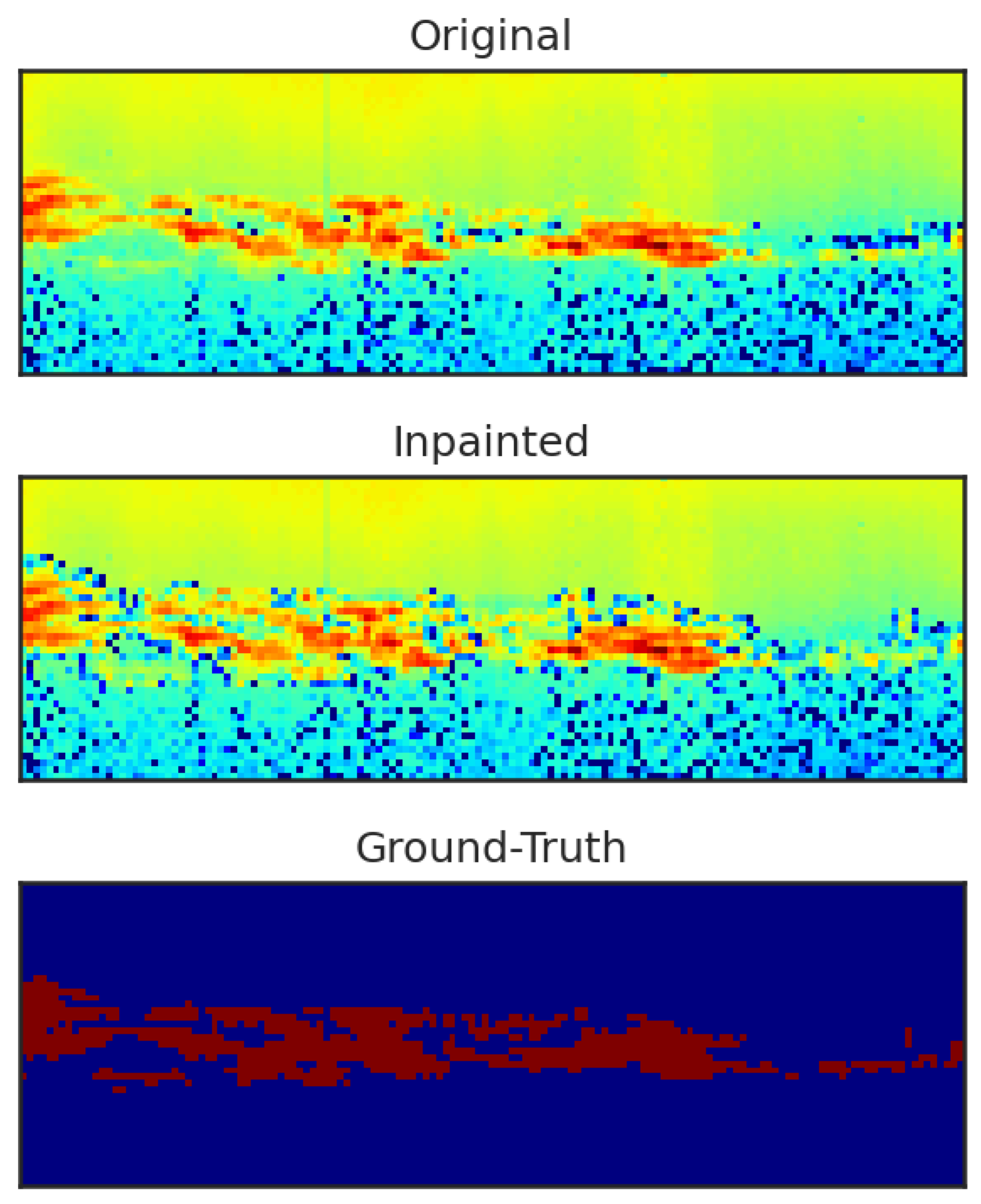
3.2. Data Augmentation Procedure

In order to diversify the original dataset (180 images), the ObjectAug [22] method is employed. We employ inpainting DNN by [25] to fill the removed areas of the image. To avoid any bias between the training of the segmentation models and the inpainting model, the dataset is flipped such that the segmentation training set acts as the validation set and the test for the inpainting model and vice versa for the segmentation test and validation set.

The masks used to train the inpainting model are generated by creating k rectangular patches—denoted as ${\mathbf{M}}_p^k\in {\{0,1\}}^{W\times H}$—of random widths W in the range [1, 20] and heights H in the range [1, 10]. The height and width interval is chosen based on the fact that the majority of the PMSE signal occurrences have a higher width than height. The number of rectangular patches n is chosen to avoid removing large image regions. This is in line with the study by Liu et al. [25] that implies that inpainting large regions is difficult and may lead to bad results. The number of rectangular patches in a mask is set to a value k that is based on the size of the PMSE sample as follows

$$k={\displaystyle \frac{W\times H}{200}}$$

(17)

where the denominator is found based on visual inspection. By changing the number of patches as a function of image size, we avoid removing regions that are too big or too small.

The rectangular patches are randomly placed in the PMSE mask such that the rectangular patches and PMSE mask do not overlap. This facilitates the model to avoid learning the PMSE signal. The different patches are then assembled into one mask. For each of the 18 PMSE samples, 50 different inpainting masks are generated.

For the training of the inpainting DNN, a UNet architecture is used with the same depth as the UNet model [9] and uses ResNet50 [26] trained on ImageNet [27] as the backbone. The same loss from [25] is used with the Adam optimizer algorithm with a learning rate of 0.0005. The model is trained for 10,000 iterations with a mini-batch size of 32.

For ObjectAug’s image parsing module [22], the PMSE regions defined by the ground truth are extracted from the image. We define a PMSE region as an individual region if there is more than one background pixel separating the boundaries of the regions. This small distance between regions is selected because the number of PMSE regions decreases drastically if the distance is set higher.

For the Object Augmentation module, resizing and location shifts are applied as the augmentation methods, with each having a probability of $p=0.5$ of being invoked.

For the resizing augmentation, the scaling of the PMSE region is based on a random number denoted as $n\in [-3,3]$, where the n corresponds to the number of pixels by which the object is scaled down or scaled up. The reason that the objects are only scaled up or down by a few pixels is to avoid PMSE regions either becoming too big—i.e., the PMSE stretches into regions of other PMSE—or outside the 80 to 90 km altitude range of PMSE.

For the location shift augmentation, the PMSE region is shifted horizontally and/or vertically. The number of pixel points by which the objects are shifted is randomly selected in the range $[-3,3]$ for both the horizontal and vertical shifts. The shifting range is limited to only a few pixels to avoid PMSE regions overlapping or being shifted outside of the 80 to 90 km altitude range.

After augmenting the individual PMSE regions, they are placed back into the image in the Assemble module [22]. Object augmentation [22] is a computationally heavy process. Therefore, to speed up training, the object augmented data used during training are pre-computed. This generates 900 new image samples. In addition to the 900 new samples, we include 180 samples of the original dataset such that 20 percent of the total samples are not augmented. This is because the inpainted images create a different background around the PMSE, and by adding the un-augmented samples, the data will also contain natural boundaries between the foreground, i.e., PMSE, and the background.

4. Model Hyperparameters

In the experiments, two different UNet architectures, i.e., UNET and UNET++, are used. Given that our task is binary, sigmoid activation is used to produce the final output. The number of initial feature maps is set to 32 or 64, and the architectures are represented as UNet${}^{32}$ or UNet${}^{64}$.

Both randomly initiated weights and pre-trained weights are used during the experiments. In the latter case, the pre-trained weights are only used in the encoder layers. The remaining layers are initiated using Kaiming He [28] initialization. In the randomly initiated case, all layers are initiated using Kaiming He initialization.

For all experiments, the Adam optimizer algorithm [29] is employed with ${\beta }_1=0.9$ and ${\beta }_2=0.999$, which is suggested as a good starting point in the Adam paper [29]. To avoid overfitting, an early stopping mechanism is used, similar to that of Algorithm 7.1 in [30], where the best parameters, denoted with ${\theta }^{*}$, are selected based on the validation error. Depending on if the data are augmented, the patience p is set to a different value. For the models using no augmentation, $p=10$, and for the models using augmentation, $p=20$. For the latter case, the patience is set higher because the validation error is more irregular during training. The models are evaluated every 10 iterations using a mini-batch size of eight randomly selected samples and run until the early stopping criteria are met. The models are trained on an Nvidia RTX3070 (notebook) GPU with 8 GB of VRAM.

5. Results

In this section, we briefly discuss the different experiments and the associated results.

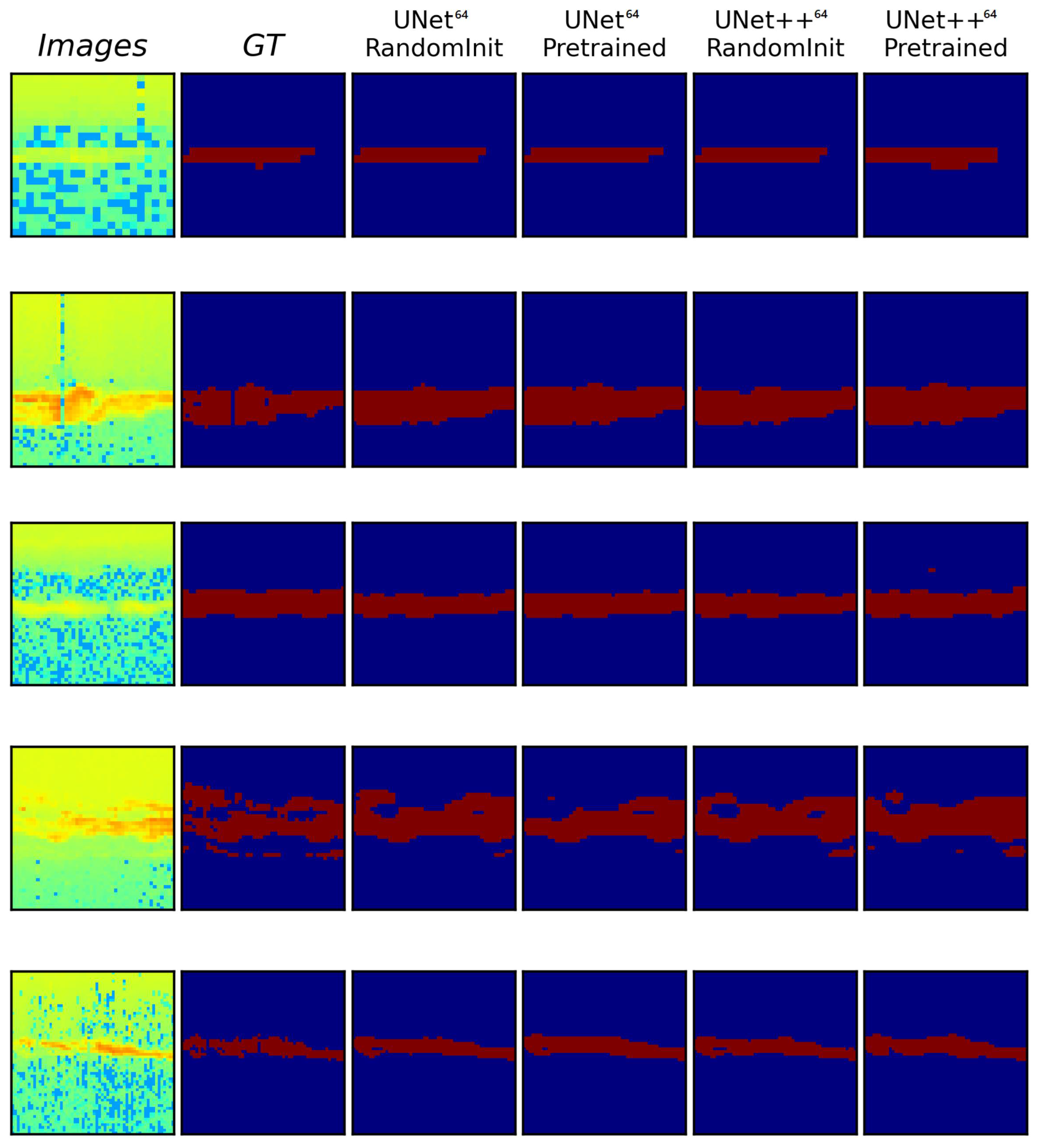
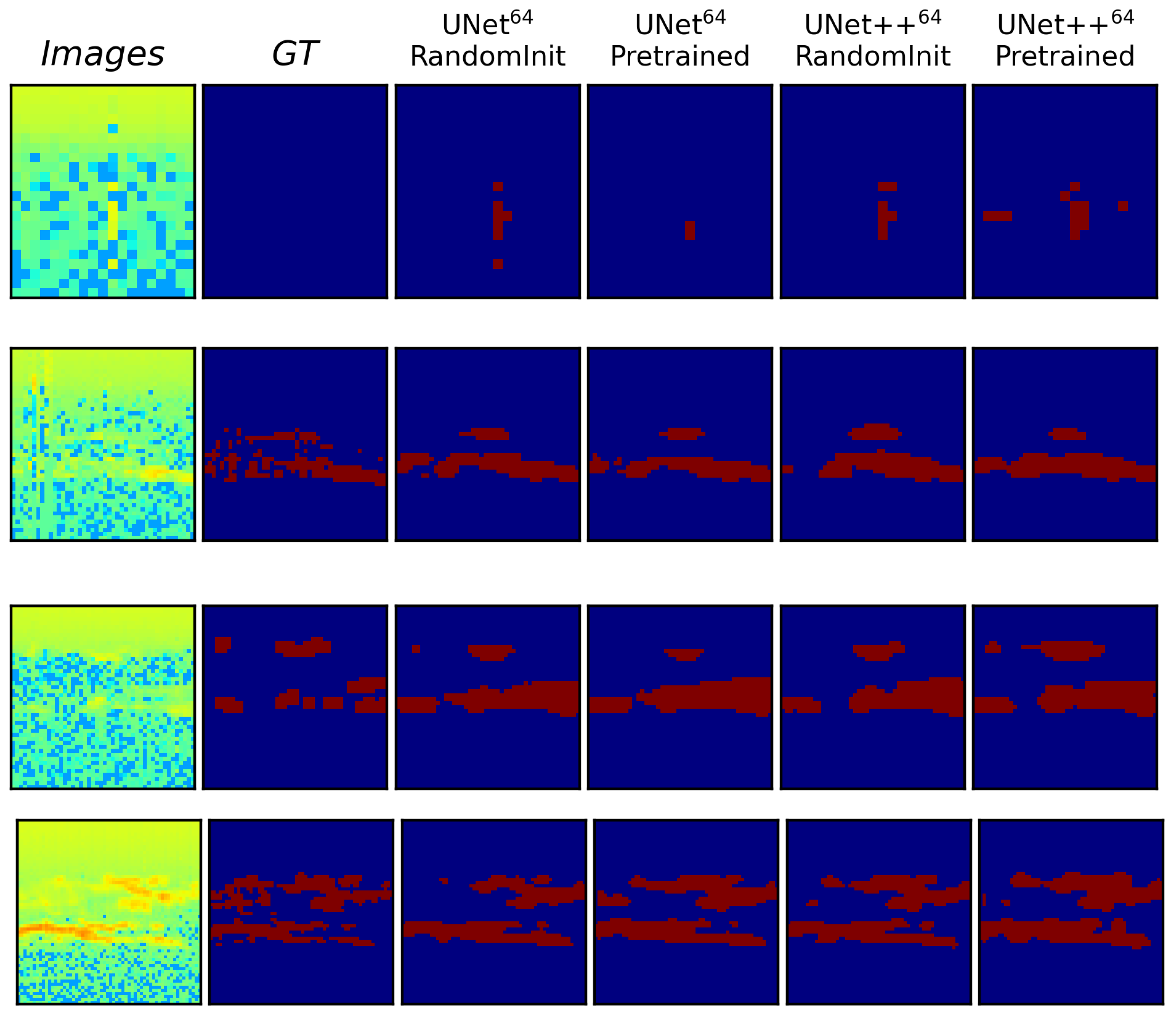
5.1. Initial Experiment

Initially, a set of experiments is conducted using UNet [9] and UNet++ [10] using the original dataset. Based on the two architectures, we test eight models, applying different variations as follows:

• Randomly initiated weights with 32 and 64 initial feature maps.
• Pretrained weight initiation of the encoder layers. For the models with 32 initial feature maps, a pretrained UNet model found at (Note: https://pytorch.org/hub/mateuszbuda_brain-segmentation-pytorch_unet, accessed on 14 August 2023) is used. For the models with 64 initial feature maps, a VGG16 [31] model pretrained on ImageNet [27] is used as the backbone.

A random hyperparameter search is run for the experiments with random learning rates and weight decays in the range $[0.01,0.0001]$. For details, please see Table 1, where the learning rates and weight decays for the different models and different hyperparameters are shown. The selection of parameters is done based on the highest Dice–Sørensen coefficient score where the loss is reasonably stable and where the difference between the training and validation score is not high.

Table 1. Learning rate and weight decay values used during training of the different models listed in Table 2. The values selected are based on the hyperparameter search.

Model–Initiation	Hyperparameters
	Learning Rate	Weight Decay
UNet${}^{32}$–RandomInit	0.008	0.005
UNet${}^{32}$–Pretrained	0.003	0.007
UNet${}^{64}$–RandomInit	0.006	0.005
UNet${}^{64}$–Pretrained	0.003	0.007
UNet++${}^{32}$–RandomInit	0.005	0.005
UNet++${}^{32}$–Pretrained	0.003	0.006
UNet++${}^{64}$–RandomInit	0.002	0.006
UNet++${}^{64}$–Pretrained	0.001	0.008

UNet${}^{32}$ denotes 32 initial feature maps and UNet${}^{64}$ denotes 64 initial feature maps in the first convolutional layer.

For each model or model with a selected hyperparameter, the training, validation, and testing data are randomly selected. This step is repeated five times, and to calculate the performance, we use the mean and standard deviations of the scores from five repetitions of the same experiment. The quantitative results from the initial experiment (in Table 2) show the IoU and DSC scores on the test and validation datasets.

Table 2. Quantitative performance of different UNet architectures with 32 or 64 initial feature maps. IoUs and DSCs are reported for the test and validation sets. The best-performing model is underlined.

Model–Weight Initiation	Test		Validation
	IoU	DSC	IoU	DSC
UNet${}^{32}$–RandomInit	0.654 ± 0.006	0.791 ± 0.005	0.710 ± 0.007	0.830 ± 0.005
UNet${}^{32}$–Pretrained	0.634 ± 0.010	0.776 ± 0.007	0.699 ± 0.008	0.823 ± 0.006
UNet${}^{64}$–RandomInit	0.649 ± 0.005	0.787 ± 0.003	0.713 ± 0.011	0.832 ± 0.008
UNet${}^{64}$–Pretrained	0.645 ± 0.005	0.784 ± 0.004	0.702 ± 0.005	0.825 ± 0.003
UNet++${}^{32}$–RandomInit	0.654 ± 0.012	0.790 ± 0.008	0.713 ± 0.005	0.833 ± 0.003
UNet++${}^{32}$–Pretrained	0.632 ± 0.027	0.774 ± 0.021	0.692 ± 0.030	0.817 ± 0.021
UNet++${}^{64}$–RandomInit	0.666 ± 0.010	0.799 ± 0.007	0.727 ± 0.008	0.842 ± 0.005
UNet++${}^{64}$–Pretrained	0.649 ± 0.006	0.787 ± 0.004	0.719 ± 0.008	0.837 ± 0.005

UNet${}^{32}$ and UNet${}^{64}$ denote 32 and 64 initial feature maps, respectively, in the first convolutional layer.

The best results are underlined. The results indicate that there are minor differences between the performance of the different models and between models with different hyperparameters. However, the best-performing model—i.e., UNet++${}^{64}$ with randomly initiated weights—has relatively better performance compared to the other models considered. From Table 2, we can observe that for the same model architectures and sizes—i.e., the number of initial feature maps—the model that uses pre-trained weight in the encoder layers performs worse than the randomly initiated model.

To better visualize where the models perform well and where they struggle, a few selected samples from the test set are included in Figure 3 and Figure 4, which show samples or cases that are easy and difficult, respectively. Here, the easy samples are defined as the cases for which the predicted regions are closer to the ground truth, and difficult samples are defined as the cases for which the predictions are different from those of the ground truth. In each of the figures, the first column represents the image, the second column shows the ground truth, and the next four columns show the predictions from the four models: UNet${}^{64}$—Pretrained, UNet${}^{64}$—RandomInit, UNet++${}^{64}$—RandomInit, and UNet++${}^{64}$—Pretrained, respectively.

Figure 3. Easy samples: Qualitative comparison between UNet${}^{64}$–RandomInit, UNet${}^{64}$–Pretrained, and UNet++${}^{64}$–RandomInit showing some of the test samples for which the predicted regions are closer to the ground truth. The images and their ground truth labels are shown in the first and second columns, respectively.

Figure 4. Difficult Samples: Qualitative comparison between UNet${}^{64}$–RandomInit, UNet${}^{64}$–Pretrained, and UNet++${}^{64}$–RandomInit showing some of the test samples for which the predicted regions are different than the ground truth. The images and their ground truth labels are shown in the first and second columns, respectively.

From the easier samples in Figure 3, it seems that all models used in the experiments segment the PMSE regions accurately and that the predictions are quite similar between the different models.

Now we examine the more-challenging data samples in Figure 4. For instance, the first-row image has an empty foreground: i.e., there is no PMSE, but the models predict PMSE. Upon inspection of the PMSE predictions, we observe that the small regions predicted as PMSE have slightly higher values than those in their neighborhoods. A similar trend is observed with other images in rows 2, 3, and 4, where the models predict larger regions of PMSE as compared to the ground truth.

In order to see if there is any significant difference between the pretrained models with respect to important features in the input images, relevance maps are generated using the LRP method from the study by Montavon et al. [32].

In Figure 5, we can see the input images, their ground truth maps, and relevance maps for the different models with different pretrained weights. There is visually little difference between the models with pretrained weights from the different source domains. Rather, the difference in relevance can be linked to the type of model architecture used.

Figure 5. The figure shows the explained relevance produced using four different models using pretrained weights in the encoder. UNet${}^{32}$/UNet++${}^{32}$ use pretrained weights from the medical image domain, and UNet${}^{64}$/UNet++${}^{64}$ use pretrained weights from the image domain. In the first and second columns, the images and ground truth are shown, respectively. The values of the relevance maps are centered around 0.5 (black), which indicates no relevance. Full relevance is given a value of 1 (white), while inverse relevance is assigned a value of 0 (cyan).

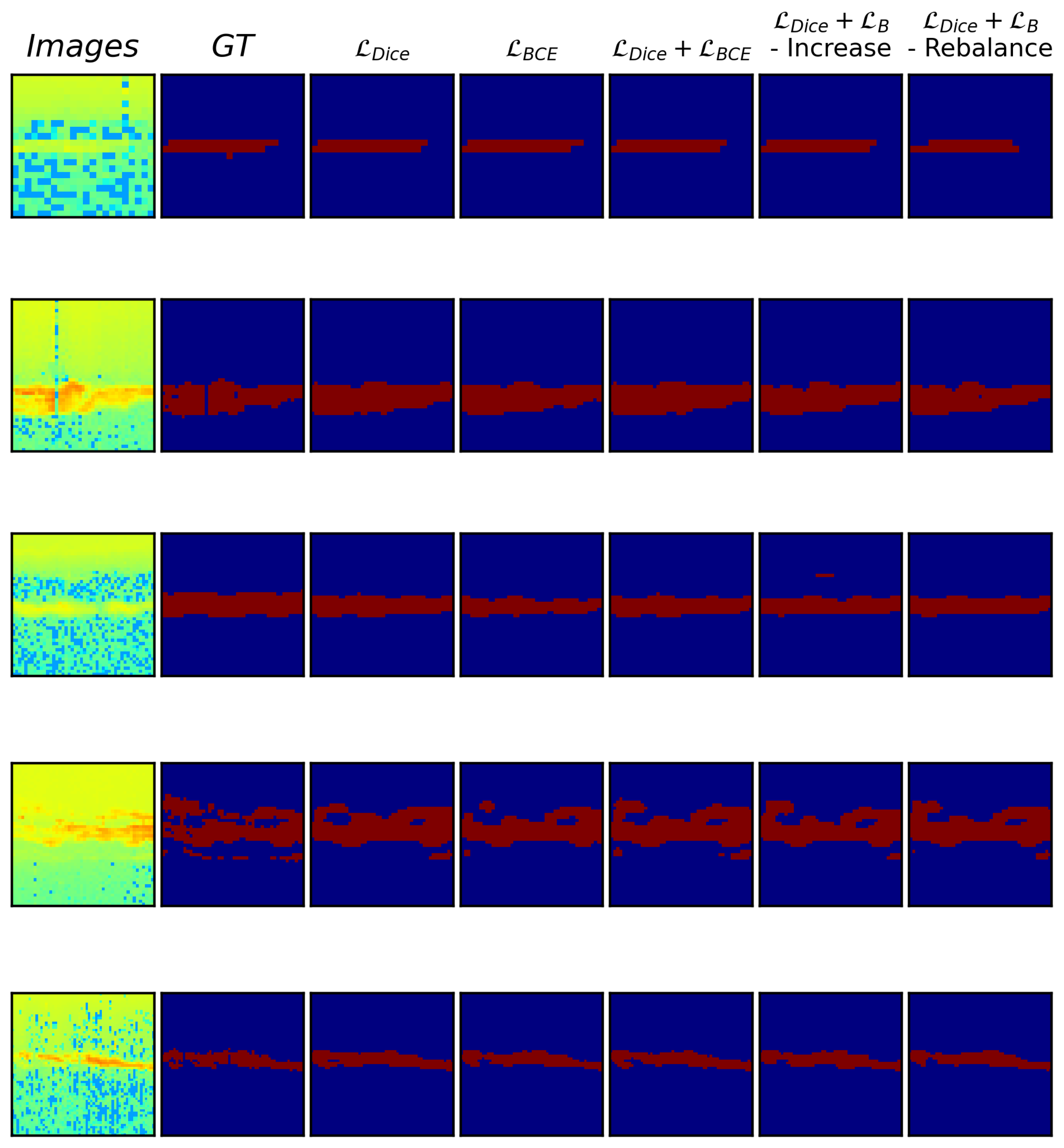
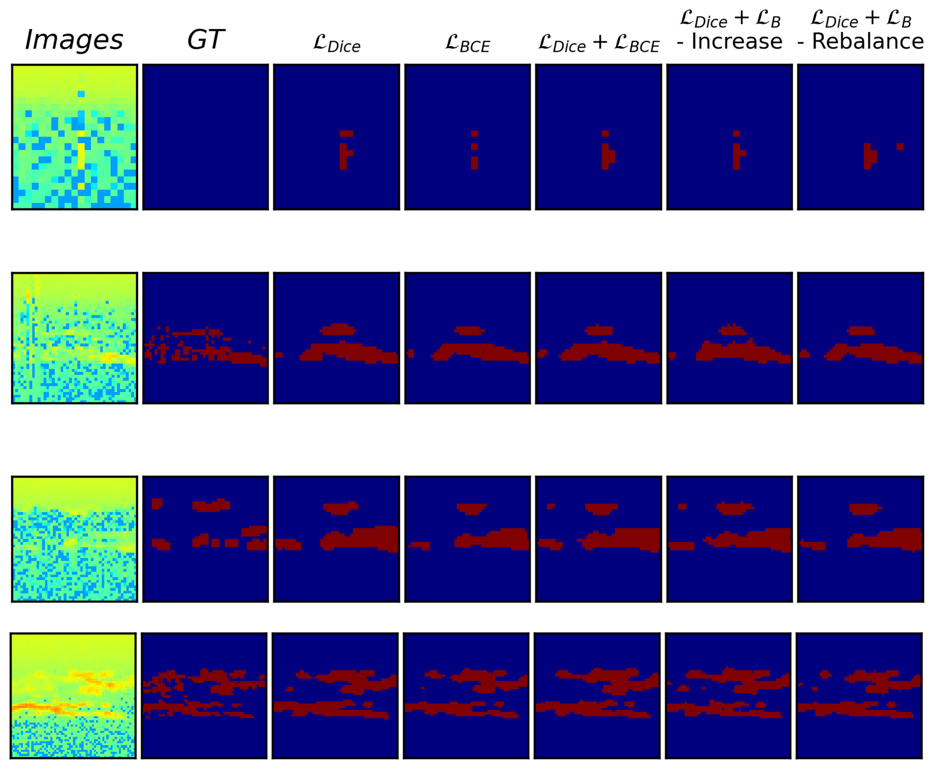
5.2. Using Different Loss Functions

Building on the results from the initial experiment, we investigate the impact of different loss functions on performance. For these experiments, the randomly initiated UNet++${}^{64}$ model that had the best performance in the initial experiment in Section 5.1) is used as a baseline. For comparison, the same model is trained with the four other loss functions; Binary Cross Entropy (BCE), Focal Loss, Dice–BCE Loss, and Dice–Boundary Loss, denoted as ${\mathcal{L}}_{BCE}$, ${\mathcal{L}}_{Focal}$, ${\mathcal{L}}_{Dice}+{\mathcal{L}}_{BCE}$ and ${\mathcal{L}}_{Dice}+{\mathcal{L}}_B$, respectively.

For ${\mathcal{L}}_{Focal}$ and ${\mathcal{L}}_{Dice}+{\mathcal{L}}_B$, parameters are specified as follows:

• ${\mathcal{L}}_{Focal}$: $\gamma =2.0$ is set equal to that of thr original paper [18], while $\alpha =0.8$ is chosen such that it is approximately inversely proportional to the foreground frequency.
• ${\mathcal{L}}_{Dice}+{\mathcal{L}}_B$: the increase and rebalance schedule strategies [20] for setting $\alpha$ are used:

  –

  Increase: For the increase schedule, $\alpha =0.01$ initially, and it is increased by $0.01$ every five iterations, where $\alpha =max(\alpha ,1)$.

  –

  Rebalance: For the Rebalance, $\alpha =0.005$ initially and follows a schedule based on the number of iterations as follows

  $$\alpha =\left\{\begin{array}{cc}\alpha +0.005,\hfill & \mathrm{if}iter<100\hfill \\ \alpha +0.01,\hfill & \mathrm{if}100\le iter<300\hfill \\ \alpha +0.02,\hfill & \mathrm{otherwise}\hfill \end{array}\right.$$

  (18)

  This is a slightly different scheduling of $\alpha$ than that of the original rebalance strategy [20] and is considered necessary as the model struggles when $\alpha$ is increased too quickly in the start.

When $\alpha$ is dynamically changed during training, a problem can arise where the loss might increase even though the IoU and DSC are improving, thus triggering the stopping criterion prematurely. Because the two losses are measures of different objectives and at the same time are weighted dynamically, the total loss might not follow the typical loss learning curve. As such, the IoU metric is used instead of loss as the stopping criterion.

The quantitative results shown in Table 3 indicate that ${\mathcal{L}}_{Dice}+{\mathcal{L}}_{BCe}$ has the best performance, but it is only slightly better than the loss of ${\mathcal{L}}_{Dice}$ loss. The distribution-based losses such as (${\mathcal{L}}_{BCe}$ and ${\mathcal{L}}_{Focal}$) do not reach the same performance as the regional loss (${\mathcal{L}}_{Dice}$), but, as noted, the combination of ${\mathcal{L}}_{Dice}$ and ${\mathcal{L}}_{BCE}$ gives an increase in performance. When it comes to the combination of ${\mathcal{L}}_{Dice}+{\mathcal{L}}_B$ and the two different scheduling strategies of $\alpha$, the Increase strategy has the best performance.

Table 3. Quantitative performance of a randomly initiated UNet++${}^{64}$ architecture using different loss functions. IoU and DSC are reported for the test and validation sets. The best-performing model is underlined.

Loss Function $\left(\mathcal{L}\right)$	Test		Validation
	IoU	DSC	IoU	DSC
${\mathcal{L}}_{Dice}$	0.666 ± 0.010	0.799 ± 0.007	0.727 ± 0.008	0.842 ± 0.005
${\mathcal{L}}_{BCE}$	0.656 ± 0.006	0.792 ± 0.004	0.714 ± 0.003	0.833 ± 0.002
${\mathcal{L}}_{Focal}$	0.647 ± 0.003	0.786 ± 0.002	0.695 ± 0.002	0.820 ± 0.001
${\mathcal{L}}_{Dice}+{\mathcal{L}}_{BCE}$	0.667 ± 0.005	0.800 ± 0.003	0.731 ± 0.004	0.844 ± 0.003
${\mathcal{L}}_{Dice}+{\mathcal{L}}_B$–Increase	0.662 ± 0.013	0.797 ± 0.010	0.722 ± 0.011	0.838 ± 0.007
${\mathcal{L}}_{Dice}+{\mathcal{L}}_B$–Rebalance	0.650 ± 0.011	0.788 ± 0.008	0.703 ± 0.012	0.825 ± 0.008

${\mathcal{L}}_{dice}+{\mathcal{L}}_B$ is denoted with either the Increase or Rebalance schedule.

A visualization of the predictions made by the models trained with the different loss functions is shown in Figure 6 and Figure 7 for the easy and difficult samples, respectively.

Figure 6. Easy Samples: Qualitative comparison between the different loss functions ${\mathcal{L}}_{Dice}$, ${\mathcal{L}}_{BCE}$, ${\mathcal{L}}_{Dice}+{\mathcal{L}}_{BCE}$, and ${\mathcal{L}}_{Dice}+{\mathcal{L}}_B$ (Increase or Rebalance scheduling) using a randomly initiated UNet++${}^{64}$ architecture. The images and their ground truth labels are shown in the first and second columns, respectively.

Figure 7. Difficult Samples: Qualitative comparison between the different loss functions ${\mathcal{L}}_{Dice}$, ${\mathcal{L}}_{BCE}$, ${\mathcal{L}}_{Dice}+{\mathcal{L}}_{BCE}$, and ${\mathcal{L}}_{Dice}+{\mathcal{L}}_B$ (Increase or Rebalance scheduling) using a randomly initiated UNet++${}^{64}$ architecture. The images and their ground truth labels are shown in the first and second columns, respectively.

For both the easy and difficult samples, it can be seen that there are differences between the segmented regions depending on the loss function used. Looking at the single loss functions (${\mathcal{L}}_{Dice}$, ${\mathcal{L}}_{BCE}$, and ${\mathcal{L}}_{Focal}$), the model trained with ${\mathcal{L}}_{Dice}$ seems to segment larger regions than that of the distributions based ${\mathcal{L}}_{BCE}$ and ${\mathcal{L}}_{Focal}$, which have narrower predicted regions. The two models that use combination losses (${\mathcal{L}}_{Dice}+{\mathcal{L}}_{BCE}$ and ${\mathcal{L}}_{Dice}+{\mathcal{L}}_B$) have quite similar segmented regions and still predict PMSE regions where no PMSE is present (please see Figure 7, first row).

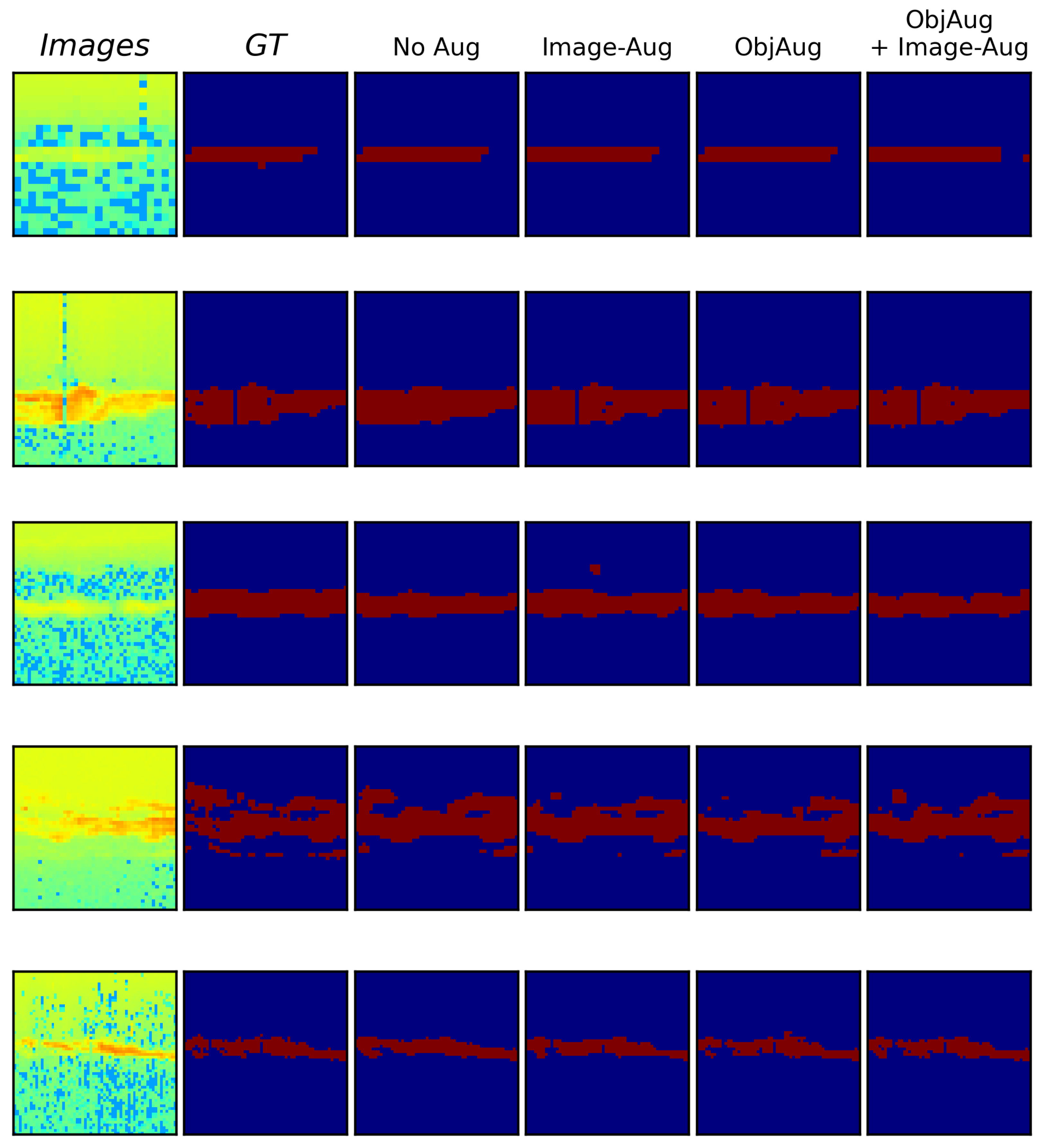
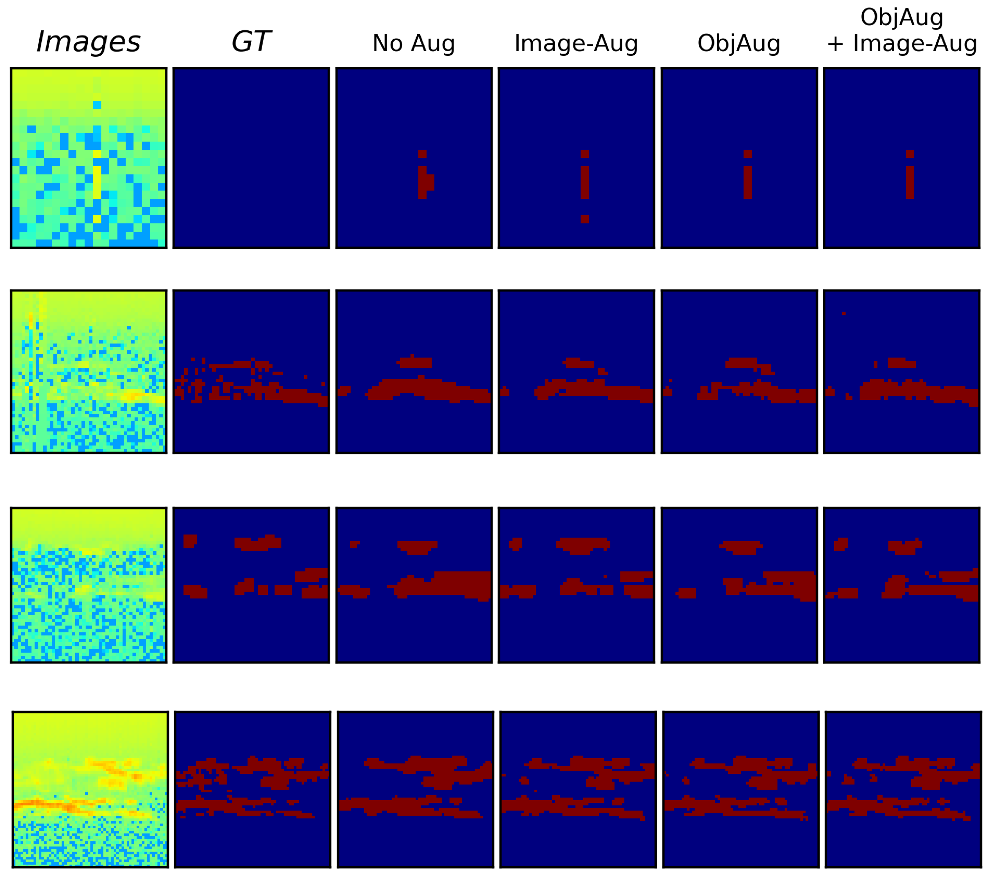
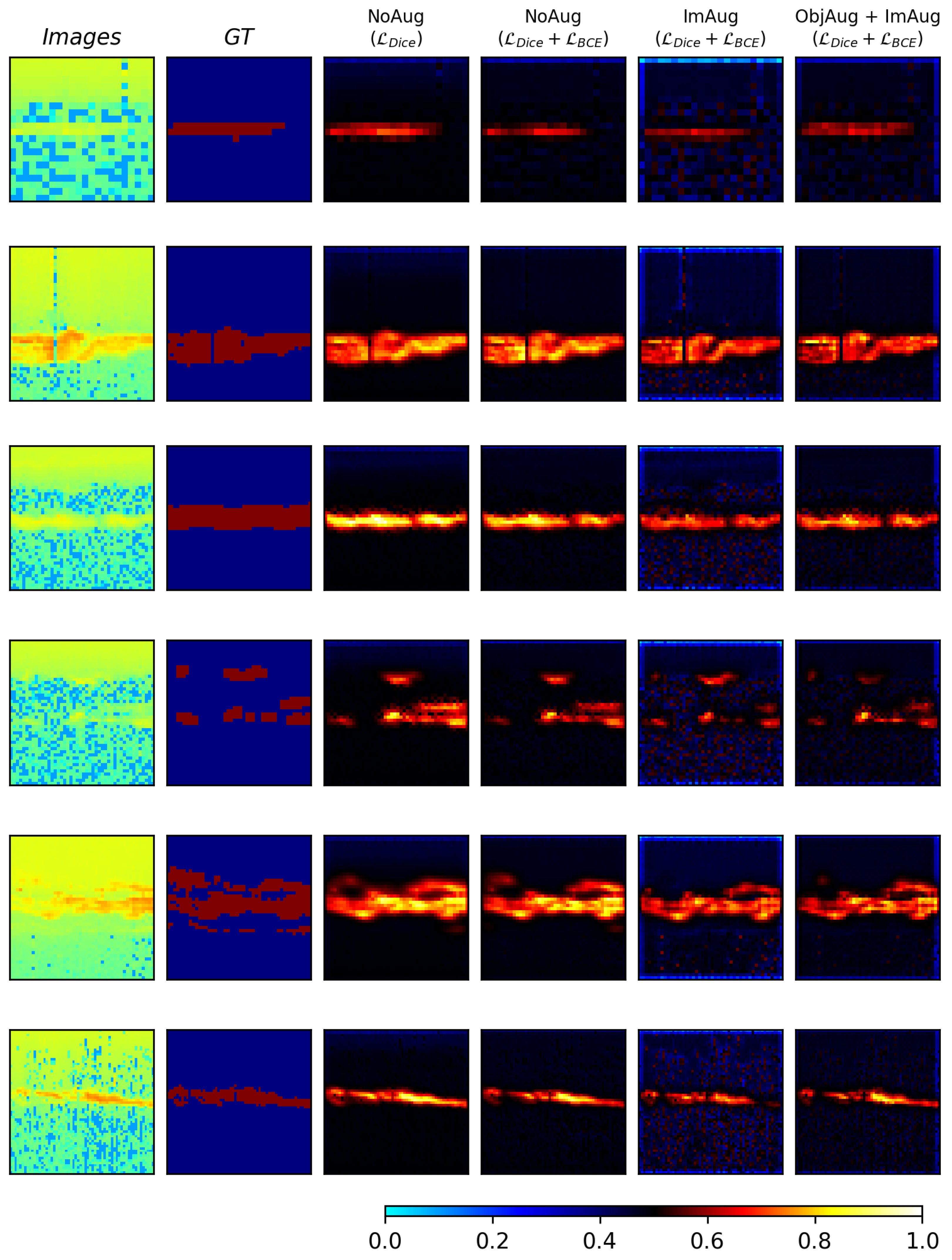
5.3. Using Image-Level and Object-Level Augmentations

Following the results from the previous section, the UNet++${}^{64}$ model with randomly initiated weights and ${\mathcal{L}}_{Dice}+{\mathcal{L}}_{BCE}$ loss is used as a baseline for these experiments.

To see the effect that simple image-level augmentation can have on performance, five experiments are conducted. Image augmentation techniques such as horizontal flip, vertical flip, and contrast adjustment and their combinations are used in the experiments. A probability of $p=0.5$ of invoking the augmentation method is used. For the contrast adjustment method, the adjustment factor C is randomly chosen from the interval $C\in [0.8,1.2]$.

The results are shown in Table 4 and indicate that applying all the augmentation techniques individually increases performance compared to the baseline, i.e., no augmentation. When all the individual augmentation techniques are combined, the increase in performance is only slightly better than that of the baseline. In the last row of Table 4, it can be observed that for the test dataset when using both horizontal flip and contrast adjustment augmentation, there is improvement in performance as compared to individual image augmentation methods.

Table 4. Quantitative performance using different image-level augmentations separately and combined. IoUs and DSCs are reported for the test and validation sets. The best-performing model is underlined.

Model–Augmentation	Test		Validation
	IoU	DSC	IoU	DSC
Baseline	0.667 ± 0.005	0.800 ± 0.003	0.731 ± 0.004	0.844 ± 0.003
Horizontal Flip	0.682 ± 0.010	0.811 ± 0.007	0.742 ± 0.008	0.851 ± 0.005
Vertical Flip	0.672 ± 0.006	0.804 ± 0.004	0.739 ± 0.009	0.849 ± 0.006
Contrast Adjust	0.683 ± 0.005	0.811 ± 0.003	0.742 ± 0.002	0.851 ± 0.001
All Combined	0.669 ± 0.007	0.801 ± 0.005	0.741 ± 0.008	0.851 ± 0.006
Horizontal and Contrast Adjust	0.694 ± 0.008	0.819 ± 0.006	0.735 ± 0.004	0.847 ± 0.003

After image-level augmentation experiments, two more experiments are performed using the object-level augmentation method known as ObjectAug [22]. In the first experiment, we use the object-level [22] method alone, and in the second, we use object-level and image-level augmentation together. Here, for image-level augmentation, we use both horizontal flip and contrast adjustment augmentation based on results from the previous section. The results are shown in Table 5. Here, the baseline model is the same as in Table 4 using no augmentation. Our results indicate that the two models trained on the augmented dataset show improvements compared to the baseline. Between the two models trained using the ObjectAug method, it is clear that additional image-level augmentation improves the performance. However, the performance is only slightly improved compared to only using image-level augmentation.

Table 5. Quantitative performance of using no augmentation and image-level, object-level, and both image-level and object-level augmentation. IoUs and DSCs are reported for the test and validation sets. The best-performing model is underlined.

UNet++${}^{64}$–RandomInit	Test		Validation
	IoU	DSC	IoU	DSC
No Aug	0.667 ± 0.005	0.800 ± 0.003	0.731 ± 0.004	0.844 ± 0.003
Image-Aug	0.694 ± 0.008	0.819 ± 0.006	0.735 ± 0.004	0.847 ± 0.003
ObjAug	0.678 ± 0.009	0.808 ± 0.007	0.719 ± 0.007	0.836 ± 0.005
ObjAug and Image-Aug	0.701 ± 0.010	0.824 ± 0.007	0.730 ± 0.003	0.843 ± 0.002

The model predictions can be seen in Figure 8 and Figure 9 showing the easy and difficult samples, respectively. In Columns 1 and 2 in the figures, the images and ground truths are supplied. Columns 3 to 6 show the predictions from the models that were trained and are shown in Table 5.

Figure 8. Easy Samples: Qualitative comparison between using different types of augmentation using a UNet++${}^{64}$ model with randomly initiated weights. In the first and second columns, the images and ground truth, respectively, are shown. The rest of the columns show the predictions associated with different augmentation methods.

Figure 9. Difficult Samples: Qualitative comparison between using different types of augmentation using a UNet++${}^{64}$ model with randomly initiated weights. In the first and second columns, the images and ground truth, respectively, are shown. The rest of the columns show the predictions associated with different augmentation methods.

The results in Table 5 imply that when using object-level augmentation, the performance is worse than when using only the image-level horizontal and contrast adjustment augmentation. However, when applying the same image-level augmentation with object-level augmentation, the performance is improved slightly. Although the increase in performance is low, it can be seen in the qualitative results in Figure 8 and Figure 9 that the model that uses object-level augmentation predicts regions in a different way, as it is aware of potential PMSE regions; this is further discussed in Section 6).

6. Discussion

Label inconsistency is a problem for supervised deep learning models that may lead to inaccurate and unreliable results. The labeling of data is strongly influenced by human factors. Data labeled at different times and by different persons can be a contributing factor to label inconsistency. In this study, the data is labeled by one expert using different labeling tools at different times. This is something that can lead to noisy labels. To address this, further validation studies are needed with multiple experts in the loop.

Our results from Section 5.1 indicate that for the same model type—i.e., the same number of initial parameters and architecture—using pretrained weights in the encoder is shown to perform worse than randomly initiated weights. As the pretrained UNet${}^{32}$ and UNet++${}^{32}$ models use weights from the medical imagery domain, and the UNet${}^{64}$ and UNet++${}^{64}$ models use weights from the natural image domain, this implies that different source domains might not be directly applicable to our target domain of PMSE data. From the experiments (described in Section 5.1), we observe that UNet++${}^{64}$ with randomly initiated weights has relatively better performance than the rest of the models used in these experiments.

The results from Section 5.2 indicate that the UNet++${}^{64}$ model with randomly initiated weights for which ${\mathcal{L}}_{Dice}+{\mathcal{L}}_{BCE}$ is used as a loss function performs better compared to the other loss functions used in this paper.

We find that using image-level augmentation improves the performance of the model. These results are in line with other studies [21,22,31] that indicate the positive impact of using image-level augmentation. It should be noted that the data used in this study are different from those of real-world scenes or the medical domain. PMSE regions occur at specific altitude ranges and in shapes that stretch longer horizontally than vertically in the sample images. From Table 4, it can be seen that the vertical flipping of the image does show an improvement in performance compared to using no augmentation. However, it can also be seen from the figure that excluding vertical-flip augmentation from the combined augmentation increases performance. This could possibly indicate that augmentation that changes the PMSE regions in an unnatural way—i.e., rotating or flipping the image such that PMSE and the background occur in places that are not possible—could lead to worse performance.

The results from Section 5.3 imply that the combined effect of image-level and object-level augmentation techniques is better for the overall performance of the proposed UNet++${}^{64}$ model with randomly initiated weights and ${\mathcal{L}}_{Dice}+{\mathcal{L}}_{BCE}$ loss.

It should be noted that employing object-level augmentation for our data can change the boundary between PMSE and the background. The inpainting of images impacts how the model learns the boundary between the background and the PMSE. When the images are inpainted, a slightly bigger region around the PMSE is removed to avoid leftover pixels that might be unlabeled PMSE. However, as illustrated in Figure 10 where augmentation is applied to the PMSE regions, the inpainted region around the PMSE can be quite different from the original. The outcome is that the contrast between PMSE and the inpainted background is often increased, which in turn can influence how the model predicts PMSE regions.

Figure 10. Illustration of the different boundaries between foreground and PMSE that the inpainted image creates compared to the original image.

To better see the difference between using augmentation versus no augmentation, LRP is employed to visualize the features in the input image that are considered relevant for the models. For the models trained using augmentation, it can be seen that the regions that the models consider important are slightly different as compared to the models trained without augmentation. For details, please see Figure 11. The relevance maps from the models trained using augmentation seemingly give an overall lower relevance score as compared to using no augmentation. This might indicate that the models that use no augmentation during training are more biased towards certain areas of the input. This might imply that the models that use augmentation (both image-level and object-level) can perhaps generalize better to unseen cases. This is something that can be explored in future studies when a sufficient amount of data can be obtained.

Figure 11. Relevance maps produced using four different models. All models use a randomly initiated UNet++${}^{64}$ architecture. The type of augmentation and type of loss function used are shown in the columns. ObjAug denotes object-level augmentation, ImAug denotes image-level augmentation, and NoAug denotes that no augmentation was used. In the first and second columns, the images and ground truth, respectively, are shown. The values of the relevance maps are centered around 0.5 (black), which indicates no relevance. Full relevance is given a value of 1 (white), while inverse relevance is assigned a value of 0 (cyan).

We believe that our proposed model can be used for segmenting PMSE from EISCAT VHF data across a much wider range of days from different years of the solar cycle. In the near future, the model proposed in this paper can be used to extract PMSE samples from a potentially large dataset of EISCAT observations. The results of the segmentation can be useful for further in-depth analysis of PMSE and other phenomena pertaining to the upper atmosphere.

7. Conclusions

In this paper, we investigate the possibility of employing fully convolutional networks such as UNET and UNET++ for segmenting PMSE from EISCAT image data. For this, first, we perform a number of experiments to find suitable weights and hyperparameters for training the models: i.e., UNET and UNET++. Second, we perform experiments to investigate different loss functions that can be employed for segmenting PMSE from image data. Our results indicate that a UNet++${}^{64}$ model with randomly initiated weights and a combined loss function (Dice and BCE) performs better as compared to the other models and loss functions used in this paper. Third, as the number of PMSE samples is relatively small, we test image-level and object-level augmentation techniques to improve the generalizability of the segmentation model. Fourth, we briefly outline our findings by visualizing relevance maps using layerwise relevance propagation. Our results imply that for our task, the use of data augmentation during training can perhaps lead to better generalization.

References

- Ecklund, W.L.; Balsley, B.B. Long-term observations of the Arctic mesosphere with the MST radar at Poker Flat, Alaska. J. Geophys. Res. Space Phys. 1981, 86, 7775–7780. [Google Scholar] [CrossRef]
- Rapp, M.; Lübken, F.J. Polar mesosphere summer echoes (PMSE): Review of observations and current understanding. Atmos. Chem. Phys. 2004, 4, 2601–2633. [Google Scholar] [CrossRef]
- Latteck, R.; Renkwitz, T.; Chau, J.L. Two decades of long-term observations of polar mesospheric echoes at 69°N. J. Atmos. Sol.-Terr. Phys. 2021, 216, 105576. [Google Scholar] [CrossRef]
- Gunnarsdottir, T.L.; Poggenpohl, A.; Mann, I.; Mahmoudian, A.; Dalin, P.; Haeggstroem, I.; Rietveld, M. Modulation of polar mesospheric summer echoes (PMSEs) with high-frequency heating during low solar illumination. Ann. Geophys. 2023, 41, 93–114. [Google Scholar] [CrossRef]
- Mann, I.; Häggström, I.; Tjulin, A.; Rostami, S.; Anyairo, C.C.; Dalin, P. First wind shear observation in PMSE with the tristatic EISCAT VHF radar. J. Geophys. Res. Space Phys. 2016, 121, 11271–11281. [Google Scholar] [CrossRef]
- EISCAT Scientific Association. Available online: http://eiscat.se (accessed on 5 August 2023).
- Jozwicki, D.; Sharma, P.; Mann, I. Investigation of Polar Mesospheric Summer Echoes Using Linear Discriminant Analysis. Remote Sens. 2021, 13, 522. [Google Scholar] [CrossRef]
- Jozwicki, D.; Sharma, P.; Mann, I.; Hoppe, U.P. Segmentation of PMSE Data Using Random Forests. Remote Sens. 2022, 14, 2976. [Google Scholar] [CrossRef]
- Ronneberger, O.; Fischer, P.; Brox, T. U-Net: Convolutional Networks for Biomedical Image Segmentation. In Proceedings of the Medical Image Computing and Computer-Assisted Intervention—MICCAI 2015, Munich, Germany, 5–9 October 2015; Navab, N., Hornegger, J., Wells, W.M., Frangi, A.F., Eds.; Springer International Publishing: Cham, Switzerland, 2015; pp. 234–241. [Google Scholar]
- Zhou, Z.; Rahman Siddiquee, M.M.; Tajbakhsh, N.; Liang, J. UNet++: A Nested U-Net Architecture for Medical Image Segmentation. In Proceedings of the Deep Learning in Medical Image Analysis and Multimodal Learning for Clinical Decision Support, Granada, Spain, 20 September 2018; Stoyanov, D., Taylor, Z., Carneiro, G., Syeda-Mahmood, T., Martel, A., Maier-Hein, L., Tavares, J.M.R., Bradley, A., Papa, J.P., Belagiannis, V., et al., Eds.; Springer International Publishing: Cham, Switzerland, 2018; pp. 3–11. [Google Scholar]
- Long, J.; Shelhamer, E.; Darrell, T. Fully Convolutional Networks for Semantic Segmentation. In Proceedings of the The IEEE Conference on Computer Vision and Pattern Recognition (CVPR), Boston, MA, USA, 7–12 June 2015. [Google Scholar]
- Wikipedia Contributors. Jaccard Index—Wikipedia, The Free Encyclopedia. 2023. Available online: https://en.wikipedia.org/wiki/Jaccard_index (accessed on 11 March 2023).
- Dice, L.R. Measures of the Amount of Ecologic Association Between Species. Ecology 1945, 26, 297–302. [Google Scholar] [CrossRef]
- Janocha, K.; Czarnecki, W. On Loss Functions for Deep Neural Networks in Classification. Schedae Inform. 2017, 25. [Google Scholar] [CrossRef]
- Jadon, S. A survey of loss functions for semantic segmentation. In Proceedings of the 2020 IEEE Conference on Computational Intelligence in Bioinformatics and Computational Biology (CIBCB), Via del Mar, Chile, 27–29 October 2020. [Google Scholar] [CrossRef]
- Yi-de, M.; Qing, L.; Zhi-bai, Q. Automated image segmentation using improved PCNN model based on cross-entropy. In Proceedings of the 2004 International Symposium on Intelligent Multimedia, Video and Speech Processing, Hong Kong, China, 20–22 October 2004; pp. 743–746. [Google Scholar] [CrossRef]
- Sudre, C.H.; Li, W.; Vercauteren, T.; Ourselin, S.; Jorge Cardoso, M. Generalised Dice Overlap as a Deep Learning Loss Function for Highly Unbalanced Segmentations. In Proceedings of the Deep Learning in Medical Image Analysis and Multimodal Learning for Clinical Decision Support, Quebec City, QC, Canada, 14 September 2017; Cardoso, M.J., Arbel, T., Carneiro, G., Syeda-Mahmood, T., Tavares, J.M.R., Moradi, M., Bradley, A., Greenspan, H., Papa, J.P., Madabhushi, A., et al., Eds.; Springer International Publishing: Cham, Switzerland, 2017; pp. 240–248. [Google Scholar]
- Lin, T.Y.; Goyal, P.; Girshick, R.; He, K.; Dollár, P. Focal Loss for Dense Object Detection. In Proceedings of the 2017 IEEE International Conference on Computer Vision (ICCV), Venice, Italy, 22–29 October 2017; pp. 2999–3007. [Google Scholar] [CrossRef]
- Boykov, Y.; Kolmogorov, V.; Cremers, D.; Delong, A. An Integral Solution to Surface Evolution PDEs Via Geo-cuts. In Proceedings of the Computer Vision—ECCV 2006, Graz, Austria, 7–13 May 2006; Springer: Berlin/Heidelberg, Germany, 2006. Lecture Notes in Computer Science. pp. 409–422. [Google Scholar]
- Kervadec, H.; Bouchtiba, J.; Desrosiers, C.; Granger, E.; Dolz, J.; Ayed, I.B. Boundary loss for highly unbalanced segmentation. Med. Image Anal. 2021, 67, 101851. [Google Scholar] [CrossRef] [PubMed]
- Ayan, E.; Ünver, H.M. Data augmentation importance for classification of skin lesions via deep learning. In Proceedings of the 2018 Electric Electronics, Computer Science, Biomedical Engineerings’ Meeting (EBBT), Istanbul, Turkey, 18–19 April 2018; pp. 1–4. [Google Scholar] [CrossRef]
- Zhang, J.; Zhang, Y.; Xu, X. ObjectAug: Object-level Data Augmentation for Semantic Image Segmentation. In Proceedings of the 2021 International Joint Conference on Neural Networks (IJCNN), Shenzhen, China, 18–22 July 2021; pp. 1–8. [Google Scholar] [CrossRef]
- Shorten, C.; Khoshgoftaar, T.M. A survey on Image Data Augmentation for Deep Learning. J. Big Data 2019, 6, 1–48. [Google Scholar] [CrossRef]
- Lehtinen, M.S.; Huuskonen, A. General incoherent scatter analysis and GUISDAP. J. Atmos. Terr. Phys. 1996, 58, 435–452. [Google Scholar] [CrossRef]
- Liu, G.; Reda, F.A.; Shih, K.J.; Wang, T.; Tao, A.; Catanzaro, B. Image Inpainting for Irregular Holes Using Partial Convolutions. In Proceedings of the Computer Vision—ECCV 2018—15th European Conference, Munich, Germany, 8–14 September 2018; Ferrari, V., Hebert, M., Sminchisescu, C., Weiss, Y., Eds.; Springer: Berlin/Heidelberg, Germany, 2018; Volume 11215, pp. 89–105. [Google Scholar] [CrossRef]
- He, K.; Zhang, X.; Ren, S.; Sun, J. Deep Residual Learning for Image Recognition. In Proceedings of the 2016 IEEE Conference on Computer Vision and Pattern Recognition (CVPR), Las Vegas, NV, USA, 27–30 June 2016; pp. 770–778. [Google Scholar] [CrossRef]
- Deng, J.; Dong, W.; Socher, R.; Li, L.J.; Li, K.; Fei-Fei, L. ImageNet: A large-scale hierarchical image database. In Proceedings of the 2009 IEEE Conference on Computer Vision and Pattern Recognition, Miami, FL, USA, 20–25 June 2009; pp. 248–255. [Google Scholar] [CrossRef]
- He, K.; Zhang, X.; Ren, S.; Sun, J. Delving Deep into Rectifiers: Surpassing Human-Level Performance on ImageNet Classification. In Proceedings of the 2015 IEEE International Conference on Computer Vision (ICCV), Santiago, Chile, 7–13 December 2015; Volume 1502. [Google Scholar] [CrossRef]
- Kingma, D.P.; Ba, J. Adam: A Method for Stochastic Optimization. In Proceedings of the ICLR (Poster), San Diego, CA, USA, 7–9 May 2015. [Google Scholar]
- Goodfellow, I.J.; Bengio, Y.; Courville, A. Deep Learning; MIT Press: Cambridge, MA, USA, 2016. [Google Scholar]
- Simonyan, K.; Zisserman, A. Very Deep Convolutional Networks for Large-Scale Image Recognition. In Proceedings of the 3rd International Conference on Learning Representations, ICLR 2015, San Diego, CA, USA, 7–9 May 2015. [Google Scholar]
- Montavon, G.; Binder, A.; Lapuschkin, S.; Samek, W.; Müller, K.R. Layer-Wise Relevance Propagation: An Overview; Springer: Cham, Switzerland, 2019; pp. 193–209. [Google Scholar] [CrossRef]
Disclaimer/Publisher’s Note: The statements, opinions and data contained in all publications are solely those of the individual author(s) and contributor(s) and not of MDPI and/or the editor(s). MDPI and/or the editor(s) disclaim responsibility for any injury to people or property resulting from any ideas, methods, instructions or products referred to in the content. |
© 2023 by the authors. Licensee MDPI, Basel, Switzerland. This article is an open access article distributed under the terms and conditions of the Creative Commons Attribution (CC BY) license (https://creativecommons.org/licenses/by/4.0/).