Spatial and Temporal Patterns of Ecosystem Services and Trade-Offs/Synergies in Wujiang River Basin, China


Abstract
:
1. Introduction
2. Materials and Methods
2.1. Study Area
2.2. Data Sources
2.3. Methods
2.3.1. ES Assessment
- 1.
- Water supply
- 2.
- Grain supply
- 3.
- Carbon storage
- 4.
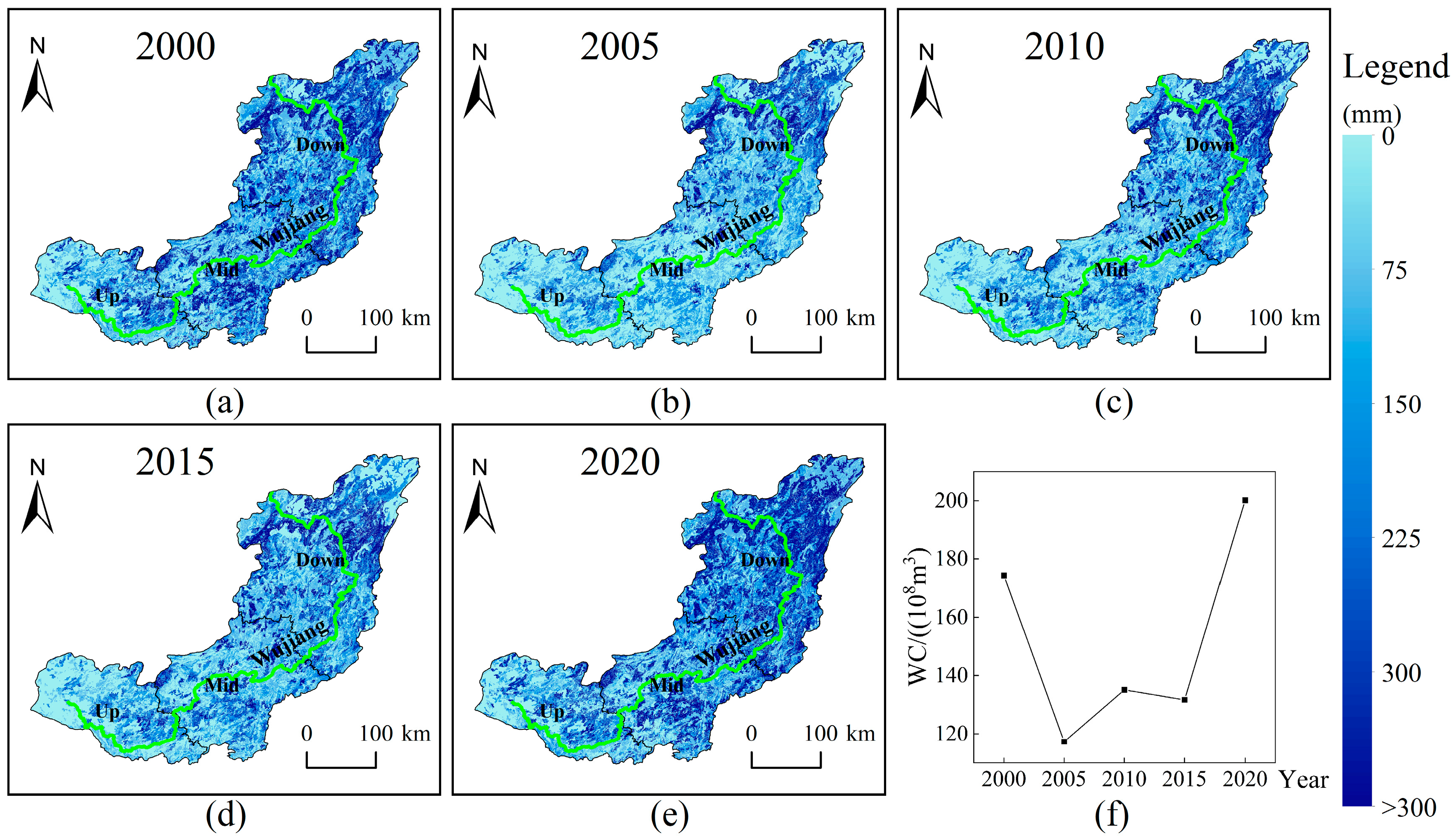
- Water conservation
- 5.
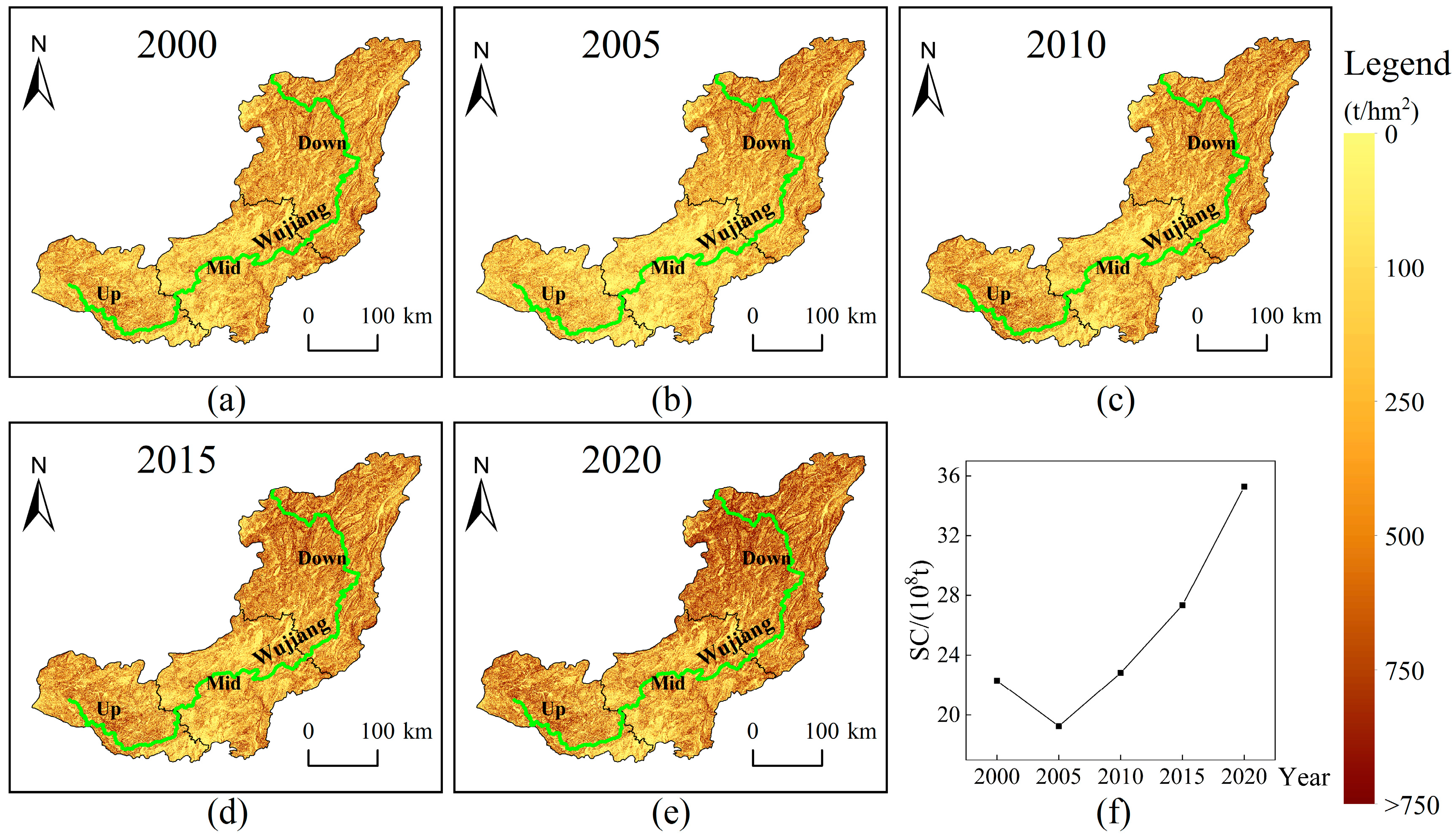
- Soil conservation
- 6.
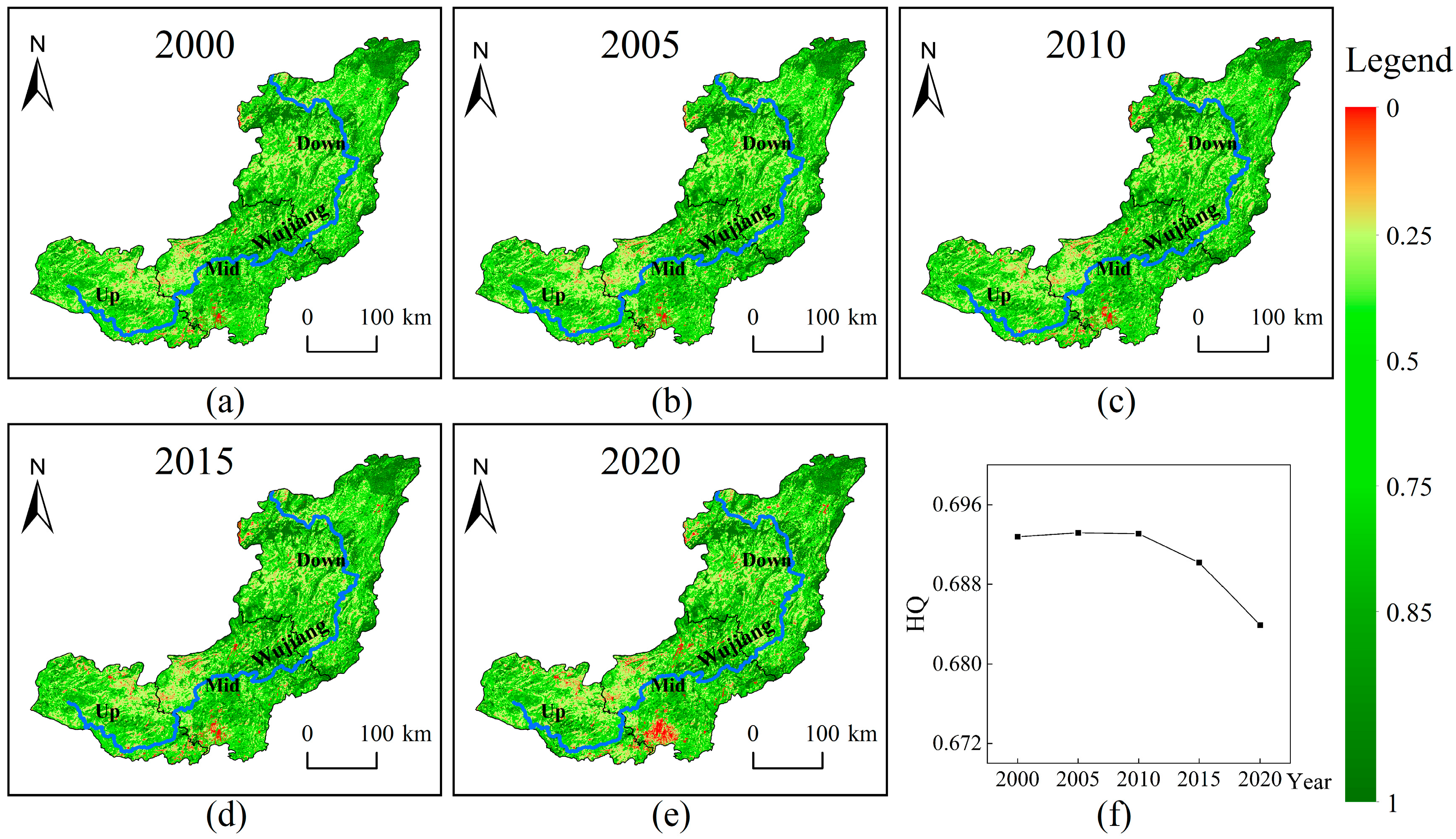
- Habitat quality
2.3.2. Trends in ESs in the Time Dimension
2.3.3. Trade-Offs and Synergy Analysis of ESs
2.3.4. ESB Analysis
2.3.5. Nonlinear Relationship of ESs
3. Results
3.1. ES Assessment Results
3.2. Spatiotemporal Trends in ESs
3.3. Trade-Offs and Synergy Analysis of ESs
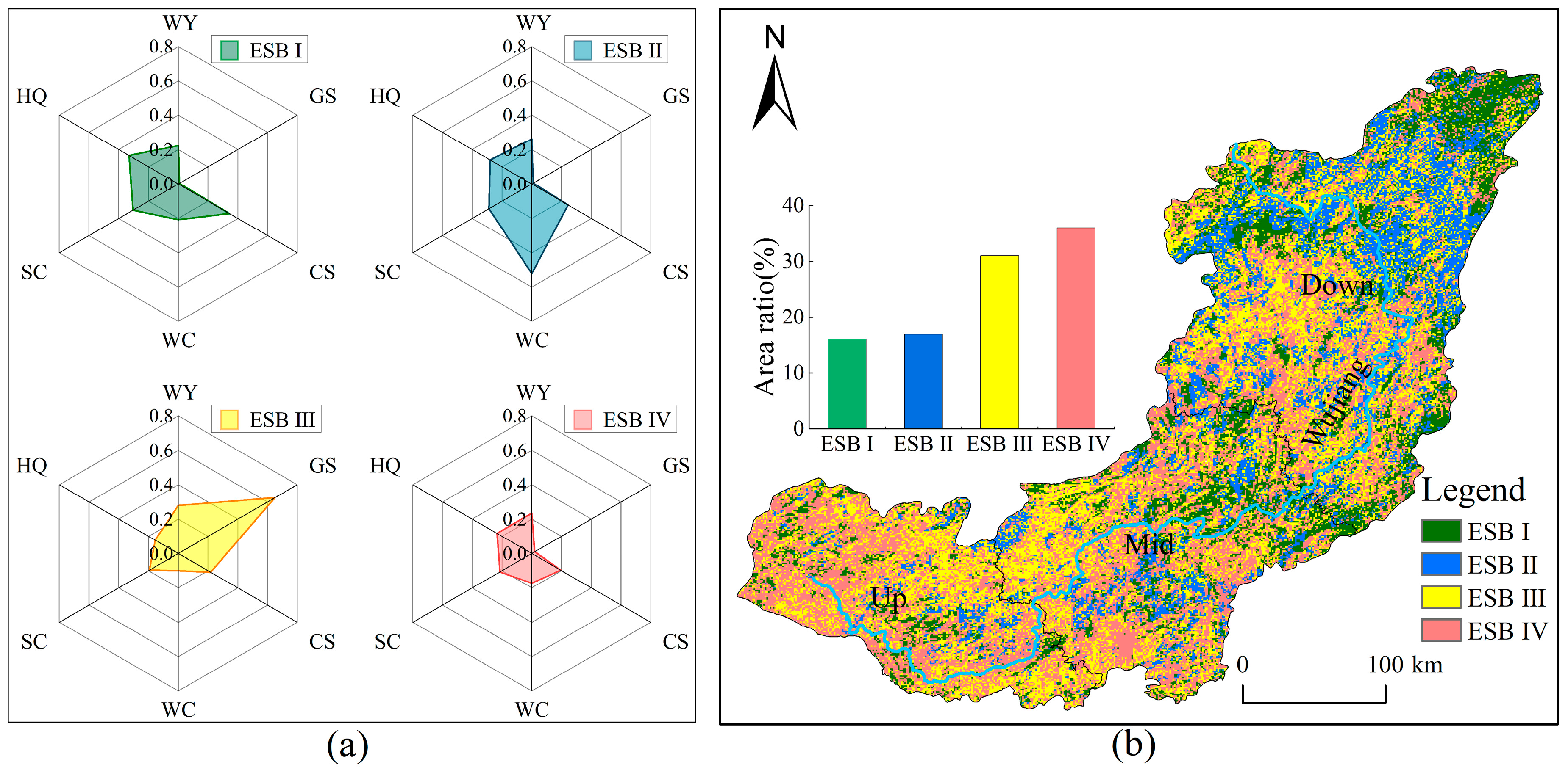
3.4. Compositional Structure and Spatial Pattern of ESBs
3.5. Nonlinear Relationship of ESs
4. Discussion
4.1. ES Spatial–Temporal Characteristics
4.2. ES Trade-Offs/Synergies
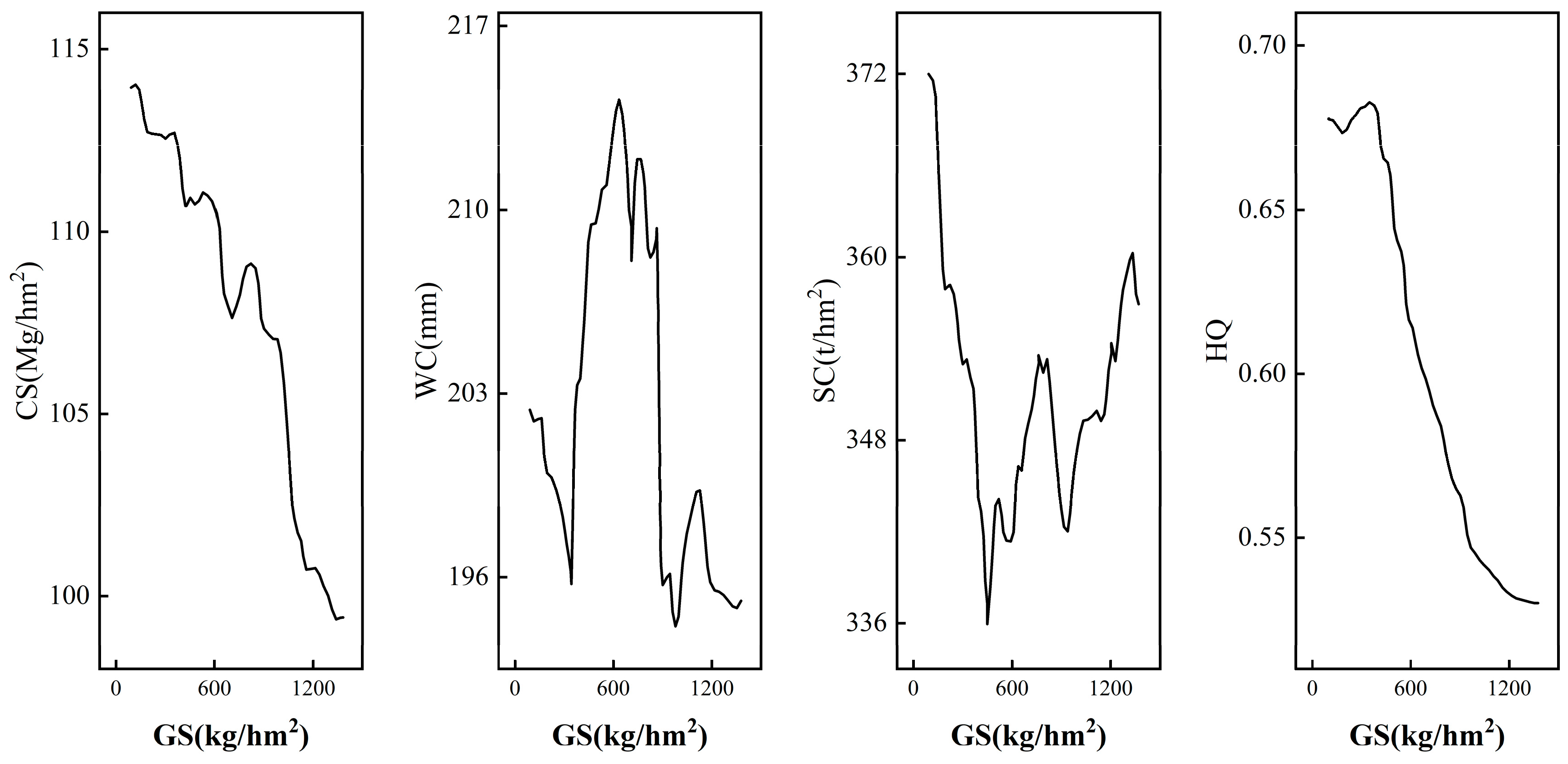
4.3. Nonlinear Relationship of ESs
5. Conclusions
- (1)
- In general, ESs in the WJRB spatially show the order downstream > midstream > upstream. They show the largest increase upstream and the largest decrease midstream in the time dimension.
- (2)
- WS, WC, and SC in the WJRB underwent a trend shift in 2005, mainly owing to climatic influences, whereas GS and HQ underwent a trend shift in 2010, mainly owing to human social development.
- (3)
- In the spatial pattern, GS formed a trade-off with other ESs; in the temporal dimension, WS formed a trade-off with other ESs owing to the influence of karst geology on the WJRB.
- (4)
- Implementing major ecological projects and increasing grain production per unit area are effective ways to reduce the spatial trade-off between ESs. Focusing on monitoring erosion-prone areas to prevent widespread soil erosion during heavy precipitation years is a strategy to reduce the temporal trade-off between ESs in karst areas such as the WJRB.
Author Contributions
Funding
Data Availability Statement
Conflicts of Interest
References
- Carpenter, S.R.; Mooney, H.A.; Agard, J.; Capistrano, D.; DeFries, R.S.; Diaz, S.; Dietz, T.; Duraiappah, A.K.; Oteng-Yeboah, A.; Pereira, H.M.; et al. Science for managing ecosystem services: Beyond the Millennium Ecosystem Assessment. Proc. Natl. Acad. Sci. USA 2009, 106, 1305–1312. [Google Scholar] [CrossRef] [PubMed]
- Cord, A.; Bartkowski, B.; Beckmann, M.; Dittrich, A.; Hermans, K.; Kaim, A.; Lienhoop, N.; Locher, K.; Priess, J.; Schröter-Schlaack, C.; et al. Towards systematic analyses of ecosystem service trade-offs and synergies: Main concepts, methods and the road ahead. Ecosyst. Serv. 2017, 28, 264–272. [Google Scholar] [CrossRef]
- Li, S.C.; Zhang, C.Y.; Liu, J.L.; Zhum, W.B.; Ma, C.; Wang, Y. Research progress on ecosystem service trade-off and synergy and research topics in geography. Geogr. Res. 2013, 32, 1379–1390. (In Chinese) [Google Scholar]
- Liu, G.B.; Shao, Q.N.; Fan, J.W.; Ning, J.; Huang, H.B.; Liu, S.C.; Zhang, X.Y.; Niu, L.N.; Liu, J.Y. Spatio-Temporal Changes, Trade-Offs and Synergies of Major Ecosystem Services in the Three-River Headwaters Region from 2000 to 2019. Remote Sens. 2022, 14, 5349. [Google Scholar] [CrossRef]
- Zheng, D.; Wang, Y.; Hao, S.; Xu, W.; Lv, L.; Yu, S. Spatial-temporal variation and tradeoffs/synergies analysis on multiple ecosystem services: A case study in the Three-River Headwaters region of China. Ecol. Indic. 2020, 116, 106494. [Google Scholar] [CrossRef]
- Chen, T.; Feng, Z.; Zhao, H.; Wu, K. Identification of ecosystem service bundles and driving factors in Beijing and its surrounding areas. Sci. Total Environ. 2020, 711, 134687. [Google Scholar] [CrossRef]
- Lu, N.; Fu, B.; Jin, T.; Chang, R. Trade-off analyses of multiple ecosystem services by plantations along a precipitation gradient across Loess Plateau landscapes. Landsc. Ecol. 2014, 29, 1697–1708. [Google Scholar] [CrossRef]
- Li, T.; Liang, S.Y.; Zhang, J.; Geng, Y.; Geng, T.W.; Shi, J.X. A Bayesian network-based analysis of ecosystem service trade-off synergies and their drivers on the Loess Plateau of northern Shaanxi. Acta Ecol. Sin. 2023, 43. (In Chinese) [Google Scholar] [CrossRef]
- Wang, L.N.; Yu, E.Y.; Li, S.; Fu, X.; Wu, G. Analysis of Ecosystem Service Trade-Offs and Synergies in Ulansuhai Basin. Sustainability 2021, 13, 9839. [Google Scholar] [CrossRef]
- Luo, Y.Y.; Yang, D.W.; O’Connor, P.; Wu, T.H.; Ma, W.J.; Xu, L.X.; Guo, R.F.; Lin, J.Y. Dynamic characteristics and synergistic effects of ecosystem services under climate change scenarios on the Qinghai-Tibet Plateau. Sci. Rep. 2022, 12, 2540. [Google Scholar] [CrossRef]
- Zhang, B.W.; Zheng, L.; Wang, Y.; Li, N.; Li, J.F.; Yang, H.; Bi, Y.Z. Multiscale ecosystem service synergies/trade-offs and their driving mechanisms in the Han River Basin, China: Implications for watershed management. Environ. Sci. Pollut. Res. 2023, 30, 43440–43454. [Google Scholar] [CrossRef] [PubMed]
- Han, H.Q.; Yin, C.Y.; Zhang, C.Q.; Gao, H.J.; Bai, Y.M. Response of trade-offs and synergies between ecosystem services and land use change in the Karst area. Trop. Ecol. 2019, 60, 230–237. [Google Scholar] [CrossRef]
- Zhou, S.Y.; Li, W.; Lu, Z.Y.F.; Cheng, R.H. An ecosystem-based analysis of urban sustainability by integrating ecosystem service bundles and socio-economic-environmental conditions in China. Ecol. Indic. 2020, 117, 106691. [Google Scholar] [CrossRef]
- Shen, J.; Li, S.; Liang, Z.; Liu, L.; Li, D.; Wu, S. Exploring the heterogeneity and nonlinearity of trade-offs and synergies among ecosystem services bundles in the Beijing-Tianjin-Hebei urban agglomeration. Ecosyst. Serv. 2020, 43, 101103. [Google Scholar] [CrossRef]
- Gou, M.; Li, L.; Ouyang, S.; Wang, N.; La, L.M.; Liu, C.F.; Xiao, W.F. Identifying and analyzing ecosystem service bundles and their socioecological drivers in the Three Gorges Reservoir Area. J. Clean. Prod. 2021, 307, 127208. [Google Scholar] [CrossRef]
- Yang, J.Y.; Li, J.S.; Guan, X. Spatial and temporal patterns and driving mechanisms of carbon sequestration services in the Wujiang River Basin. Environ. Sci. Res. 2023, 36, 757–767. (In Chinese) [Google Scholar]
- Qiu, S.J.; Peng, J.; Zheng, H.N.; Xu, Z.H.; Meersmans, J. How can massive ecological restoration programs interplay with social-ecological systems? A review of research in the South China karst region. Sci. Total Environ. 2022, 807, 150723. [Google Scholar] [CrossRef]
- Huang, Q.; Peng, L.; Huang, K.X.; Deng, W.; Liu, Y. Generalized Additive Model Reveals Nonlinear Trade-Offs/Synergies between Relationships of Ecosystem Services for Mountainous Areas of Southwest China. Remote Sens. 2022, 14, 2733. [Google Scholar] [CrossRef]
- Yao, F.M.; Tang, Y.J.; Wang, P.J.; Zhang, J.H. Estimation of maize yield by using a process-based model and remote sensing data in the Northeast China Plain. Phys. Chem. Earth Parts A/B/C 2015, 87–88, 142–152. [Google Scholar] [CrossRef]
- Zhang, Y.; Gurung, R.; Marx, E.; Williams, S.; Ogle, S.; Paustian, K. DayCent Model Predictions of NPP and Grain Yields for Agricultural Lands in the Contiguous, U.S. J. Geophys. Res. Biogeosci. 2020, 125, e2020JG005750. [Google Scholar] [CrossRef]
- Abera, W.; Tamene, L.; Kassawmar, T.; Mulatu, K.; Kassa, H.; Verchot, L.; Quintero, M. Impacts of land use and land cover dynamics on ecosystem services in the Yayo coffee forest biosphere reserve, southwestern Ethiopia. Ecosyst. Serv. 2021, 50, 101338. [Google Scholar] [CrossRef]
- Xia, L.; An, Y.L.; Jiang, H.F.; Wu, X.; Hao, X.C. InVEST modeling-based water conservation in karst watersheds—A case study of Wujiang River Basin in Guizhou Province. Guizhou Sci. 2019, 37, 27–32. (In Chinese) [Google Scholar]
- Liu, Y.; Zhou, Y.; Du, Y.T. Characteristics of spatial and temporal differentiation of habitat quality in the middle reaches of the Yangtze River economic zone and its topographic gradient effect based on the InVEST model. Yangtze River Basin Resour. Environ. 2019, 28, 2429–2440. (In Chinese) [Google Scholar]
- Wu, J.S.; Li, X.C.; Luo, Y.H.; Zhang, D.N. Spatiotemporal effects of urban sprawl on habitat quality in the Pearl River Delta from 1990 to 2018. Sci. Rep. 2021, 11, 13981. [Google Scholar] [CrossRef] [PubMed]
- Wang, C.J.; Zhao, H.R. Analysis of remote sensing time-series data to foster ecosystem sustainability: Use of temporal information entropy. Int. J. Remote Sens. 2019, 40, 2880–2894. [Google Scholar] [CrossRef]
- Wang, C.J. Temporal Information Entropy and Its Application in the Evaluation of Ecological Environment Quality in the Yanhe River Basin; Tsinghua University: Beijing, China, 2016. (In Chinese) [Google Scholar]
- Feng, Z.; Peng, J.; Wu, J.S. Spatial and temporal evolution of ecosystem services in Shenzhen based on ecosystem service clusters. Acta Ecol. Sin. 2020, 40, 2545–2554. [Google Scholar]
- Friedman, J.H. Greedy function approximation: A gradient boosting machine. Ann. Stat. 2001, 29, 1189–1232. [Google Scholar] [CrossRef]
- Amundson, R.; Berhe, A.; Hopmans, J. Soil and human security in the 21st century. Science 2015, 48, 1261071. [Google Scholar] [CrossRef]
- Di, Y.P.; Zhang, Y.J.; Zeng, F.; Tang, Z. Impacts of changes in the “Asian Water Tower” on the Qinghai-Tibet Plateau ecosystem. Bull. Chin. Acad. Sci. 2019, 34, 1322–1331. (In Chinese) [Google Scholar]
- Niu, Z.E.; He, H.L.; Ren, S.L.; Zhang, L.; Qin, K.Y.; Zhao, D.; Lv, Y. Spatial and temporal dynamics of terrestrial ecosystem services and their trade-offs and synergies in China from 2000–2018 based on process model. J. Ecol. 2023, 43, 496–509. (In Chinese) [Google Scholar]
- Piao, S.L.; He, Y.; Wang, X.H.; Chen, F.H. Estimation of China’s terrestrial ecosystem carbon sink: Methods, progress and prospects. Sci. China-Earth Sci. 2022, 65, 641–651. [Google Scholar] [CrossRef]
- Tang, X.L.; Zhao, X.; Bai, Y.F.; Tang, Z.Y.; Wang, W.T.; Zhao, Y.C.; Wan, H.W.; Xie, Z.Q.; Shi, X.Z.; Wu, B.F.; et al. Carbon pools in China’s terrestrial ecosystems: New estimates based on an intensive field survey. Proc. Natl. Acad. Sci. USA 2018, 115, 4021–4026. [Google Scholar] [CrossRef] [PubMed]
- Wu, X.; Shi, W.; Tao, F. Estimations of forest water retention across China from an observation site-scale to a national-scale. Ecol. Indic. 2021, 132, 108274. [Google Scholar] [CrossRef]
- Yu, G.R.; Yang, M.; Chen, Z.; Zhang, L.M. Technical approaches and strategic layout of large-scale regional ecological environment management and national ecological security pattern construction. J. Appl. Ecol. 2021, 32, 1141–1153. (In Chinese) [Google Scholar]
- Zhao, M.; Di, D.R.; Huang, G.W.; Shi, W.Y. Spatial pattern evolution and coupling characteristics of economy and population in Wujiang River Basin. Soil Water Conserv. Res. 2022, 29, 298–310+21. (In Chinese) [Google Scholar]
- Guo, W.X.; Hu, J.W.; Wang, H.X. Analysis of Runoff Variation Characteristics and Influencing Factors in the Wujiang River Basin in the Past 30 Years. Int. J. Environ. Res. Public Health 2022, 19, 372. [Google Scholar] [CrossRef]
- Yu, Y.H.; Sun, X.Q.; Wang, J.L.; Zhang, J.P. Using InVEST to evaluate water yield services in Shangri-La, Northwestern Yunnan, China. PeerJ 2022, 10, e12804. [Google Scholar] [CrossRef]
- Wang, J.; Zhao, W.W.; Liu, Y.; Jia, L.Z. A review of research on the effects of plant functional traits on soil conservation. Acta Ecol. Sin. 2019, 39, 3355–3564. (In Chinese) [Google Scholar]
- Liu, Y.S.S.; Yang, R.; Lin, Y.C. Evolution and optimization of county urbanization patterns in China. Acta Geogr. Sin. 2022, 77, 2937–2953. (In Chinese) [Google Scholar]
- Albert, J.S.; Carnaval, A.C.; Flantua, S.G.A.; Lohmann, L.G.; Ribas, C.C.; Riff, D.; Carrillo, J.D.; Fan, Y.; Figueiredo, J.J.P.; Guayasamin, J.M.; et al. Human impacts outpace natural processes in the Amazon. Science 2023, 379, eabo5003. [Google Scholar] [CrossRef]
- Yang, J.; Xie, B.; Zhang, D. The Trade-Offs and Synergistic Relationships between Grassland Ecosystem Functions in the Yellow River Basin. Diversity 2021, 13, 505. [Google Scholar] [CrossRef]
- Shao, Q.Q.; Liu, S.C.; Ning, J.; Liu, G.B.; Yang, F.; Zhang, X.Y.; Niu, L.N.; Huang, H.B.; Fan, J.W.; Liu, J.Y. Remote sensing assessment of ecological benefits of major ecological projects in China from 2000–2019. Acta Geogr. Sin. 2022, 77, 2133–2153. (In Chinese) [Google Scholar]
- Dai, E.F.; Wang, X.L.; Zhu, J.J.; Zhao, D.S. Ecosystem service trade-offs: Methods, models, and research frameworks. Geogr. Res. 2016, 35, 1005–1016. (In Chinese) [Google Scholar]
- Liu, S.J.; Wang, Z.J.; Wu, W.; Yu, L. Effects of landscape pattern change on ecosystem services and its interactions in karst cities: A case study of Guiyang City in China. Ecol. Indic. 2022, 145, 109646. [Google Scholar] [CrossRef]
- Bennett, E.; Peterson, G.; Gordon, L. Understanding relationships among ecosystem services. Ecol Lett. 2009, 12, 1394–1404. [Google Scholar] [CrossRef]
- Jha, S.; Egerer, M.; Bichier, P.; Cohen, H.; Liere, H.; Lin, B.; Lucatero, A.; Philpott, S. Multiple ecosystem service synergies and landscape mediation of biodiversity within urban agroecosystems. Ecol. Lett. 2023, 26, 369–383. [Google Scholar] [CrossRef]
- Power, A.G. Ecosystem services and agriculture: Tradeoffs and synergies. Philos. Trans. R. Soc. London. Ser. B Biol. Sci. 2010, 365, 2959–2971. [Google Scholar] [CrossRef]
- Jing, H.C.; Liu, Y.H.; He, P.; Zhang, J.Q.; Dong, J.Y.; Wang, Y. Spatial heterogeneity of ecosystem services and its influencing factors in typical areas of the Tibetan Plateau: The case of Nagqu City. Acta Ecol. Sin. 2022, 42, 2657–2673. (In Chinese) [Google Scholar]
- Fu, G. A Study on the Trade-Offs and Synergistic Relationships between Landscape Pattern Evolution and Ecosystem Services in China’s Land Areas over the Past 40 Years; Beijing Normal University: Beijing, China, 2022. (In Chinese) [Google Scholar]
- Dong, B.G.; Yu, Y.; Pereira, P. Non-growing season drought legacy effects on vegetation growth in southwestern China. Sci. Total Environ. 2022, 846, 157334. [Google Scholar] [CrossRef]
- Xiao, L.G.; Li, G.Q.; Zhao, R.Q.; Zhang, L. Effects of soil conservation measures on wind erosion control in China: A synthesis. Sci. Total Environ. 2021, 778, 146308. [Google Scholar] [CrossRef]
- Cai, D.W.; Ge, Q.S.; Wang, X.M.; Liu, B.L.; Andrew, S.G.; Hu, S. Contributions of ecological programs to vegetation restoration in arid and semiarid China. Environ. Res. Lett. 2020, 15, 114046. [Google Scholar] [CrossRef]
- Guo, Q.K.; Zhong, R.H.; Shan, Z.J.; Duan, X. Vegetation Cover Variation in Dry Valleys of Southwest China: The Role of Precipitation. Remote Sens. 2023, 15, 1727. [Google Scholar] [CrossRef]
- Liu, J.Z.; Yang, L.; Jiang, J.C.; Yuan, W.; Duan, Z. Mapping diurnal cycles of precipitation over China through clustering. J. Hydrol. 2021, 592, 125804. [Google Scholar] [CrossRef]
- Yang, J.Y.; Guan, X.; Li, J.S.; Liu, J.; Hao, H.; Wang, H. Spatial patterns and interrelationships of biodiversity and ecosystem services in the Wujiang River Basin. Biodivers. Sci. 2023, 31, 23061. [Google Scholar] [CrossRef]
- Fang, J.; Piao, S.; Zhou, L.; He, J.; Wei, F.; Myneni, R.B.; Tucker, C.J.; Tan, K. Precipitation patterns alter growth of temperate vegetation. Geophys. Res. Lett. 2005, 32. [Google Scholar] [CrossRef]
- Xu, X.J.; Yan, Y.J.; Dai, Q.H.; Yi, X.S.; Hu, Z.Y.; Cen, L.P. Spatial and temporal dynamics of rainfall erosivity in the karst region of southwest China: Interannual and seasonal changes. Catena 2023, 221, 106763. [Google Scholar] [CrossRef]
- Li, Z.W.; Xu, X.L.; Zhu, J.X.; Zhong, F.X.; Xu, C.H.; Wang, K.L. Can precipitation extremes explain variability in runoff and sediment yield across heterogeneous karst watersheds? J. Hydrol. 2021, 596, 125698. [Google Scholar] [CrossRef]
- Yue, X.L.; Wu, S.H.; Huang, M.; Gao, J.B.; Yin, Y.H.; Feng, A.Q.; Gu, X.P. Spatial association between landslides and environmental factors over Guizhou Karst Plateau, China. J. Mt. Sci. 2018, 15, 1987–2000. [Google Scholar] [CrossRef]
- Grasso, M. Ecological–economic model for optimal mangrove trade off between forestry and fishery production: Comparing a dynamic optimization and a simulation model. Ecol. Model. 1998, 112, 131–150. [Google Scholar] [CrossRef]
- Spake, R.; Lasseur, R.; Crouzat, E.; Bullock, J.M.; Lavorel, S.; Parks, K.E.; Schaafsma, M.; Bennett, E.M.; Maes, J.; Mulligan, M.; et al. Unpacking ecosystem service bundles: Towards predictive mapping of synergies and trade-offs between ecosystem services. Glob. Environ. Chang. 2017, 47, 37–50. [Google Scholar] [CrossRef]


| Date Type | Date Name | Data Sources |
|---|---|---|
| Land-use data | Land use | Derived from Earth System Science Data (earth-system-science-data.net, accessed on 1 March 2023) at a spatial resolution of 30 m. |
| Meteorological data | Average annual potential evapotranspiration | Derived from the National Earth System Science Data Center (http://loess.geodata.cn, accessed on 1 March 2023), with a spatial resolution of 1 km. |
| Average monthly precipitation | ||
| Average annual precipitation | ||
| Soil data | Soil depth | Derived from the National Tibetan Plateau Science Data Center (data.tpdc.ac.cn/, accessed on 1 March 2023) at a spatial resolution of 1 km. |
| Soil texture (sand, clay, powder) content | ||
| Soil organic matter content | ||
| Soil capacity | ||
| Natural surface factor | Normalized Difference Vegetation Index (NDVI) | Derived from MODIS Vegetation Index product data MOD13Q1 (https://earthdata.nasa.gov, accessed on 1 March 2023) at 250 m spatial resolution. |
| Altitude | Derived from Geospatial Data Cloud (http://www.gscloud.cn, accessed on 1 March 2023), spatial resolution 30 m. | |
| Slope | Calculated based on elevation data with a spatial resolution of 30 m. | |
| Aspect | ||
| Net ecosystem productivity (NEP) | Derived from the National Earth System Science Data Center (http://loess.geodata.cn, accessed on 1 March 2023), with a spatial resolution of 500 m. | |
| Net primary productivity (NPP) | Derived from MODIS vegetation index product data (https://earthdata.nasa.gov, accessed on 1 March 2023) at 500 m spatial resolution. | |
| Carbon density data | Carbon densities of aboveground biomass, belowground biomass, soil, and apoplankton | Derived from Chinese scientific data (http://csdata.org/, accessed on 1 March 2023). |
Disclaimer/Publisher’s Note: The statements, opinions and data contained in all publications are solely those of the individual author(s) and contributor(s) and not of MDPI and/or the editor(s). MDPI and/or the editor(s) disclaim responsibility for any injury to people or property resulting from any ideas, methods, instructions or products referred to in the content. |
© 2023 by the authors. Licensee MDPI, Basel, Switzerland. This article is an open access article distributed under the terms and conditions of the Creative Commons Attribution (CC BY) license (https://creativecommons.org/licenses/by/4.0/).
Share and Cite
Yang, J.; Li, J.; Fu, G.; Liu, B.; Pan, L.; Hao, H.; Guan, X. Spatial and Temporal Patterns of Ecosystem Services and Trade-Offs/Synergies in Wujiang River Basin, China. Remote Sens. 2023, 15, 4099. https://doi.org/10.3390/rs15164099
Yang J, Li J, Fu G, Liu B, Pan L, Hao H, Guan X. Spatial and Temporal Patterns of Ecosystem Services and Trade-Offs/Synergies in Wujiang River Basin, China. Remote Sensing. 2023; 15(16):4099. https://doi.org/10.3390/rs15164099
Chicago/Turabian StyleYang, Junyi, Junsheng Li, Gang Fu, Bo Liu, Libo Pan, Haojing Hao, and Xiao Guan. 2023. "Spatial and Temporal Patterns of Ecosystem Services and Trade-Offs/Synergies in Wujiang River Basin, China" Remote Sensing 15, no. 16: 4099. https://doi.org/10.3390/rs15164099
APA StyleYang, J., Li, J., Fu, G., Liu, B., Pan, L., Hao, H., & Guan, X. (2023). Spatial and Temporal Patterns of Ecosystem Services and Trade-Offs/Synergies in Wujiang River Basin, China. Remote Sensing, 15(16), 4099. https://doi.org/10.3390/rs15164099