1. Introduction
Change detection (CD), in remote sensing images, refers to the process of observing, analyzing, and identifying differences in ground objects at different times [
1]. This process enables efficient and dynamic monitoring of ground objects and has significant applications in urban planning, disaster monitoring, resource management, and other fields [
2].
Change detection can be classified into binary change detection (BCD) and semantic change detection (SCD) based on their detection purposes. While BCD has been extensively studied and utilized, it falls short in providing a comprehensive understanding and analysis of the phenomenon by solely identifying the location of the change. SCD addresses this limitation by considering the land cover categories associated with the changed areas [
3,
4]. By analyzing the specific land cover categories affected by the changes, researchers can gain a more comprehensive understanding of the change process, enabling them to delve into the reasons and impacts of the detected changes. This comprehensive understanding is crucial for various applications, including urbanization studies, environmental monitoring, resource surveys, and related research. These fields typically require not only knowledge of the location of changes but also a deeper understanding of the types and characteristics of the changes. SCD aims to bridge this gap and enhance the quality and interpretability of the change detection results [
5,
6,
7].
In recent years, with the improvement of remote sensing image (RSI) quality, high-resolution images have gradually become the primary data source for CD tasks. However, high-resolution images typically contain abundant texture information, as well as variations in non-structured lighting conditions and complex backgrounds. Consequently, traditional change detection methods relying on handcrafted designed features struggle to fully capture the nuanced change information, leading to poor robustness [
8,
9]. In contrast, remote sensing image processing and analysis methods based on deep learning offers several advantages over traditional methods, including strong applicability and high accuracy. Deep learning techniques are capable of extracting non-linear features and have flexible network structures, greatly enhancing their performance in various remote sensing applications, such as dynamic object tracking [
10], fruit detection [
11], oil spill monitoring [
12], among others. Furthermore, their development potential far exceeds that of traditional methods [
13].
Deep learning-based approaches in SCD have achieved good performance, including independent three-branch networks (which respectively handle semantic segmentation (SS) and BCD) [
14], post-classification change detection methods [
15], and direct classification methods, etc. However, these methods commonly ignore the inherent relationship between the two sub-tasks and encounter challenges in effectively acquiring temporal features, which limits the precision of SCD. To address these challenges, multi-task SCD methods utilizing Siamese networks have emerged, extracting dual-temporal image features and feeding them into separate task branches, resulting in improved accuracy [
16,
17]. Nonetheless, these methods have certain limitations, particularly in their ability to capture detailed features, which can lead to the missed or false detection of small targets and inaccurate boundaries. Another important aspect that requires further investigation is the imbalanced problem between the SS and BCD tasks during training. This imbalance can impact the recognition of LC categories and ultimately limit the performance of the SS subtask. Therefore, addressing these issues is crucial for improving the overall effectiveness and accuracy of these detection methods.
To fully utilize spatial details and adaptively balance the performance of the two sub-tasks, this paper proposed a spatial-temporal semantic perception network (STSP-Net) for high-resolution remote sensing SCD. This STSP-Net simultaneously captures spatial details and contextual information through detail-aware and contextual paths. Moreover, it incorporates two designed modules for adaptive learning, which fuse spatial details and deep semantic features, enhance foreground semantic features, reduce pseudo-changes, and ultimately improve the accuracy of SCD.
The main contributions of this paper were as follows:
We proposed a novel STSP-Net to improve SCD performance in high-resolution RSIs. Through the implementation of the detail-aware path (DAP) to extract shallow detailed features and adaptively aligning the deep contextual information, we fused the two types of features to enhance spatial-temporal semantic perception;
We designed a spatial attention fusion module (SAFM) and a temporal refinement detection module (TRDM) in the STSP-Net to strengthen spatial semantic learning, increase the sensitivity of temporal features to the changing areas, and balance the performance of the SS and BCD subtasks;
We developed a concise invariant consistency loss function (ICLoss) based on the metric learning strategy to constrain the consistency of land cover in the unchanged areas, which highlighted the changing areas.
The driving motivation behind this research was to contribute to the current understanding of SCD, rectifying the deficiencies observed in existing methodologies pertaining to spatial detail extraction, task imbalance, and consistency enforcement. By expanding the boundaries of research in the realm of remote sensing, our study provides a more accurate and interpretable approach to semantic change detection, thus bridging the gap between theoretical advancements and practical applications.
The rest of this paper is organized as follows.
Section 2 reviews related work.
Section 3 provides a detailed description of the proposed method.
Section 4 describes the dataset and experimental setup.
Section 5 presents the experimental results and discusses them. Finally,
Section 6 summarizes the work of this paper.
2. Related Work
In this section, we will first review the current research status of BCD, which serves as the foundation for the task of SCD. BCD has undergone extensive research and development, providing valuable insights into the location of changes. Building upon this foundation, SCD goes a step further by identifying LC categories to provide additional information. Therefore, after discussing the current research status of BCD, we will delve into a detailed exploration of the research related to SCD.
2.1. Binary Change Detection
With the continuous progress of computer technology and the rapid popularization of RSI technology in recent years, BCD has gradually become an important research area in RSI analysis. Traditional BCD algorithms can usually be categorized into visual analysis, algebra-based methods [
18,
19], transform-based methods [
20,
21], classification methods, advanced models, and other hybrid approaches. However, due to the limitations of handcrafted feature extraction and complex threshold adjustment, traditional methods face challenges in adapting to different data and change patterns, and their application scope is limited [
22].
Compared with traditional methods, deep learning methods exhibit powerful feature learning capabilities and flexible model structures, which greatly improve the performance of BCD [
13]. Deep learning-based BCD networks are commonly classified into two types: single-stream and double-stream networks.
Single-stream networks are based on semantic segmentation networks and employ different methods to fuse two or multiple-phase RSIs as inputs. Direct concatenation [
23], difference images [
24], or change analysis methods [
25] are commonly used data fusion methods. Direct concatenation can preserve all information from multi-temporal RSIs. Change analysis, difference images, and other methods can provide or highlight change information in dual-temporal RSIs to facilitate CD.
Double-stream networks typically consist of two feature extraction streams with shared weights, which can leverage the correlation between the bi-temporal image datasets for training and learning more accurate feature representations [
26]. Therefore, most researchers currently use the Siamese network structure for change detection [
27].
To overcome the various challenges in BCD and improve the accuracy and applicability of deep learning methods, researchers have conducted extensive studies and have proposed numerous methods. For instance, there is the SRCDNet [
28], which is suitable for different resolution images. The GAS-Net [
29] overcomes the class imbalance problem. The DTCDSCN [
30] and the SFCCD network [
31] alleviate the issues of incomplete regions and irregular boundaries. The DASNet [
32] and the SDACD network [
33] can resist pseudo-changes. Additionally, there are also networks that have been designed specifically for building change detection, such as the LGPNet [
34], MDEFNET [
35], and HDANet [
36]. Overall, researchers have made significant progress in improving the accuracy and applicability of RSI change detection by introducing new network structures and algorithms to address the challenges of BCD.
Although existing BCD methods can locate the occurrence of changes and the problems of pseudo-changes, small-target change detection, and change region boundary recognition are gradually improving, these methods cannot provide information on the types of changes, which cannot meet the demand for change-type information in practical applications. Therefore, it is necessary to further enhance change detection methods in order to accurately identify multiple types of changes and provide richer information to support a wider range of applications.
2.2. Semantic Change Detection
SCD plays a crucial role in simultaneously identifying the changed areas and the LC categories in bi-temporal RSIs. It has wide-ranging applications across various fields, such as new photovoltaic detection, non-agricultural land conversion, and urban planning. Early methods for SCD included intuitive techniques, like post-classification comparison [
37], direct classification [
38,
39], and other methods. With the development of deep learning, more attention has been paid to the research of SCD [
4]. As previously analyzed in the literature [
5,
16], existing deep learning frameworks for SCD can be mainly categorized into three types: (1) frameworks based on SS networks; (2) frameworks based on CD networks; and (3) frameworks based on multi-task learning.
Frameworks based on SS can be further divided into two types: (1) the post-classification change detection (PCCD) method, as shown in
Figure 1a, which judges the existence of change areas by comparing the SS results of dual-temporal images. For example, Xia et al. [
15] proposed a deep Siamese fusion post-classification network, and Peng et al. [
40] proposed a SCD method based on the Siamese U-Net network, which further introduced metric learning and deep supervision strategies to improve the network performance. The drawbacks of this method are that its accuracy mainly depends on the accuracy of the predicted land cover map, and that the prediction error will accumulate gradually. (2) The fused-prior segmentation method (FPSM), as shown in
Figure 1b, which inputs the fused two-period images into the SS network, with each label representing a type of change. This method includes several methods that treat CD as a SS task, such as FC-EF [
27].
Frameworks based on CD networks mainly refers to the single-output branch Siamese network (SOBSN), as shown in
Figure 1c, which extracts image pair features through a shared-weight encoder and inputs them into a decoder for multi-class change detectionnetworks, such as FC-Siam-conc, FC-Siam-diff [
27], ReCNN [
41], and others, belong to this category. This method shares the same limitation as FPSM, which is the quadratic increase in the number of change categories with the number of land cover categories considered. Moreover, in combination with the issue of class imbalance, training becomes more challenging.
Frameworks based on multi-task learning comprise two main types of architectures: (1) the independent semantic segmentation and change detection network (ISSCDN). As shown in
Figure 1d, this network simultaneously trains completely separate branches for BCD and SS, completely ignoring the temporal correlation between the two temporal images and the inherent correlation between the two sub-tasks. The representative architecture of this type is HRSCD-sr.3 [
5]. (2) The multi-output branch Siamese network (MOBSN). As shown in
Figure 1e, both sub-tasks adopt a Siamese network for feature extraction and then use different prediction branches to complete their tasks, alleviating the previous method’s drawback of ignoring the temporal correlation. This architecture is represented by the SSCD-l structure by the authors of [
16]. The discussions made by the authors of [
5,
16] unanimously agree that the MOBSN architecture achieves the best overall results. These works demonstrate the potential for mutual promotion between the BCD and SS tasks [
30,
31], and also reveal the feasibility of multi-task deep learning in the SCD tasks. For example, Zheng et al. [
17] proposed a multi-task architecture called ChangeMask, which decouples SCD into temporal SS and BCD, and designs a time-symmetric Transformer module to ensure temporal symmetry. Chen et al. [
42] proposed a feature-constrained change detection network, which demonstrated that dual-temporal SS branches can improve the accuracy of BCD tasks.
Despite the existence of research on SCD for a considerable period, it is still in its nascent stages and necessitates thorough exploration and experimentation using algorithmic processes, model structures, and dataset construction [
4]. The multi-task SCD method based on Siamese networks has been used in some studies and has achieved certain results. Nonetheless, this approach encounters certain challenges, including limited sensitivity to details and task imbalance when dealing with class-imbalanced data, leading to inadequate accuracy and robustness. Therefore, this paper proposed a STSP-Net, which aims to tackle these challenges.
3. Method
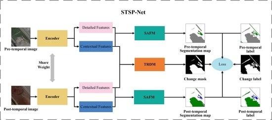
In this section, we provide a detailed introduction to the proposed spatial-temporal semantic perception network (STSP-Net). The overall structure is shown in
Figure 2. The STSP-Net adopts the MOBSN structure, where each branch of the Siamese encoder consists of two paths with information exchange occurring between them (as shown in the gray dashed box in
Figure 2). The decoder consists of three branches, and each SS branch incorporates a SFAM for land cover classification (green dashed box in
Figure 2), while the change detection branch utilizes a TRDM to extract change information (brown dashed box in
Figure 2).
Based on the MOBSN, modifications were made to each branch of the encoder. Two paths were introduced: one detail-aware path (DAP), which captures spatial details and generates low-level feature maps, and another contextual path (CP), which extracts deep semantic features to obtain richer contextual information. The DAP exhibits a strong ability to perceive spatial detail information due to the use of a small number of convolutional layers for encoding while maintaining a high spatial resolution. The CP employs Resnet50 as the backbone to extract deep semantic features. The first to fourth layers each contain 3, 4, 6, and 3 bottleneck residual blocks, with output resolutions of 1/4, 1/4, 1/8, and 1/8 of the original resolution, respectively. The STSP-Net extracts different levels of features from the input data through the encoder: shallow details and deep semantic features, enabling simultaneous attention to spatial details and large receptive fields in the network, in order to perceive more comprehensive spatial-temporal semantic features. In the decoder stage, the model used a SAFM to further integrate the detailed information and deep contextual features, enhancing spatial semantic perception, and achieving feature-adaptive semantic segmentation tasks. Meanwhile, the designed TRDM was used to learn more accurate temporal semantic features, thereby improving the balance ability and feature learning performance of the dual-task SCD.
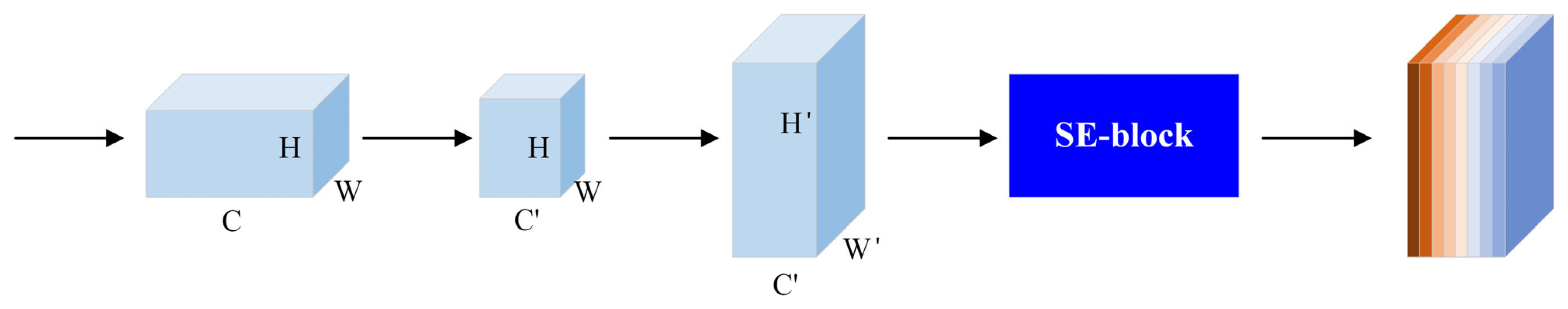
3.1. Detail-Aware Path (DAP)
Due to the lack of attention to detailed features in the MOBSN structure, it may result in the omission or incorrect detection of small targets, as well as inaccurate boundaries. This paper considered shallow features as spatial information, such as edge and structural features [
43], and proposed to fully explore the potential of convolutional neural network (CNN) shallow features through the use of the DAP. The DAP mainly consists of two stages: the first stage is spatial detail information extraction. The DAP designed in this paper has four layers, and the output resolution of each layer is 1/2, 1/4, 1/4, and 1/4 of the original resolution, respectively. The first layer used a convolution kernel of size 7 to better capture spatial features while avoiding noise interference. The second stage is feature fusion, as shown in the gray dashed box in
Figure 2, where the blue arrows represent down-sampling and the yellow arrows represent up-sampling combined with SE attention [
44]. The process can be computed as follows:
where
represents the down-sampling operation, and
represents the convolution operation of the 3rd or 4th layer of the contextual path. As shown in
Figure 3, during the up-sampling process of
, a 1 × 1 convolution and SE attention mechanism were used to reduce channel direction interference while unifying the channel numbers of the two types of features and generates the interactively fused shallow detail feature
and the contextual feature
. Through the DAP, the detail information and semantic features were adaptively aligned and interactively fused to achieve simultaneous attention to spatial details and large receptive fields and enhance spatial-temporal semantic perception.
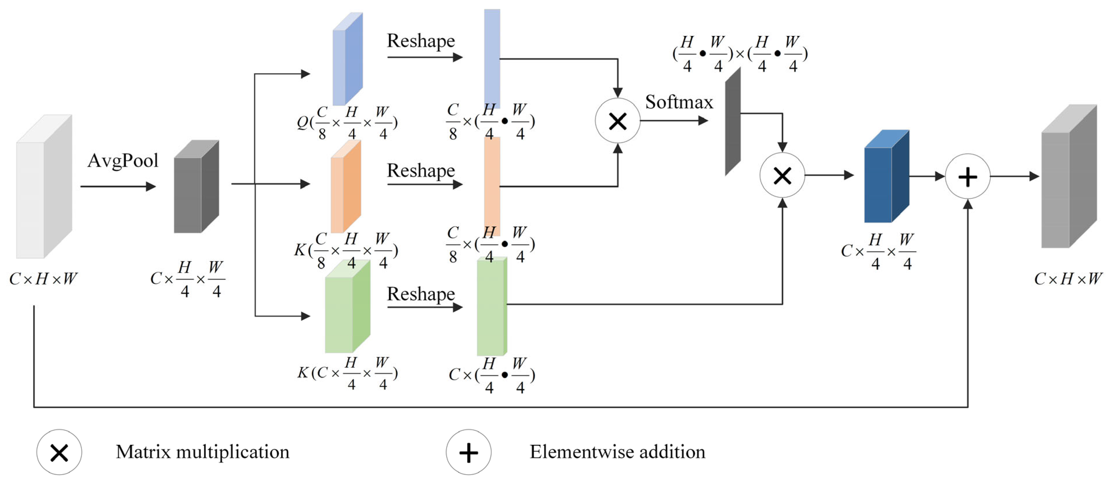
3.2. Spatial Attention Fusion Module (SAFM)
Attention mechanisms have been widely used in computer vision tasks in deep learning to help models focus on important regions in images [
45,
46]. To fully exploit the complementary characteristics of spatial details and contextual information, this study introduced the self-attention mechanism into feature fusion. The self-attention module allows each position of the output feature to attend to all positions in the input feature, fully considering the spatial dependencies between pixels. This is helpful in balancing the fusion of different types of features and generating features that are more suitable for semantic segmentation tasks.
The designed SAFM, as shown in the green dashed box in
Figure 2, is mainly divided into two stages. In the first stage, two different scales of features (contextual and detail information) were inputted into the self-attention module separately, and the weights were then adjusted using the self-attention mechanism. In order to reduce computational complexity and improve calculation speed, as shown in
Figure 4, this study applied average pooling to reduce the spatial resolution of the input features [
47]. Then, the feature
was processed through three 1 × 1 convolutions to obtain the three feature vectors
Q (queries),
K (keys), and
V (values). Attention was calculated using the vectors
K and
Q to measure the similarity between each predicted pixel and the other pixels in the image, enhancing or reducing the value of the predicted pixel. The second stage conducted was fusion. Through the self-attention mechanism, the weights of the two types of features were adjusted, and the unified spatial resolution (1/4 of the original resolution) was achieved. Then, the two types of features were concatenated and the channel number was adjusted through the convolution operation. In short, the method proposed in this article improves the feature fusion effect through the self-attention mechanism, taking into full consideration the spatial dependencies between pixels. Through adaptively adjusting the contributions of different features based on their respective attributes [
48], this method achieves the selective weighting of features to enhance spatial semantic perception, thus improving the accuracy of the semantic segmentation results obtained.
3.3. Temporal Refinement Detection Module (TRDM)
This paper drew on category attention in the field of SS [
49] to optimize the BCD subtask and designed a TRDM to achieve coarse-to-fine change detection. This module typically uses category attention to enhance the model’s sensitivity to change regions, thereby obtaining more accurate change detection results.
The change detection branch designed in this paper is shown as the brown dashed box in
Figure 2, which mainly consists of three stages. In the first stage, coarse detection was conducted. After concatenating the features from the encoder, the TRDM used a residual block composed of two 3 × 3 convolutional kernels to extract temporal features and predict the rough BCD result. In the second stage, weight adjustment based on attention was performed. Similar to the token generation in the Transformer, the input features of the coarse BCD process were multiplied by the detection results to obtain the change class center. In the original category attention mechanism, the category center is directly multiplied by the coarse segmentation result to obtain the feature after weight adjustment. This paper adopted the pixel-enhanced representation method of the OCR module [
50] and used cross-attention to fuse the convolved change class center with the input features, enhancing the representation of the temporal semantic features. In the third stage, refined change detection was conducted. Four residual blocks were used to process the weighted adjusted temporal features to obtain more accurate BCD results. The TRDM utilized the initial change detection results to guide attention and learn temporal features, suppressing false changes caused by color distortion and feature misalignment, alleviating the influence of background noise, enhancing temporal semantic perception, and improving the robustness of the model to obtain more accurate detection results.
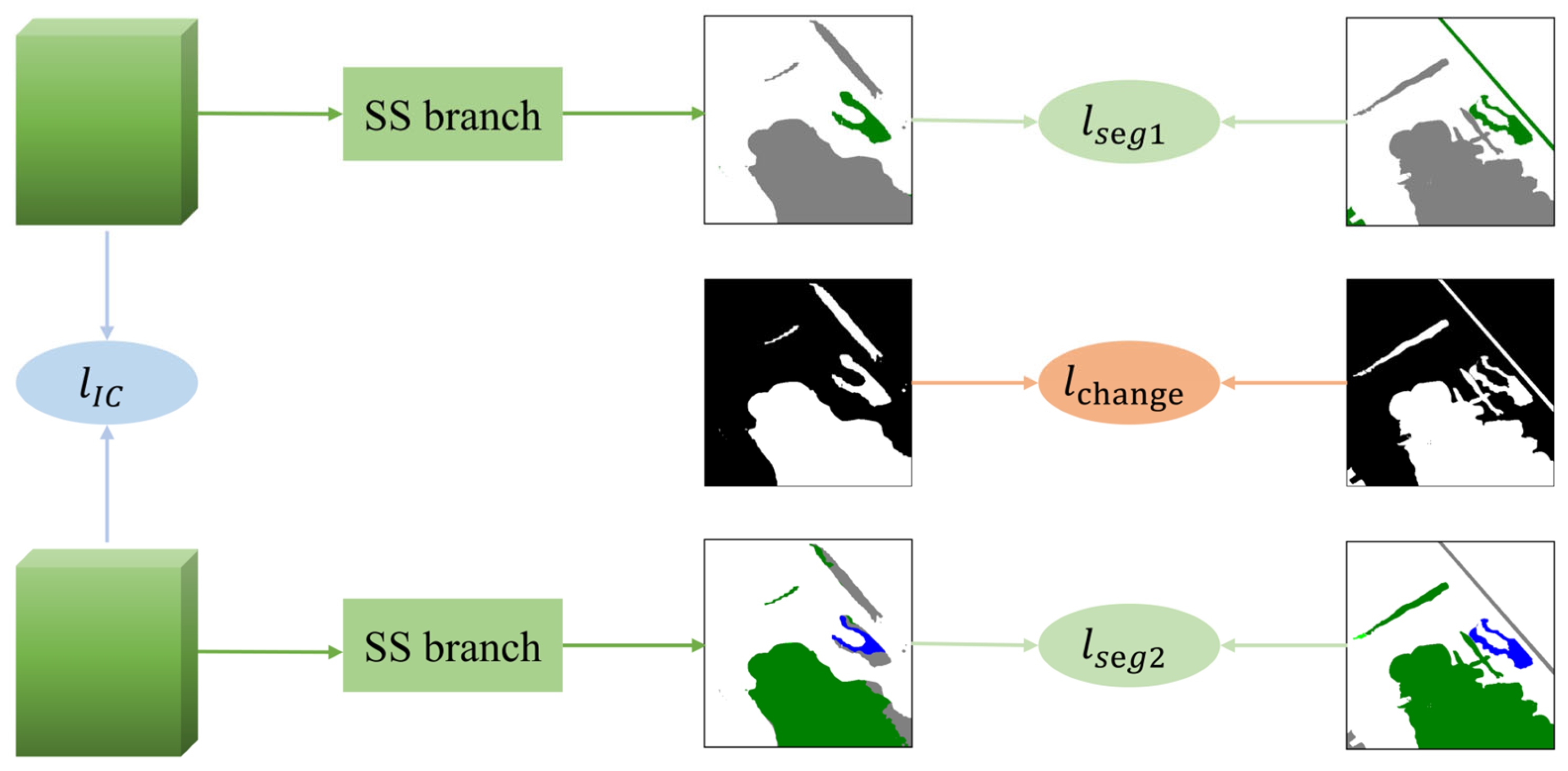
3.4. Loss Function
For the proposed STSP-Net, as shown in
Figure 5, we designed a multi-task loss function
which was as follows:
where
is the BCD loss,
is the SS loss, and
is a proposed invariant consistency loss.
The BCD loss
is the binary cross-entropy loss, which was calculated for each pixel as:
where
and
denote the ground truth (GT) label and the predicted probability of change, respectively. The GT of BCD was generated by converting non-zero label areas provided in the dataset into change regions (whereby non-zero labels were converted to “1”).
The SS loss
is the sum of losses calculated from the data of two periods, which was calculated as follows:
where
is the multi-class cross-entropy loss, which was calculated for each pixel as:
where
N is the number of semantic classes, and
and
denote the GT label and the predicted probability of the
-th class in the first period of the two periods of data, respectively, and were only included in the region with category information in the GT label.
was calculated in the same way.
In existing SCD methods, the lack of category information in the unchanged regions of the label has led most researchers to ignore the potential value of this data. To address this issue, this paper proposed to use the ICLoss
based on metric learning to unify the category information of unchanged regions in the bi-temporal images. The specific steps implemented were as follows: (1) Computerize the distance metric of the input features for the SS branch in dual-temporal images; (2) extract the distance metric values for unchanged regions; and (3) calculate the loss with the pseudo-label consisting of pixels with a value of 0. The structure of ICLoss is simple and can be applied to almost all multi-output branch SCD networks, regardless of whether the dual SS branches output the same number of categories, and it can effectively improve the detection accuracy. The above steps can be computed using the following formula:
where
represent the input features of the dual SS branches, respectively. The
function calculates the Euclidean distance between features
and
.
represents the output result of the BCD branch.
represents the Euclidean distance between
and
in the unchanged region.
can be computed using the mean squared error (MSE) loss function:
where
W and
H indicate the width and height of images, respectively.
and
represent the
result value and true value of the pixel with position
, respectively. In the ICLoss, the true label values are all zero.
The three aforementioned loss functions, , and were used to supervise the BCD branch and the SS branch, respectively, with the aim of optimizing the tasks of locating change positions and identifying change types. In addition, was used to align the semantic representations of unchanged areas, thereby mitigating the problem of pseudo-change caused by factors, such as lighting and seasons. This is beneficial for recognizing change regions and promoting the SS branch to focus more on classifying the LC categories in change regions, thereby improving the accuracy and robustness of the model.
4. Dataset and Experimental Setup
4.1. Datasets
In this study, we utilized three different datasets. To validate the effectiveness of the STSP-Net in real-world scenarios, we selected RSIs from ten provinces in China and constructed a multi-scene semantic change detection dataset called MSSCD. Additionally, to further demonstrate the superiority of the STSP-Net and enhance the credibility of comparative experiments, we also utilized two widely used datasets for SCD tasks, i.e., HRSCD [
5] and SECOND.
4.1.1. MSSCD
The MSSCD includes bi-temporal images that were randomly selected from 10 provinces in China, along with their corresponding semantic change detection labels obtained from the National Resource Survey Database. This dataset consists of 4124 pairs of images, each with a size of 512 × 512 pixels. These images were manually assembled from a variety of satellites, including the Beijing-2 Satellite (BJ-2), Gaofen-2 Satellite (GF-2), and RapidEye Satellite (RE), with spatial resolutions ranging from 0.5 m to 2 m. As shown in the third column of
Figure 6a, the dataset provides true labels for various types of changes and unchanged built-up areas between the two-phase images. We selected seven types of changes for experiments from the MSSCD, and the land cover types before the changes for each type were all non-building land, while the land cover types after the changes are shown in
Table 1. The dataset was randomly divided into the training set (70%), validation set (20%), and test set (10%). In addition, the MSSCD provides unchanged built-up areas, where the real change area should not appear.
4.1.2. SECOND
The SECOND is a dataset that was designed for SCD tasks [
14]. It includes a total of 4662 pairs of aerial images that are distributed across cities, such as Hangzhou, Chengdu, and Shanghai. Each image in the dataset has a size of 512 × 512 and contains RGB channels, with spatial resolutions ranging from 0.5 m to 3 m. As shown in
Figure 6b, in the fourth and fifth columns, the changed areas in the SECOND accounted for 19.87% of the total image, and the dataset only provided pixel-wise labels for the changed areas, including six LC (land cover) classes, which were as follows: no change, non-vegetation ground surface (n.v.g. surface for short), trees, low vegetation, water, buildings, and playgrounds. The details of each LC class are shown in
Table 2. Among the 4662 pairs of images, 2968 pairs are publicly available. Since the dataset does not have a standard partition, we randomly split it into training, validation, and test sets in a ratio of 7:1:2.
4.1.3. HRSCD
The HRSCD contains 291 aerial images pairs of 10,000 × 10,000 pixels from the BD ORTHO database, with a spatial resolution of 50 cm. As shown in
Figure 6c, the HRSCD provides two land use maps corresponding to two periods of images (the fourth and fifth columns in
Figure 6c) and the changed areas between the two periods. There are six LC categories in the land use map: artificial land, agricultural area, forest, wetland, water, and no change. The detailed information of each LC category is shown in
Table 3. Considering the expensive training cost brought with the original 10,000 × 10,000 pixel images, this paper used the zero-overlap rule grid cutting method to crop the original images into 512 × 512 pixels and focused on the changed areas, which, to some extent, alleviated the extreme class imbalance problem of the dataset. Finally, we selected 9465 pairs of images, which were randomly divided into training, validation, and testing sets in a ratio of 3:1:1.
4.2. Evaluation Metrics
In this work, we used three types of evaluation metrics to evaluate the accuracy of the total task of SCD and its two subtasks (BCD and SS). These metrics include SCD accuracy indicators: overall accuracy (
), separated Kappa (
) coefficient [
14], and
[
16]; BCD accuracy indicators: mean intersection over union (
) and
score; and the SS accuracy indicator: the
coefficient. We calculated the confusion matrix
through the prediction results and labels, where
represents the number of pixels that are classified into class
while their GT index is
(
) (the GT index corresponds to the LC category in
Table 1,
Table 2 and
Table 3). Among them, the more important metrics can be calculated using the following equations.
The
coefficient is calculated as:
is calculated as:
The
score is calculated as:
coefficient is calculated as:
Through the incorporation of the above three types of evaluation metrics, the accuracy of the SCD tasks can be comprehensively evaluated.
4.3. Experimental Settings
The experiments in this paper were run on a desktop workstation equipped with an Intel(R) Xeon(R) Gold 5222 CPU @ 3.80 GHz, a NVIDIA GeForce RTX 3090 GPU with 24 G memory. The STSP-Net network used different initial learning rates on different datasets. The initial learning rate was set to 0.01 for the MSSCD, 0.1 for the SECOND, and 0.001 for the HRSCD. Other parameters, including batch size (8), running epochs (50), and learning rate adjustment strategy, were kept consistent across all datasets. We used the stochastic gradient descent (SGD) optimizer and applied data augmentation strategies, such as normalization, random flipping, and rotation. Additionally, this study experimentally determined the optimal weight coefficients for the different loss functions in the multi-task loss, with = 1, = 0.35, and = 0.025.
4.4. Comparative Methods
To comprehensively evaluate the performance of the proposed STSP-Net, we compared it with five methods that have shown excellent performance in SCD tasks. These methods include:
The L-UNet [
51]: This method is a UNet-like network, which can simultaneously handle CD and SS using fully convolutional long short-term memory (LSTM) networks;
The HRNet [
52]: This method uses a Siamese HRNet as its backbone network to extract multi-scale semantic information from the bi-temporal images by connecting parallel convolution streams from high resolution to low resolution. Then, based on the MOBSN architecture, two segmentation branches and one detection branch are used to generate the semantic change map;
The SCDNet [
40]: This method is based on a Siamese UNet architecture, utilizing the attention mechanism and deep supervision strategy to improve its performance;
The Bi-SRNet [
16]: This method is an improvement on the MOBSN network, using two types of semantic reasoning blocks to improve single-time semantic representation and model cross-temporal semantic correlation;
The SCanNet [
52]: The SCanNet first leverages triple ‘encoder-decoder’ CNNs to learn semantic and change features, and then introduces the SCanFormer to learn ‘semantic-change’ dependencies.
5. Results and Discussion
In this section, to validate the effectiveness of our proposed improvements and the superiority of the STSP-Net, we conducted ablation experiments on the MSSCD and compared the performance of the STSP-Net with other state-of-the-art methods on three SCD datasets.
5.1. Ablation Study
In this section, we conducted ablation experiments based on the MSSCD to evaluate the performance of the STSP-Net method and explore the impact of different components on the model performance. According to the experimental results shown in
Table 4, using ResNet50 as the network backbone performs better than using ResNet34 [
16], with a higher SCD accuracy
Fscd (55.61%). Therefore, in the following experiments, we adopted the MOBSN structure with ResNet50 as the baseline method, and gradually added the proposed improvement modules to the baseline method for ablation experiments.
According to the quantitative results shown in
Table 4, adding the DAP significantly improved the performance of the MOBSN, with an increase of 1.02% in
F1 and 1.66% in Kappa. In terms of the SCD accuracy, SeK increased by 1.1% and
Fscd increased by 1.6%, indicating that the proposed DAP exhibits a positive impact on the accuracy of both sub-tasks. Building on the MOBSN with the DAP, this paper further evaluated the performance of the ICLoss, SAFM, and TDRM.
The experimental results showed that ICLoss helps to improve the consistency of LC class in unchanged regions between the bi-temporal images and highlight the change areas, thereby improving the specified indicators, such as F1 (0.61%), Kappa (1.41%), and SeK (1.25%). In addition, the SAFM can further improve these indicators, such as Kappa (0.8%) and SeK (0.44%), indicating that using the SAFM can obtain features that are more suitable for SS tasks and achieve a good balance between spatial detailed and contextual information. Finally, we evaluated the STSP-Net, which includes all the proposed modules. The experimental results revealed that although the TDRM led to a decrease in Kappa by about 0.3%, it also greatly improved the change detection and overall performance (F1: 0.58%, SeK: 0.83%, and Fscd: 0.34%, respectively). Compared with SSCD-l, the improvement of SeK and Fscd in the STSP-Net for semantic change detection accuracy were 3.61% and 4.37%, respectively. These results demonstrate that integrating all the proposed designs in the STSP-Net can effectively improve the accuracy of SCD.
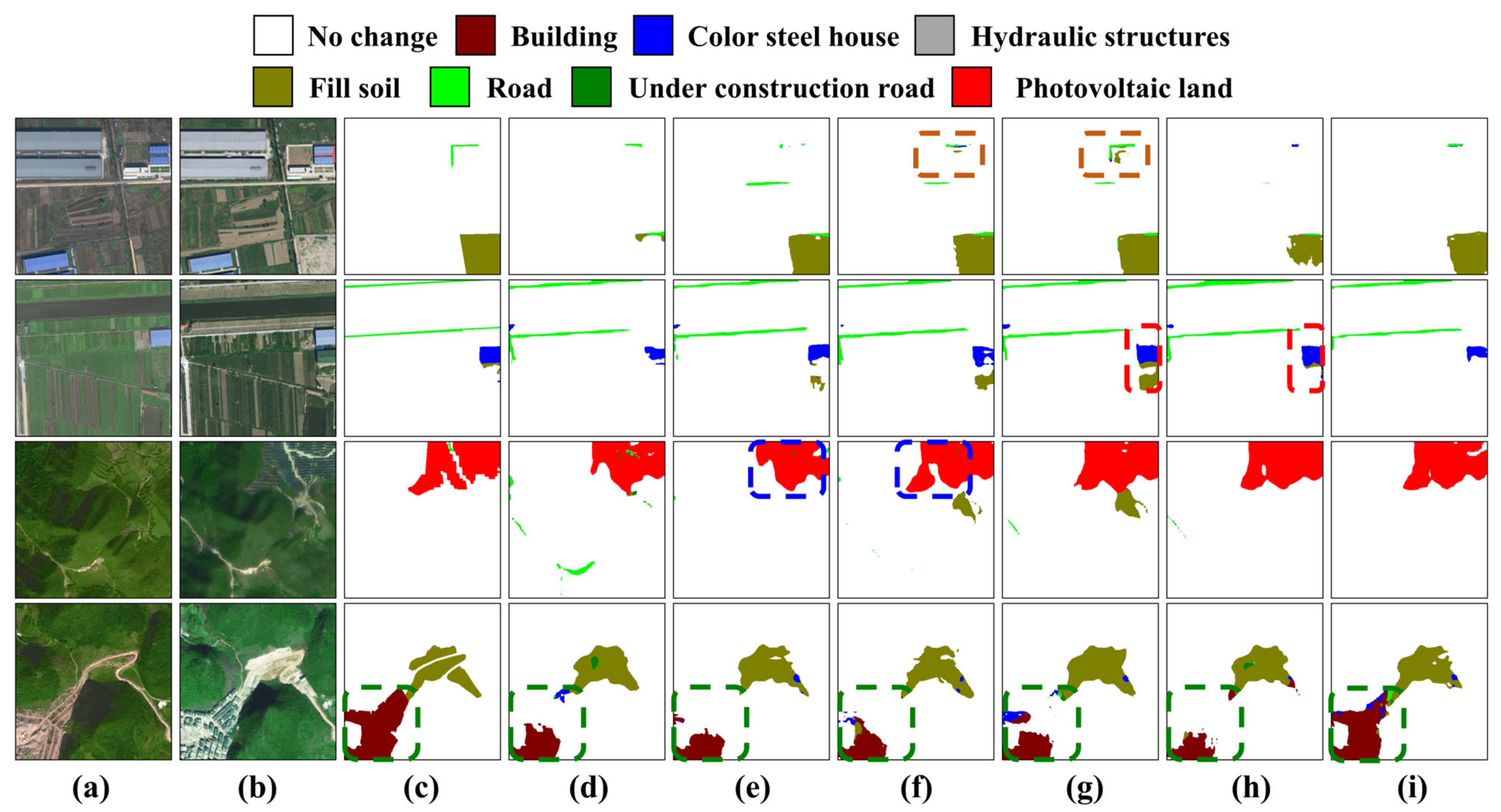
We also conducted qualitative analysis on these experimental results. In
Figure 7, we present multiple prediction results on the test set. The first three columns of
Figure 7 show the bi-temporal images and the true labels for land cover classification in the later time phase, while the last six columns show the results of the ablation experiments. Compared with the baseline, the predicted boundaries were more accurate after using the DAP to extract and fuse detailed information (such as the blue dashed boxes in
Figure 7e,f). Although there were still some false detections observed for the fill soil changes, they are difficult to be recognized even with the human eye. By integrating the ICLoss, the identified change area gradually approached the actual results (such as the brown dashed box area in
Figure 7f,g).
Then, by adding the SAFM, the predicted LC classes were improved (such as the red dashed box in
Figure 7g,h), while reducing the issue of pseudo-change. Overall, compared to the baseline method, by gradually integrating different design components, the STSP-Net identified the change areas and LC classes that are closer to the GT, as shown in the green dashed box in the fourth row of
Figure 7.
Through ablation experiments, we found that, as indicated by the improvement in quantitative metrics, extracting detailed information through the DAP and fusing it with contextual features can enhance pixel representation. Then, enhancing spatial semantic perception and temporal semantic features through the SAFM and TRDM can not only improve the recognition ability of the land cover types, but also improve the detection ability of the change areas.
5.2. Comparative Experiments
5.2.1. The MSSCD
In this section, we compared the performance of the STSP-Net with other SCD networks on the MSSCD. The quantitative results are shown in
Table 5. The STSP-Net achieved the best semantic change detection results on the MSSCD (SeK: 15.35%, F
scd: 58.97%). It is worth noting that the Bi-SRNet achieved the second-best BCD accuracy (F1: 65.88%, mIoU: 73.37%), but its semantic segmentation accuracy Kappa was significantly lower than the STSP-Net (by about 4.2%), indicating poor performance in identifying land cover categories. The HRNet achieved the second-best SS accuracy (Kappa: 78.75%).
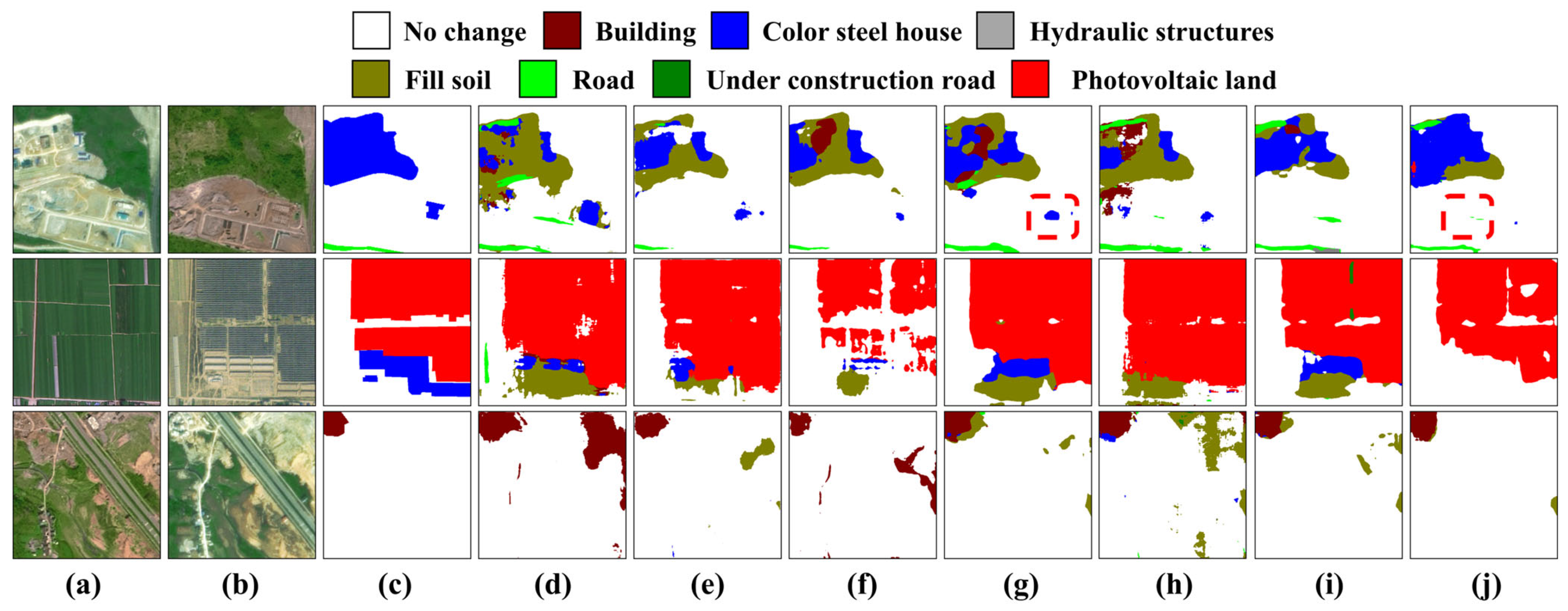
We have plotted the prediction results of the STSP-Net and other comparison methods on the MSSCD, as shown in
Figure 8. The third column of the figure only shows the true land cover categories of the post-image. From the result figures, it can be seen that the STSP-Net performs well on the test set, with fewer false labels in its prediction results compared to other comparison methods (
Figure 8, second and third rows), and the change boundaries are more accurate. However, when facing simple houses with color steel features, the change detection performance of the STSP-Net was slightly inferior to that of the Bi-SRNet (red dashed box in
Figure 8), but the land cover classification results were deemed to be much better than that method, further demonstrating the superiority of the STSP-Net in semantic change detection. It can balance the two tasks of SS and BCD well, demonstrating a better overall performance in SCD.
5.2.2. The SECOND
This section presents the comparison results of the STSP-Net and other contrastive methods on the SECOND. We used the same comparison method as for the MSSCD. The quantitative results are shown in
Table 6. The proposed STSP-Net outperformed other methods on the SECOND, with an SeK of 20.91% and
Fscd of 60.77%. Compared to the baseline method SSCD-l, this method achieved an improvement of 1.53% and 1.12% in
F1 and Kappa, respectively, indicating its effectiveness in improving the accuracy of SCD. Compared to the optimal SCanNet in the comparison method, the STSP-Net achieved an improvement of 0.91% and 1.83% in SeK and
Fscd, respectively, with a particularly notable increase of around 1.2% in Kappa for the SS subtask. It is worth noting that in the SS task, the HRNet achieved the highest Kappa, but its
F1 and SeK were both more than 3% lower than those of the STSP-Net.
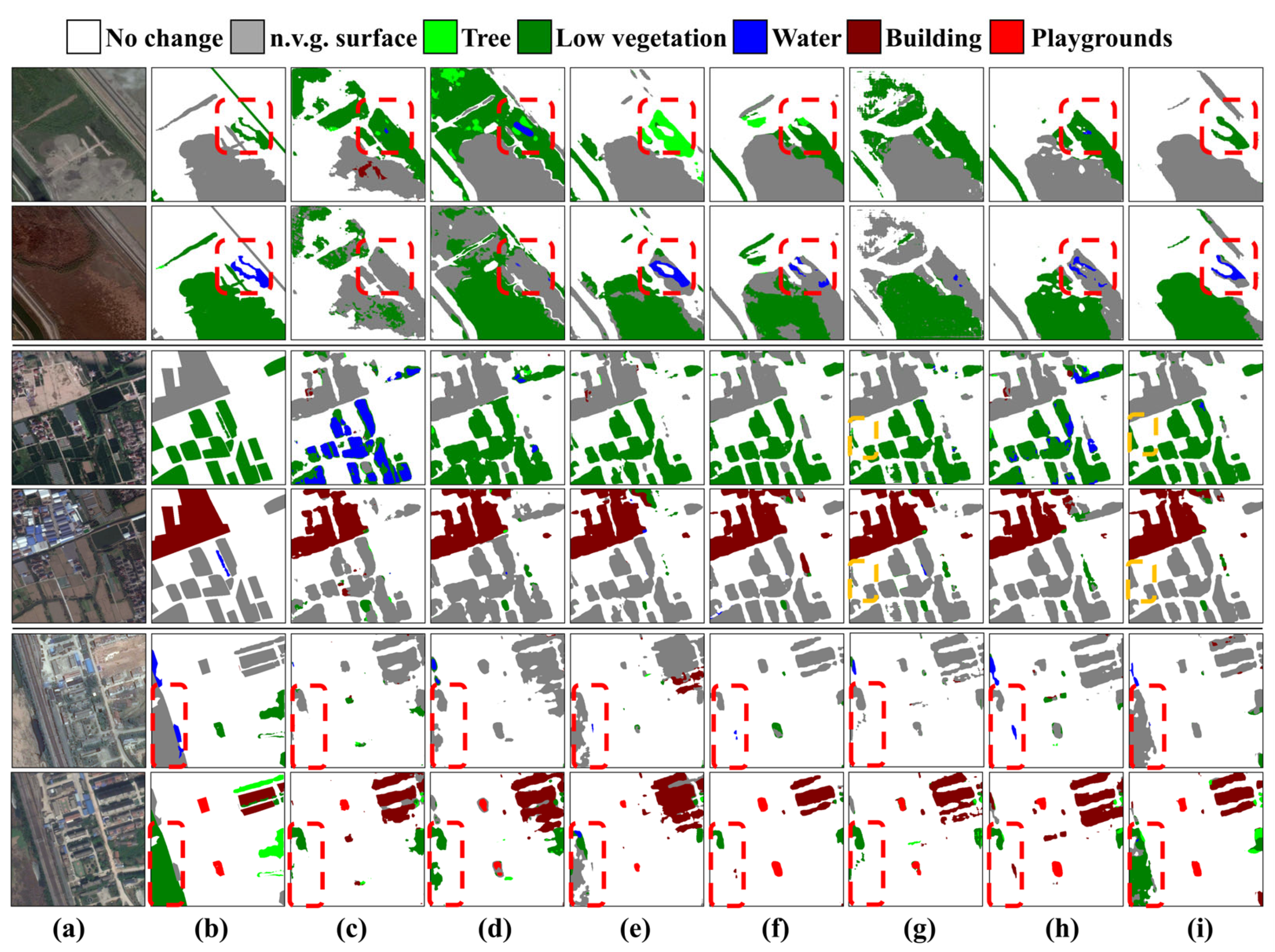
We plotted the prediction results of the STSP-Net and the comparison methods on the SECOND, as shown in
Figure 9. The first two columns of
Figure 9 show the bi-temporal images and corresponding ground truth labels of the land cover categories. As shown in
Figure 9, the STSP-Net performed well on the test set, outperforming the comparison methods in both identifying the change areas and change types (as indicated by the red dashed boxes in
Figure 9). Most changes were well recognized except for some areas. In the yellow dashed boxes in the third and fourth lines, the predictions of the STSP-Net and other methods contained several undetected change regions. However, compared with the best-performing method SCanNet in the comparison method, the missed detection regions in the STSP-Net prediction results were smaller, and the edges were closer to the real results, indicating a better overall performance.
5.2.3. The HRSCD
In this subsection, we present the test results of the STSP-Net and other comparative methods on the HRSCD, using the same comparison method as for the MSSCD. The quantitative results are shown in
Table 7. The STSP-Net achieved the best SeK (42.27%) and
Fscd (60.67%) results, surpassing all other methods in terms of BCD accuracy. Although the SS accuracy was slightly lower than that of the SCanNet, in comparison, there was a 1.45% improvement in
F1 and a 1.36% enhancement in F
scd. Compared to the comparative method Bi-SRNet, the proposed method achieved an improvement of around 1% in Kappa and 0.4% in
F1, demonstrating its effectiveness.
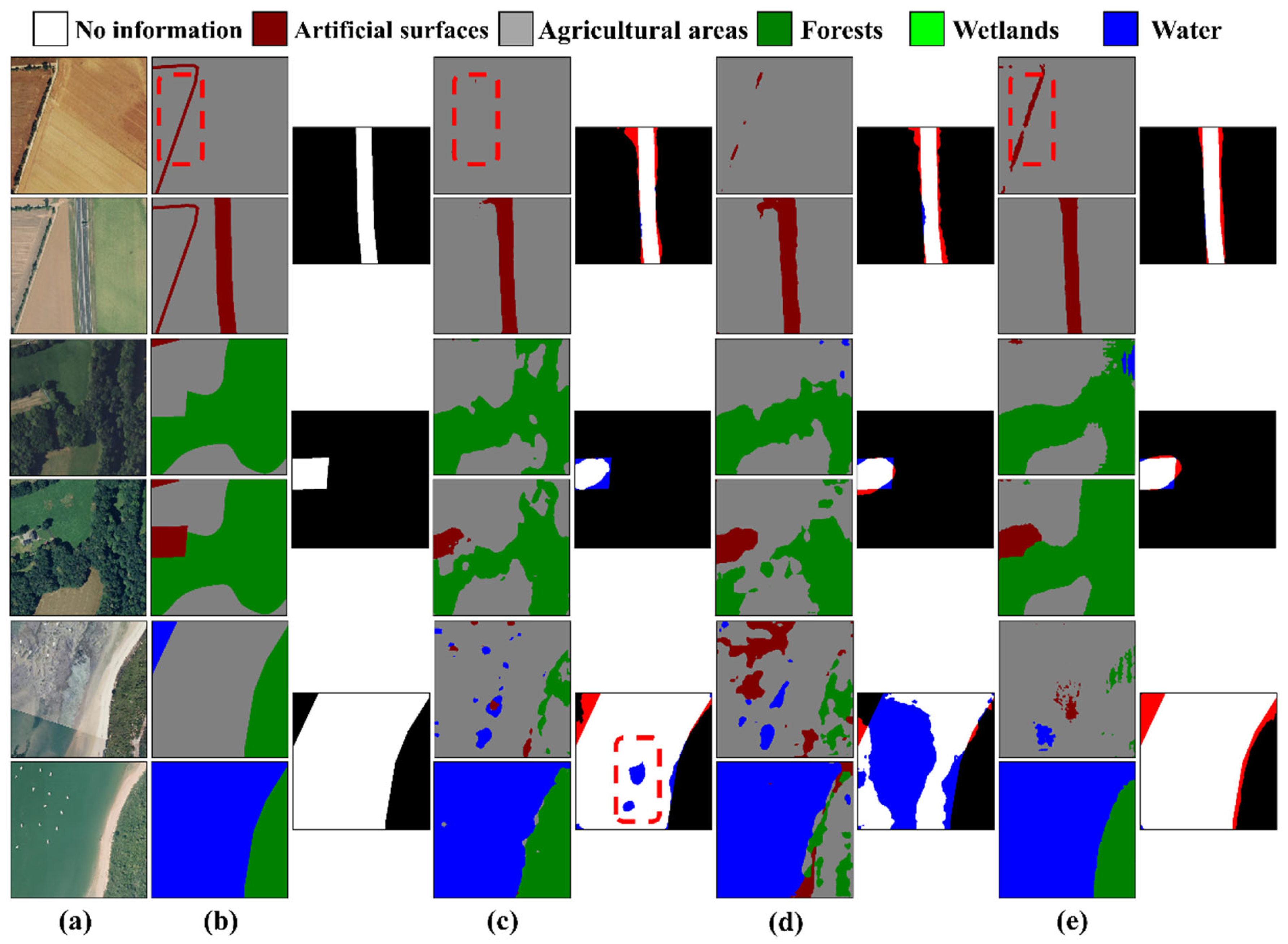
In
Figure 10, we present the predicted results of the STSP-Net and the comparative methods on the HRSCD. The first three columns of
Figure 10 show the bi-temporal images, corresponding ground truth labels of land cover, and real change labels. To better illustrate the difference between the labels and change masks, this study used the color red to indicate unchanged areas that were incorrectly identified as changed (false positives), and blue to indicate missed changed areas (false negatives). Only the predicted results of the best-performing comparative method, Bi-SRNet, are shown in
Figure 10. From the visual results, it can be observed that in the BCD subtask, the STSP-Net displayed fewer false detections and detected change areas more completely, with less occurrence of holes compared to the predicted results of the Bi-SRNet (red dashed box in the third group of
Figure 10). In the SS subtask, the Bi-SRNet may miss some thin and elongated objects, while the STSP-Net is more sensitive to details and has a higher resistance to class imbalance, alleviating such issues and achieving higher semantic segmentation accuracy (red dashed box in the first row of
Figure 10).
In summary, the original intention of the SS branch in L-UNet was to provide the semantic category as supplementary information for BCD. However, it neglected the importance of accuracy in the segmentation task, resulting in a significant imbalance between the two sub-tasks. Consequently, the SS accuracy of this method was considerably lower compared to other approaches on all three datasets. The SCDNet and HRNet use skip connections and parallel convolutional streams from high to low resolution to combine deep features and shallow details, which improves the accuracy of SCD to some extent. However, due to the limited capability of the extracted features to meet the different feature requirements of both SS and BCD, their performance remains constrained. Due to the lack of effective utilization of detailed information, both the Bi SRNet and SCanNet present a lower accuracy of SCD compared to the STSP-Net. In contrast, the STSP-Net achieved the best SCD results across all three datasets, with significant improvements in accuracy compared to the SSCD-l method. This outcome validates the efficacy of the proposed STSP-Net for SCD tasks. Furthermore, this method showcases robust generalization capabilities, reinforcing its suitability and effectiveness in addressing SCD challenges.
5.3. Discussion
5.3.1. Loss Function
To explore the performance and superiority of the ICLoss, this section compares the experimental results of the ICLoss, the semantic consistency loss (SCLoss) [
16], and the cross-entropy loss (CELoss). The underlying idea behind these three loss functions is the same, which is to ensure the consistency of class labels in unchanged regions between two temporal images. The SCLoss employs the cosine loss function to reward predictions with similar probability distributions within regions of no change while penalizing predictions within regions of change. The CELoss is based on the self-supervised learning approach introduced in the FCCDN [
42], where the segmentation results of the previous and current temporal images are used as pseudo-labels for calculating the loss of another temporal prediction.
Due to the limitations of the SCLoss and CELoss, which can only be applied when the number of classes remains consistent between the two temporal images, the comparison of the three loss functions’ performance was conducted on the SECOND. For this evaluation, the STSP-Net architecture was chosen. The experimental results are presented in
Table 8.
The aforementioned quantitative results demonstrate that, compared to the SCLoss and CELoss, SeK showed improvements of around 1.3% and 0.9%, respectively. Additionally, it achieved better accuracy in both sub-tasks, providing evidence that the proposed loss function is better suited for SCD tasks. Moreover, it is also applicable to scenarios where the number of segmentation classes varies between the two temporal images. This evidence showcases the superiority and widespread applicability of the ICLoss in the context of the semantic change detection (SCD) tasks. This highlights the versatility and effectiveness of the ICLoss in handling change detection tasks with varying class distributions across different time periods.
5.3.2. Computational Complexity
To thoroughly investigate the performance of our proposed algorithm, we conducted a detailed comparison with several baseline methods in terms of computational complexity. This comparison focused on three key metrics: parameter count (Params), floating-point operations per second (FLOPs), and inference time for every 100 images. The results of this comprehensive analysis are summarized in
Table 9.
As shown in
Table 9, the STSP-Net exhibited a lower parameter count compared to the SCDNet and HRNet, lower FLOPs than the SCanNet, and faster inference time compared to the SCDNet, HRNet, and SCanNet. These results demonstrate that our proposed method has a lower computational complexity than the more intricate algorithms used in the comparison. Additionally, as evident from the comparison results in
Section 5.2, the STSP-Net achieved a higher accuracy on all three datasets compared to the baseline algorithms. This evidence showcases that our proposed method strikes a favorable balance between algorithm complexity and accuracy, resulting in a superior overall performance. The combination of a lower computational complexity and higher accuracy validates the effectiveness of our proposed approach, highlighting its capability to achieve the highest performance while maintaining a reasonable computational load.
6. Conclusions
In this study, we proposed a novel spatial-temporal semantic perception network (STSP-Net) for high-resolution remote sensing image (RSI) semantic change detection (SCD). The proposed STSP-Net addresses the limitations of existing methods by effectively utilizing spatial detail information, enhancing spatial-temporal semantic perception, and balancing the semantic segmentation (SS) and change detection (CD) subtasks. We designed a bilateral backbone based on the Siamese network to capture spatial details and deep contextual features more effectively. Additionally, we introduced the spatial attention fusion module (SAFM) and temporal refinement detection module (TRDM) modules to enhance spatial semantic representation, improve the sensitivity of temporal features to change areas, and adaptively balance the SS and CD subtasks. Finally, the invariant consistency loss function (ICLoss) was used to constrain feature learning in unchanged areas and unify the class consistency of unchanged regions between bi-temporal RSIs.
To evaluate the performance of the proposed STSP-Net, we conducted a series of experiments on three SCD datasets. The experimental results demonstrate that the STSP-Net achieves the highest accuracy in semantic change detection.
However, we acknowledge that the proposed method still faces challenges. In the task of SCD in remote sensing, the correlation between SS and CD has not been fully utilized in the current output stage of the STSP-Net. This may lead to inconsistent results between CD and SS in the predicted outputs. Previous research do not provide a deterministic method to unify the detection results of the two subtasks. Therefore, future research will focus on increasing the information exchange between the SS branch and the CD branch, fully utilizing the causal relationship between the spatial semantic features and the temporal change representations, in order to improve the accuracy of SCD.
Author Contributions
Methodology, Y.H. and H.Z.; Validation, Y.H. and M.H.; Formal analysis, Y.H.; Investigation, X.N.; Resources, H.Z.; Data curation, R.Z.; Writing – original draft, Y.H.; Writing—review & editing, R.Z.; Visualization, D.C.; Supervision, X.N., D.C. and M.H.; Project administration, H.Z.; Funding acquisition, X.N. All authors have read and agreed to the published version of the manuscript.
Funding
This work was supported by the National Natural Science Foundation of China [grant number 42201440]; the Fundamental Research Funds for Chinese Academy of Surveying and Mapping [grant number AR2201]; and the China Postdoctoral Science Foundation [grant number 2022M712936].
Data Availability Statement
The data and the code of this study are available from the corresponding author upon request.
Conflicts of Interest
The authors declare no conflict of interest.
References
- Bovolo, F.; Bruzzone, L. The Time Variable in Data Fusion: A Change Detection Perspective. IEEE Geosci. Remote Sens. Mag. 2015, 3, 8–26. [Google Scholar] [CrossRef]
- Lv, Z.; Liu, T.; Benediktsson, J.A.; Falco, N. Land Cover Change Detection Techniques: Very-high-resolution optical images: A review. IEEE Geosci. Remote Sens. Mag. 2022, 10, 44–63. [Google Scholar] [CrossRef]
- Saha, S.; Bovolo, F.; Bruzzone, L. Unsupervised Deep Change Vector Analysis for Multiple-Change Detection in VHR Images. IEEE Trans. Geosci. Remote Sens. 2019, 57, 3677–3693. [Google Scholar] [CrossRef]
- Zhu, Q.; Guo, X.; Li, Z.; Li, D. A review of multi-class change detection for satellite remote sensing imagery. Geo-Spat. Inf. Sci. 2022, 1–15. [Google Scholar] [CrossRef]
- Caye Daudt, R.; Le Saux, B.; Boulch, A.; Gousseau, Y. Multitask learning for large-scale semantic change detection. Comput. Vis. Image Underst. 2019, 187, 102783. [Google Scholar] [CrossRef]
- Yuan, P.; Zhao, Q.; Zhao, X.; Wang, X.; Long, X.; Zheng, Y. A transformer-based Siamese network and an open optical dataset for semantic change detection of remote sensing images. Int. J. Digit. Earth 2022, 15, 1506–1525. [Google Scholar] [CrossRef]
- Zhao, M.; Zhao, Z.; Gong, S.; Liu, Y.; Yang, J.; Xiong, X.; Li, S. Spatially and Semantically Enhanced Siamese Network for Semantic Change Detection in High-Resolution Remote Sensing Images. IEEE J. Sel. Top. Appl. Earth Obs. Remote Sens. 2022, 15, 2563–2573. [Google Scholar] [CrossRef]
- El Amin, A.M.; Liu, Q.; Wang, Y. Zoom out CNNs Features for Optical Remote Sensing Change Detection. In Proceedings of the 2nd International Conference on Image, Vision and Computing (ICIVC), Chengdu, China, 2–4 June 2017; pp. 812–817. [Google Scholar]
- Tang, Y.; Qiu, J.; Zhang, Y.; Wu, D.; Cao, Y.; Zhao, K.; Zhu, L. Optimization strategies of fruit detection to overcome the challenge of unstructured background in field orchard environment: A review. Precis. Agric. 2023, 24, 1183–1219. [Google Scholar] [CrossRef]
- Wu, F.; Duan, J.; Ai, P.; Chen, Z.; Yang, Z.; Zou, X. Rachis detection and three-dimensional localization of cut off point for vision-based banana robot. Comput. Electron. Agric. 2022, 198, 107079. [Google Scholar] [CrossRef]
- Wu, F.; Yang, Z.; Mo, X.; Wu, Z.; Tang, W.; Duan, J.; Zou, X. Detection and counting of banana bunches by integrating deep learning and classic image-processing algorithms. Comput. Electron. Agric. 2023, 209, 107827. [Google Scholar] [CrossRef]
- Duan, P.; Xie, Z.; Kang, X.; Li, S. Self-supervised learning-based oil spill detection of hyperspectral images. Sci. China Technol. Sci. 2022, 65, 793–801. [Google Scholar] [CrossRef]
- Bai, T.; Wang, L.; Yin, D.; Sun, K.; Chen, Y.; Li, W.; Li, D. Deep learning for change detection in remote sensing: A review. Geo-Spat. Inf. Sci. 2022, 1–27. [Google Scholar] [CrossRef]
- Yang, K.; Xia, G.-S.; Liu, Z.; Du, B.; Yang, W.; Pelillo, M.; Zhang, L. Asymmetric Siamese Networks for Semantic Change Detection in Aerial Images. IEEE Trans. Geosci. Remote Sens. 2022, 60, 5609818. [Google Scholar] [CrossRef]
- Xia, H.; Tian, Y.; Zhang, L.; Li, S. A Deep Siamese Postclassification Fusion Network for Semantic Change Detection. IEEE Trans. Geosci. Remote Sens. 2022, 60, 5622716. [Google Scholar] [CrossRef]
- Ding, L.; Guo, H.; Liu, S.; Mou, L.; Zhang, J.; Bruzzone, L. Bi-Temporal Semantic Reasoning for the Semantic Change Detection in HR Remote Sensing Images. IEEE Trans. Geosci. Remote Sens. 2022, 60, 5620014. [Google Scholar] [CrossRef]
- Zheng, Z.; Zhong, Y.; Tian, S.; Ma, A.; Zhang, L. ChangeMask: Deep multi-task encoder-transformer-decoder architecture for semantic change detection. ISPRS J. Photogramm. Remote Sens. 2022, 183, 228–239. [Google Scholar] [CrossRef]
- Seo, D.; Kim, Y.; Eo, Y.; Park, W.; Park, H. Generation of Radiometric, Phenological Normalized Image Based on Random Forest Regression for Change Detection. Remote Sens. 2017, 9, 1163. [Google Scholar] [CrossRef]
- Holobâcă, I.-H. Glacier Mapper—A new method designed to assess change in mountain glaciers. Int. J. Remote Sens. 2013, 34, 8475–8490. [Google Scholar] [CrossRef]
- Moisan, Y.; Bernier, M.; Dubois, J.M.M. Detection of changes in a series of multitemporal ERS-1 images by principal components analysis. Int. J. Remote Sens. 1999, 20, 1149–1167. [Google Scholar] [CrossRef]
- Jin, S.M.; Sader, S.A. Comparison of time series tasseled cap wetness and the normalized difference moisture index in detecting forest disturbances. Remote Sens. Environ. 2005, 94, 364–372. [Google Scholar] [CrossRef]
- Shi, W.; Zhang, M.; Zhang, R.; Chen, S.; Zhan, Z. Change Detection Based on Artificial Intelligence: State-of-the-Art and Challenges. Remote Sens. 2020, 12, 1688. [Google Scholar] [CrossRef]
- Peng, D.; Zhang, Y.; Guan, H. End-to-End Change Detection for High Resolution Satellite Images Using Improved UNet++. Remote Sens. 2019, 11, 1382. [Google Scholar] [CrossRef]
- Li, L.; Wang, C.; Zhang, H.; Zhang, B.; Wu, F. Urban Building Change Detection in SAR Images Using Combined Differential Image and Residual U-Net Network. Remote Sens. 2019, 11, 1091. [Google Scholar] [CrossRef]
- Ghosh, A.; Subudhi, B.N.; Bruzzone, L. Integration of Gibbs Markov random field and Hopfield-type neural networks for unsupervised change detection in remotely sensed multitemporal images. IEEE Trans Image Process 2013, 22, 3087–3096. [Google Scholar] [CrossRef] [PubMed]
- Varghese, A.; Gubbi, J.; Ramaswamy, A.; Balamuralidhar, P. ChangeNet: A Deep Learning Architecture for Visual Change Detection. In Proceedings of the 15th European Conference on Computer Vision (ECCV), Munich, Germany, 8–14 September 2018; pp. 129–145. [Google Scholar]
- Daudt, R.C.; Le Saux, B.; Boulch, A. Fully Convolutional Siamese Networks for Change Detection. In Proceedings of the 25th IEEE International Conference on Image Processing (ICIP), Athens, Greece, 7–10 October 2018; pp. 4063–4067. [Google Scholar]
- Liu, M.; Shi, Q.; Marinoni, A.; He, D.; Liu, X.; Zhang, L. Super-Resolution-Based Change Detection Network with Stacked Attention Module for Images With Different Resolutions. IEEE Trans. Geosci. Remote Sens. 2022, 60, 4403718. [Google Scholar] [CrossRef]
- Zhang, R.; Zhang, H.; Ning, X.; Huang, X.; Wang, J.; Cui, W. Global-aware siamese network for change detection on remote sensing images. ISPRS J. Photogramm. Remote Sens. 2023, 199, 61–72. [Google Scholar] [CrossRef]
- Liu, Y.; Pang, C.; Zhan, Z.; Zhang, X.; Yang, X. Building Change Detection for Remote Sensing Images Using a Dual-Task Constrained Deep Siamese Convolutional Network Model. IEEE Geosci. Remote Sens. Lett. 2021, 18, 811–815. [Google Scholar] [CrossRef]
- Shen, Q.; Huang, J.; Wang, M.; Tao, S.; Yang, R.; Zhang, X. Semantic feature-constrained multitask siamese network for building change detection in high-spatial-resolution remote sensing imagery. ISPRS J. Photogramm. Remote Sens. 2022, 189, 78–94. [Google Scholar] [CrossRef]
- Chen, J.; Yuan, Z.; Peng, J.; Chen, L.; Huang, H.; Zhu, J.; Liu, Y.; Li, H. DASNet: Dual Attentive Fully Convolutional Siamese Networks for Change Detection in High-Resolution Satellite Images. IEEE J. Sel. Top. Appl. Earth Obs. Remote Sens. 2021, 14, 1194–1206. [Google Scholar] [CrossRef]
- Liu, J.; Xuan, W.; Gan, Y.; Zhan, Y.; Liu, J.; Du, B. An End-to-end Supervised Domain Adaptation Framework for Cross-Domain Change Detection. Pattern Recognit. 2022, 132, 108960. [Google Scholar] [CrossRef]
- Liu, T.; Gong, M.; Lu, D.; Zhang, Q.; Zheng, H.; Jiang, F.; Zhang, M. Building Change Detection for VHR Remote Sensing Images via Local–Global Pyramid Network and Cross-Task Transfer Learning Strategy. IEEE Trans. Geosci. Remote Sens. 2022, 60, 4704817. [Google Scholar] [CrossRef]
- Xue, J.; Xu, H.; Yang, H.; Wang, B.; Wu, P.; Choi, J.; Cai, L.; Wu, Y. Multi-Feature Enhanced Building Change Detection Based on Semantic Information Guidance. Remote Sens. 2021, 13, 4171. [Google Scholar] [CrossRef]
- Wang, X.; Du, J.; Tan, K.; Ding, J.; Liu, Z.; Pan, C.; Han, B. A high-resolution feature difference attention network for the application of building change detection. Int. J. Appl. Earth Obs. Geoinf. 2022, 112, 102950. [Google Scholar] [CrossRef]
- Wu, C.; Du, B.; Cui, X.; Zhang, L. A post-classification change detection method based on iterative slow feature analysis and Bayesian soft fusion. Remote Sens. Environ. 2017, 199, 241–255. [Google Scholar] [CrossRef]
- Yu, W.; Zhou, W.; Qian, Y.; Yan, J. A new approach for land cover classification and change analysis: Integrating backdating and an object-based method. Remote Sens. Environ. 2016, 177, 37–47. [Google Scholar] [CrossRef]
- Hao, M.; Shi, W.; Deng, K.; Zhang, H.; He, P. An Object-Based Change Detection Approach Using Uncertainty Analysis for VHR Images. J. Sens. 2016, 2016, 9078364. [Google Scholar] [CrossRef]
- Peng, D.; Bruzzone, L.; Zhang, Y.; Guan, H.; He, P. SCDNET: A novel convolutional network for semantic change detection in high resolution optical remote sensing imagery. Int. J. Appl. Earth Obs. Geoinf. 2021, 103, 102465. [Google Scholar] [CrossRef]
- Mou, L.; Bruzzone, L.; Zhu, X.X. Learning Spectral-Spatial-Temporal Features via a Recurrent Convolutional Neural Network for Change Detection in Multispectral Imagery. IEEE Trans. Geosci. Remote Sens. 2019, 57, 924–935. [Google Scholar] [CrossRef]
- Chen, P.; Zhang, B.; Hong, D.; Chen, Z.; Yang, X.; Li, B. FCCDN: Feature constraint network for VHR image change detection. ISPRS J. Photogramm. Remote Sens. 2022, 187, 101–119. [Google Scholar] [CrossRef]
- Du, H.; Zhuang, Y.; Dong, S.; Li, C.; Chen, H.; Zhao, B.; Chen, L. Bilateral Semantic Fusion Siamese Network for Change Detection from Multitemporal Optical Remote Sensing Imagery. IEEE Geosci. Remote Sens. Lett. 2022, 19, 6003405. [Google Scholar] [CrossRef]
- Hu, J.; Shen, L.; Sun, G. Squeeze-and-excitation networks. In Proceedings of the IEEE Conference on Computer Vision and Pattern Recognition, Salt Lake City, UT, USA, 18–23 June 2018; pp. 7132–7141. [Google Scholar]
- Woo, S.; Park, J.; Lee, J.-Y.; Kweon, I.S. CBAM: Convolutional Block Attention Module. In Proceedings of the 15th European Conference on Computer Vision (ECCV), Munich, Germany, 8–14 September 2018; pp. 3–19. [Google Scholar]
- Dong, X.; Lin, J.; Lu, S.; Wang, H.; Li, Y. Multiscale Spatial Attention Network for Seismic Data Denoising. IEEE Trans. Geosci. Remote Sens. 2022, 60, 5915817. [Google Scholar] [CrossRef]
- Chen, H.; Shi, Z. A Spatial-Temporal Attention-Based Method and a New Dataset for Remote Sensing Image Change Detection. Remote Sens. 2020, 12, 1662. [Google Scholar] [CrossRef]
- Zhang, F.; Chen, Y.; Li, Z.; Hong, Z.; Liu, J.; Ma, F.; Han, J.; Ding, E. ACFNet: Attentional Class Feature Network for Semantic Segmentation. In Proceedings of the IEEE/CVF International Conference on Computer Vision (ICCV), Seoul, Republic of Korea, 27 October–2 November 2019; pp. 6797–6806. [Google Scholar]
- Yuan, Y.; Chen, X.; Wang, J. Object-contextual representations for semantic segmentation. In Proceedings of the Computer Vision–ECCV 2020: 16th European Conference, Glasgow, UK, 23–28 August 2020; Proceedings, Part VI 16, 2020. pp. 173–190. [Google Scholar]
- Papadomanolaki, M.; Vakalopoulou, M.; Karantzalos, K. A Deep Multitask Learning Framework Coupling Semantic Segmentation and Fully Convolutional LSTM Networks for Urban Change Detection. IEEE Trans. Geosci. Remote Sens. 2021, 59, 7651–7668. [Google Scholar] [CrossRef]
- Wang, J.; Sun, K.; Cheng, T.; Jiang, B.; Deng, C.; Zhao, Y.; Liu, D.; Mu, Y.; Tan, M.; Wang, X.; et al. Deep High-Resolution Representation Learning for Visual Recognition. IEEE Trans Pattern Anal Mach Intell 2021, 43, 3349–3364. [Google Scholar] [CrossRef] [PubMed]
- Ding, L.; Zhang, J.; Zhang, K.; Guo, H.; Liu, B.; Bruzzone, L. Joint Spatio-Temporal Modeling for the Semantic Change Detection in Remote Sensing Images. arXiv 2021, arXiv:2212.05245. [Google Scholar]
Figure 1.
Basic framework of (a) PCCD, (b) FPSM, (c) SOBSN, (d) ISSCDN and (e) MOBSN.
Figure 1.
Basic framework of (a) PCCD, (b) FPSM, (c) SOBSN, (d) ISSCDN and (e) MOBSN.
Figure 2.
The overall structure of the STSP-Net. CCDR denotes coarse change detection results. SAFM denotes the spatial attention fusion module. TRDM denotes the temporal refinement detection module.
Figure 2.
The overall structure of the STSP-Net. CCDR denotes coarse change detection results. SAFM denotes the spatial attention fusion module. TRDM denotes the temporal refinement detection module.
Figure 3.
Combining the up-sampling process with SE attention.
Figure 3.
Combining the up-sampling process with SE attention.
Figure 4.
Structures of the basic attention module. AvgPool denotes the operation of average pooling.
Figure 4.
Structures of the basic attention module. AvgPool denotes the operation of average pooling.
Figure 5.
Calculation of multi-task loss.
Figure 5.
Calculation of multi-task loss.
Figure 6.
Example of (a) MSSCD; (b) SECOND; and (c) HRSCD.
Figure 6.
Example of (a) MSSCD; (b) SECOND; and (c) HRSCD.
Figure 7.
Performance on the MSSCD. (a) Pre-temporal images; (b) post-temporal images; (c) ground truth label of post-temporal images; (d) results of the SSCD-l method; (e) results of the MOBSN (Resnet50 serves as the network backbone); (f) results of the MOBSN with the addition of the DAP; (g) results of the MOBSN with the addition of the DAP and the ICLoss; (h) results of the MOBSN with the addition of the DAP, ICLoss, and SAFM; and (i) results of the STSP-Net.
Figure 8.
Performance on the MSSCD. (a) Pre-temporal images; (b) post-temporal images; (c) ground truth label of post-temporal images; (d) results of the L-UNet; (e) results of the SCDNet; (f) results of the HRNet; (g) results of the Bi-SRNet; (h) results of the SCanNet; (i) results of the SSCD-l method; and (j) results of the STSP-Net.
Figure 9.
Performance on the SECOND. (a) Test images; (b) ground truth label; (c) results of the L-UNet; (d) results of the SCDNet; (e) results of the HRNet; (f) results of the Bi-SRNet; (g) results of the SCanNet; (h) results of the SSCD-l method; and (i) results of the STSP-Net.
Figure 9.
Performance on the SECOND. (a) Test images; (b) ground truth label; (c) results of the L-UNet; (d) results of the SCDNet; (e) results of the HRNet; (f) results of the Bi-SRNet; (g) results of the SCanNet; (h) results of the SSCD-l method; and (i) results of the STSP-Net.
Figure 10.
Performance on the HRSCD. (a) Test images; (b) ground truth label; (c) results of the Bi-SRNet; (d) results of the SSCD-l method; and (e) results of the STSP-Net. In the change detection results, we plotted the false positives in red and the false negatives in blue.
Figure 10.
Performance on the HRSCD. (a) Test images; (b) ground truth label; (c) results of the Bi-SRNet; (d) results of the SSCD-l method; and (e) results of the STSP-Net. In the change detection results, we plotted the false positives in red and the false negatives in blue.
Table 1.
Details of each LC category in the MSSCD.
Table 1.
Details of each LC category in the MSSCD.
| GT Index | LC Category | RGB Code |
|---|
| 0 | No change | 255, 255, 255 | ![Remotesensing 15 04095 i001]() |
| 1 | Building | 128, 0, 0 |
| 2 | Color steel house | 0, 0, 255 |
| 3 | Hydraulic structures | 128, 128, 128 |
| 4 | Fill soil | 128, 128, 0 |
| 5 | Road | 0, 255, 0 |
| 6 | Under construction road | 0, 128, 0 |
| 7 | Photovoltaic land | 255, 0, 0 |
Table 2.
Details of each LC category in the SECOND.
Table 2.
Details of each LC category in the SECOND.
| GT Index | LC Category | RGB Code |
|---|
| 0 | No change | 255, 255, 255 | ![Remotesensing 15 04095 i002]() |
| 1 | Water | 0, 0, 255 |
| 2 | N.v.g. surface | 128, 128, 128 |
| 3 | Low vegetation | 0, 128, 0 |
| 4 | Tree | 0, 255, 0 |
| 5 | Buildings | 128, 0, 0 |
| 6 | Playgrounds | 255, 0, 0 |
Table 3.
Details of each LC category in the HRSCD.
Table 3.
Details of each LC category in the HRSCD.
| GT Index | LC Category | RGB Code |
|---|
| 0 | No information | 255, 255, 255 | ![Remotesensing 15 04095 i003]() |
| 1 | Artificial surfaces | 128, 0, 0 |
| 2 | Agricultural areas | 128, 128, 128 |
| 3 | Forests | 0, 128, 0 |
| 4 | Wetlands | 0, 255, 0 |
| 5 | Water | 0, 0, 255 |
Table 4.
Quantitative results of the ablation study. Values in bold font are the best.
Table 4.
Quantitative results of the ablation study. Values in bold font are the best.
| Method | OA (%) | SeK (%) | Fscd (%) | mIoU (%) | F1 (%) | Kappa (%) |
|---|
| SSCD-l | 97.65 | 11.74 | 54.60 | 73.11 | 65.15 | 75.55 |
| MOBSN (Resnet50) | 97.63 | 11.73 | 55.61 | 73.29 | 65.50 | 76.30 |
| MOBSN + DAP | 97.61 | 12.83 | 57.21 | 73.84 | 66.52 | 77.96 |
| MOBSN + DAP + ICLoss | 97.62 | 14.08 | 58.15 | 74.19 | 67.13 | 79.37 |
| MOBSN + DAP + ICLoss + SAFM | 97.69 | 14.52 | 58.63 | 74.32 | 67.30 | 80.17 |
| STSP-Net | 97.84 | 15.35 | 58.97 | 74.72 | 67.88 | 79.84 |
Table 5.
The comparison on the MSSCD. Values in bold font are the best.
Table 5.
The comparison on the MSSCD. Values in bold font are the best.
| Method | OA (%) | SeK (%) | Fscd (%) | mIoU (%) | F1 (%) | Kappa (%) |
|---|
| L-UNet | 97.07 | 2.73 | 44.83 | 70.83 | 61.24 | 56.72 |
| SCDNet | 97.57 | 10.83 | 53.42 | 72.40 | 63.91 | 75.61 |
| HRNet | 97.61 | 10.81 | 54.72 | 72.05 | 63.28 | 78.75 |
| Bi-SRNet | 97.32 | 12.51 | 55.24 | 73.37 | 65.88 | 75.66 |
| SCanNet | 96.96 | 11.70 | 52.93 | 73.11 | 65.64 | 70.70 |
| SSCD-l | 97.65 | 11.74 | 54.60 | 73.11 | 65.15 | 75.55 |
| STSP-Net | 97.84 | 15.35 | 58.97 | 74.72 | 67.88 | 79.84 |
Table 6.
The comparison on the SECOND. Values in bold font are the best.
Table 6.
The comparison on the SECOND. Values in bold font are the best.
| Method | OA (%) | SeK (%) | Fscd (%) | mIoU (%) | F1 (%) | Kappa (%) |
|---|
| L-UNet | 85.44 | 14.87 | 54.39 | 68.67 | 67.69 | 71.81 |
| SCDNet | 85.80 | 18.99 | 58.96 | 70.63 | 70.97 | 75.81 |
| HRNet | 86.74 | 17.99 | 58.32 | 69.74 | 68.81 | 78.09 |
| Bi-SRNet | 87.04 | 19.28 | 58.96 | 71.28 | 70.91 | 75.67 |
| SCanNet | 86.83 | 20.00 | 59.94 | 71.63 | 71.72 | 76.31 |
| SSCD-l | 86.72 | 18.94 | 58.91 | 70.52 | 70.52 | 76.40 |
| STSP-Net | 87.29 | 20.91 | 60.77 | 72.03 | 72.05 | 77.52 |
Table 7.
The comparison on the HRSCD. Values in bold font are the best.
Table 7.
The comparison on the HRSCD. Values in bold font are the best.
| Method | OA (%) | SeK (%) | Fscd (%) | mIoU (%) | F1 (%) | Kappa (%) |
|---|
| L-UNet | 91.63 | 39.08 | 48.98 | 66.48 | 58.09 | 70.56 |
| SCDNet | 92.99 | 38.43 | 48.32 | 63.76 | 51.39 | 73.93 |
| HRNet | 92.18 | 41.74 | 49.64 | 67.89 | 60.20 | 73.75 |
| Bi-SRNet | 92.15 | 41.49 | 54.23 | 67.70 | 60.26 | 73.28 |
| SCanNet | 91.56 | 41.78 | 52.99 | 66.85 | 59.17 | 74.60 |
| SSCD-l | 92.48 | 41.41 | 54.08 | 67.68 | 59.91 | 73.39 |
| STSP-Net | 92.16 | 42.27 | 54.35 | 67.90 | 60.62 | 74.37 |
Table 8.
The comparison of loss function on the SECOND. Values in bold font are the best.
Table 8.
The comparison of loss function on the SECOND. Values in bold font are the best.
| Loss Function | OA (%) | SeK (%) | Fscd (%) | mIoU (%) | F1 (%) | Kappa (%) |
|---|
| CELoss | 86.77 | 20.04 | 59.75 | 71.71 | 71.85 | 75.80 |
| SCLoss | 86.64 | 19.32 | 59.21 | 71.22 | 71.18 | 75.81 |
| ICLoss | 87.29 | 20.91 | 60.77 | 72.03 | 72.05 | 77.52 |
Table 9.
The comparison of computational complexity.
Table 9.
The comparison of computational complexity.
| Method | Params (Mb) | FLOPs (G) | Infer. Time (s/100 Images) |
|---|
| L-UNet | 8.99 | 93.76 | 16.55 |
| SCDNet | 35.52 | 147.31 | 20.69 |
| HRNet | 33.28 | 168.35 | 28.86 |
| Bi-SRNet | 22.29 | 190.30 | 15.28 |
| SCanNet | 26.60 | 264.94 | 20.33 |
| SSCD-l | 22.23 | 189.76 | 15.45 |
| STSP-Net | 28.35 | 244.51 | 16.55 |
| Disclaimer/Publisher’s Note: The statements, opinions and data contained in all publications are solely those of the individual author(s) and contributor(s) and not of MDPI and/or the editor(s). MDPI and/or the editor(s) disclaim responsibility for any injury to people or property resulting from any ideas, methods, instructions or products referred to in the content. |
© 2023 by the authors. Licensee MDPI, Basel, Switzerland. This article is an open access article distributed under the terms and conditions of the Creative Commons Attribution (CC BY) license (https://creativecommons.org/licenses/by/4.0/).


